The second approach is based on the crystal plasticity finite element method (CPFEM). Unlike the first approach, CPFEM is developed from the crystal plasticity constitutive model; the stress and strain fields can be calculated, and details are discussed in this section.
3.2.2. Constitutive Equations
Based on Huang [
11] and Kang et al. [
32], a crystal plasticity constitutive model considering the cyclic hardening/softening effect is developed.
The overall deformation gradient tensor can be subdivided into elastic and plastic parts:
Assuming that plastic deformation is attributed to slip only, we have
where
is the plastic part of the strain rate tensor,
stands for the slip system, and
n is the total slip systems activated in the current model.
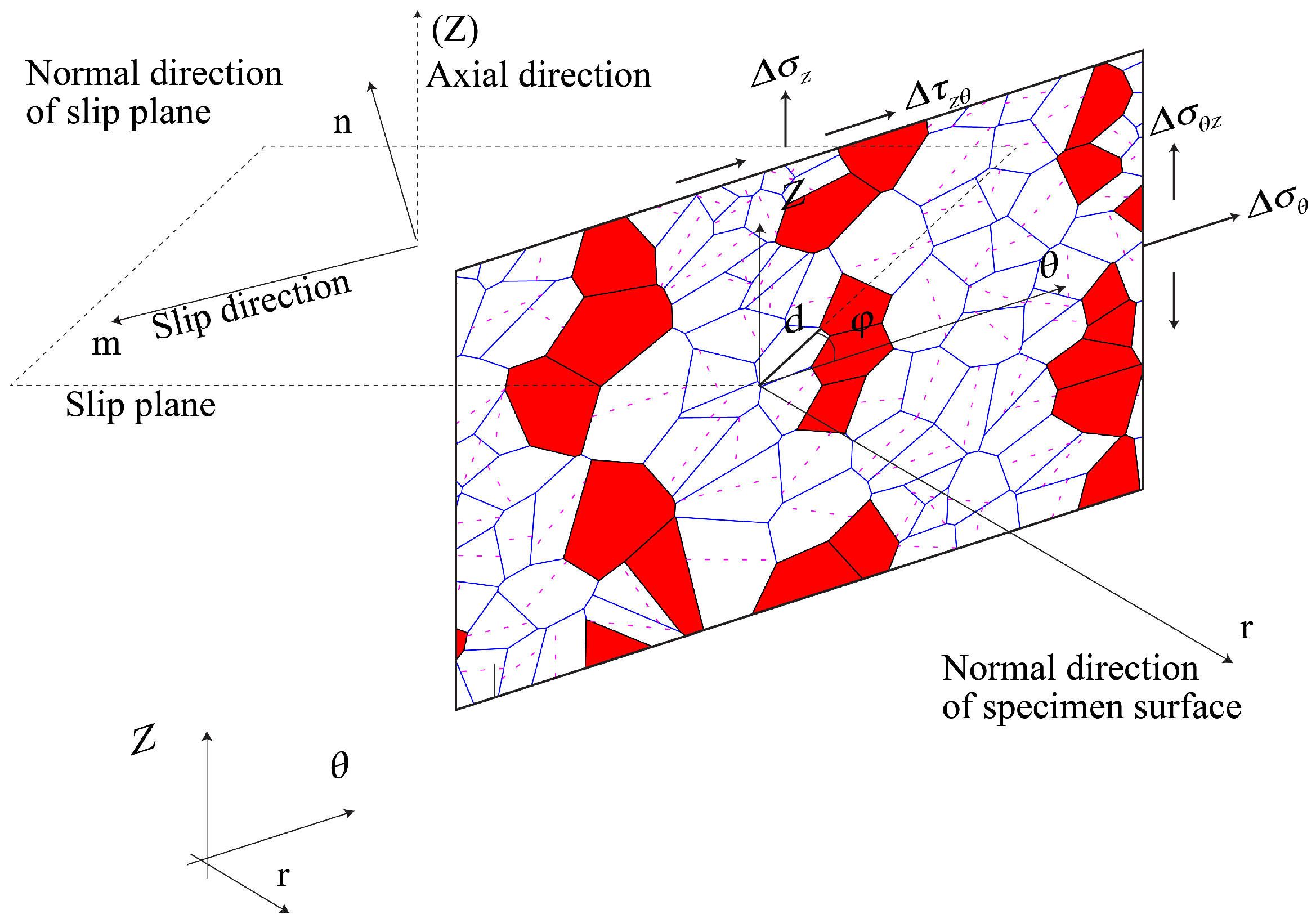
s is the slip direction vector and
m is the normal vector of the slip plane. The power-law relation proposed by Hutchinson [
33] is used in this work, modified by adding a back stress term, a slip resistance term [
32], and a cyclic hardening/softening term:
where
,
,
, and
are the cyclic hardening/softening term, resolved shear stress, back stress, and isotropic deformation resistance of slip system
, respectively,
N and
are material parameters. 〈〉 is the Macauley’s brackets:
The
term is written as:
where
S is the initial cyclic hardening/softening parameter, and
D is the cyclic parameter, which will be explained in the next section.
K and
B are parameters controlling cyclic hardening/softening, and
is the cumulative slip strain of the
th slip system. The evolution of back stress
and deformation resistance
Q is characterized by
where
is the hardening moduli, and
q is a constant representing the ratio of latent over self-hardening moduli.
A and
are direct hardening and dynamic recovery coefficients, controlling the evolution of back stress. The hardening law proposed by Bassani and Wu [
34] is adopted and simplified in this work:
where
,
, and
are the stage I stress, yield stress, and the initial hardening modulus, respectively.
The microstructure of pearlite is more complicated than that of ferrite, which makes it difficult to predict plastic deformation using the finite element method. A direct modeling of pearlite was carried out by Berisha et al. [
3] using a spectral solver developed by Roters et al. [
35]. There are some different approaches based on homogenization techniques; for example, Ashton et al. [
18] used the same constitutive model for both the pearlite and ferrite phase, with identical parameters except for the critical resolved shear stress; the simulation results showed good agreement with the experimental results. Based on the fatigue test results, no fatigue crack in the pearlite phase was observed, which made it possible to treat the pearlite phase as a homogeneous structure. Following Ashton et al. [
18], the elastic constants of the ferrite phase are set to 70% of the pearlite phase, and other parameters are same as in the pearlite phase.
In this paper, two different FIPs are adopted based on previous works [
25]. The first one is the accumulated equivalent plastic strain, which is defined as
The second FIP is defined as
where
E stands for the overall stored energy in the current structure without considering mechanical dissipation, and
is the resolved shear stress for the
slip system, as mentioned before.
3.2.3. Parameter Calibration
There are over a dozen parameters that need to be calibrated in this approach. The fatigue tests conducted in this work are under 500 °C, the elastic modulus at this temperature is 0.899 times that at room temperature (listed in
Table 2), the elastic constants at room temperature of ferrite (
,
,
) can be obtained from [
3], and the constants at 500 °C can be calculated. There are 12 parameters left to be determined; each parameter has an impact on the simulation results, which makes it difficult to calibrate all these parameters together.
Several works have been done for calibrating CPFEM parameters. For example, Bandyopadhyay et al. [
36] developed an algorithm by combining MATLAB and ABAQUS to automatically calibrate parameters. Du et al. [
20] determined some parameters by analyzing the model first, and then made some assumptions for the remaining parameters, and determined all parameters by varying them slightly to fit the experimental results. Since the CPFEM model developed in this work is applied to multiple cycles, parameter calibration needs to be done for all simulation cycles; thus, it is more convenient to make assumptions for some parameters at the beginning and then calibrate them based on the results. The material constants
N and
in Equation (
7) control the slip rate predominantly; therefore, these two parameters should be settled first. Following previous work [
37], an initial guess of
N = 20 MPa and
is made. The rest of the parameters are also set to initial values, as discussed in the following paragraph. Since
N and
only affect the flow rule of the material, after running several simulations, a stress–strain curve similar to the experimental result is obtained, and the
N and
are adjusted to 22.8 MPa and
, respectively. In the following calibration process, these two parameters will not change.
As mentioned in the Introduction, there are three sets of slip systems in ferrite, but a recent investigation showed that only
and
were activated during deformation, and the mechanical properties of these two systems were similar. Therefore, the activated slip systems are set to
and
with identical mechanical properties. In Equations (
9) and (
11), the back stress term and the cyclic term are affected by the slip rate and cumulative slip strain. To determine the parameters in both terms, a simulation without a cyclic term and back stress term (i.e.,
and
in Equation (
7)) is conducted and the average cumulative strain of 24 slip systems is measured in each increment during the whole process. Results indicate that the average cumulative strain increases
after each cycle. In this work, only the first 3000 cycles of the experiment are investigated based on the analysis of the first approach. Considering computational efficiency, it is impractical to calculate 3000 real cycles using CPFEM; hence, the cyclic parameter
D is introduced, which can scale the cumulative strain in each increment, making it possible that each cycle of CPFEM simulation represents 200 cycles of actual tests. The cyclic parameter
D in Equation (
9) should be set to 200 to scale the cumulative strain; however, the value of 200 times
after each cycle is still too small. For the convenience of the parameter calibration procedure,
D is defined as the cyclic parameter times 100; in this case,
D is set to
. The initial cyclic hardening/softening parameter
S in Equation (
9) is defined randomly but at a relatively small value to avoid a zero or negative value of
;
K is the factor controlling the value of
—in other words,
increases as
K increases.
B controls the concavity and convexity of
, which is determined to be a negative value based on the peak and valley stress evolution of the specimen shown in
Figure 11. The precise values of
K and
B are calibrated by fitting the simulation results to the experimental results.
and
in Equation (
13) control the hardening effect; previous work [
37] has shown that a simplified hardening law is effective to simulate the hardening effect. In this work,
is set equal to
; therefore, only one parameter needs to be calibrated in Equation (
13), which can be done by fitting the tensile stress–strain curve of the simulation results to the experimental results. An assumption is made that the interaction parameter
[
3,
20].
The parameters in the back stress term, i.e.,
A and
in Equation (
11), cannot be determined directly based on the slip rate. Since the back stress is not the main purpose of this work, the initial values of
A and
are set to 100 and 10, respectively. The parameter
Q in Equation (
7) represents the initial slip resistance, affecting the slip rate jointly with other parameters in Equation (
7). At this time, all parameters except
Q,
A, and
are already determined; a few simulations are carried out to calibrate the three parameters left. All calibrated parameters in this work are listed in
Table 5.
3.2.4. Simulation and Results
Firstly, a series of simulations are carried out to investigate the influence of RVE size, and three models are chosen, shown in
Figure 10. Periodic boundary conditions are assigned to each side of the RVE models and cyclic strain with 0.263% amplitude is applied, corresponding to the experimental conditions; the results are shown in
Figure 12. In this approach, stress–strain curves are calculated by multiplying the stress and strain at each integration point by the volume of the point and summing them, and then dividing this by the total volume. The integration volume is obtained from the ABAQUS field output file, and a Python script is written to perform the calculation. In a 2D model, “volume” means “area”. Based on the results, the overall stress–strain curves of the three RVE models are slightly different from each other. The stress–strain results of the models with 115 grains and 421 grains are very close, but a slight deviation is observed in the 247-grain model. As discussed in the previous section, the orientation of each grain is random. In order to investigate the influence of model size, the same random seed is assigned to the three models using NumPy [
38]. Therefore, the orientation of the same parts in the three models is identical, but the rest of the parts are different. In other words, all three models contain part of (or whole) 115 grains, and the authors can only guarantee that the orientations of 115 grains in the three models are identical. As a result, the stress–strain responses of the three models are different, but the difference is acceptable. Under the consideration of computational efficiency, the RVE model containing 115 grains is adopted. After the size of the RVE model is determined, another series of simulations are carried out to investigate the influence of mesh size. The RVE model is meshed by four different Relative Characteristic Lengths (defined in [
31]) containing 3600 elements, 8100 elements, 14,161 elements, and 22,201 elements, respectively. The simulation results are shown in
Figure 13, and the model containing 3600 elements is satisfactory. Finally, the simulation is conducted three times to evaluate the influence of grain orientation; three random orientation distributions are assigned to the model. The different orientations are achieved by assigning different random seeds to the three models (numpy.random.seed [
38]).The results are shown in
Figure 14, which indicates that the influence of orientation for the stress–strain curve is not significant.
In this paper, CPFEM simulation is conducted for 16 cycles, each representing 200 cycles in the fatigue experiment.
Table 6 lists the correspondence of cycles between experiment and simulation.
The hysteresis of the simulation and experiment is shown in
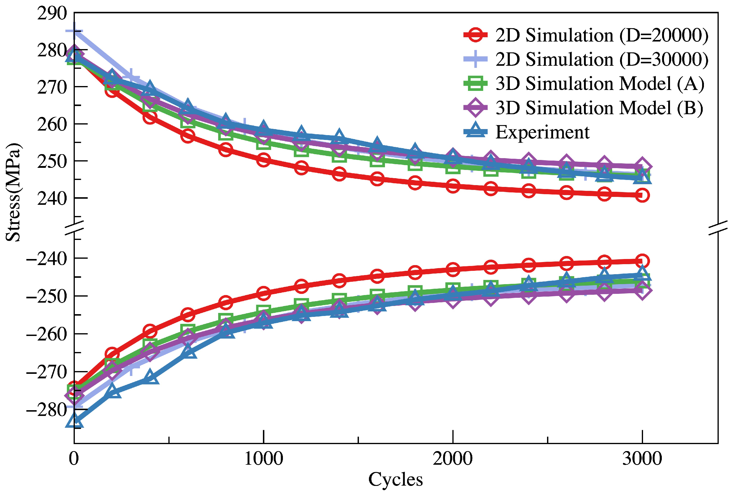
Figure 15; the simulation results of the first, 6th, 11th, and 16th cycle and the corresponding experimental results are shown here, representing the first, 1000th, 2000th, and 3000th cycle. The evolution of peak and valley stress is shown in
Figure 11. In
Figure 15, the back stress and flow stress calculated by CPFEM fit the experimental results very well, indicating that the back stress term (Equation (
11)) and the simplified hardening term (Equation (
13)) are valid. The evolution of the peak and valley stress values is also in good agreement with the experiment, which means that the constitutive model developed here is suitable for predicting the cyclic hardening/softening effect. It is noteworthy that the cyclic hardening/softening effect is introduced by reducing the strength of the crystal, explained in Equations (
7) and (
9). To demonstrate the validity of the two equations, another simulation is carried out with
D changed from 20,000 to 30,000, while other parameters remain unchanged. The results indicate that each cycle in CPFEM is able to represent 300 cycles in the experiment, as shown in
Figure 11 and
Figure 16.
Crack density and crack initiation life are determined by FIPs. The distributions of the two FIPs (
and
) are similar, as shown in
Figure 17 and
Figure 18. Areas with relatively high FIP values are more likely to be the crack initiation area. Both FIPs in the pearlite phase are set to zero because no crack is observed in it. Different crack initiation positions are observed, which are F-PGBs (marked with polygons), F-FGBs (marked with circles), and PSBs (marked with rectangles). Attempts have been made to determine the crack initiation life by setting critical values for the two FIPs, i.e., once the FIP value of an integration point reaches the critical value, it is cracked. To demonstrate the validity of the FIPs, critical values are set to
for
and
for
to ensure that the crack density is nearly 6% at 3000 cycles, as shown in
Figure 9. The evolution of crack density calculated from both FIPs is not in accordance with the experimental result, which is an expected phenomenon, because both FIPs are calculated based on the slip rate (defined in Equations (
6), (
15) and (
16)), which is obtained from Equation (
7). In Equation (
7), the slip rate is positive when the value in the brackets is greater than zero,
N and
are invariant,
increases to the same value for all grains, and
is calculated based on the Schmid factor, which changes slightly during simulation. Therefore, as long as the slip rate is positive at an integration point, the values of
and
will continue to increase, even if its stress is relatively low (less than critical resolved shear stress). This is incorrect because stress is also an important aspect of crack initiation, which means that it is difficult to determine the fatigue crack initiation life based on the previous two FIPs in this approach.
In order to predict the crack initiation life, another FIP is proposed by modifying
, explained as follows:
where
is the resolved shear stress and
is the critical resolved shear stress;
i is a constant controlling the influence of the resolved shear stress on
.
In this FIP, the accumulated equivalent plastic strain is modified. An assumption is made that the resolved shear stress and slip deformation affect fatigue crack initiation together. In this CPFEM model, according to Equation (
7), slip deformation occurs under not only high resolved shear stresses (greater than critical resolved shear stress) but also relatively low stresses (less than critical resolved shear stress); therefore, the slip deformation under low stresses should not be considered in the FIP. To this end, the effective resolved shear stress
is invoked in Equation (
19), and the effective plastic strain rate tensor is written as Equation (
18), which indicates that the contribution of the slip rate to fatigue cracking is different due to the resolved shear stress.
In the first approach, the critical resolved shear stress is set to 0.1% of the shear modulus (in Equation (
1)
= 81 MPa and
G = 81 GPa), which is a conservative assumption, because only one slip system is adopted in each grain, and the critical resolved shear stress must be set to a relatively low value in case some activated slip system is neglected (according to Equation (
1)). In this approach, the critical resolved shear stress is set to
MPa, which is 1.5 times that in the first approach. As shown in Equation (
7), the slip rate is calculated by some parameters. Theoretically, crystals will not slip if the shear stress does not reach the critical value. However, Equation (
7) cannot map this situation accurately, which means that some slip deformation under low shear stress exists, and a number of CPFEM models have the same drawback [
11]. This phenomenon may not influence the stress–strain response (as shown in this work, the results are in good agreement with experiments), but it affects the FIP values because the FIP strongly depends on slip deformation. Therefore, in order to eliminate the contribution of the “invalid slip deformation”, a larger estimation of the critical resolved shear stress is made, which is 1.5 times that in the first approach, and it gives a good result for crack density prediction. The distribution and evolution of
are shown in
Figure 19 (pearlite phase is also neglected). As with the previous two FIPs,
is also suitable for predicting crack initiation positions. To calculate the fatigue crack initiation life, the critical value of
is set to
to ensure that the crack density equals 5.9% at the end of the simulation. In order to investigate the influence of orientation on crack density, another orientation distribution is assigned to the model; the critical value of
is also determined following the same step. The crack density evolution is shown in
Figure 9 and the critical values are
and
for the two orientation distributions, respectively.
A phenomenon is observed in the magnification box of
Figure 9 wherein parts of the FIP curves are flat; the explanation is as follows. According to Equation (
19), if the stress is relatively low, the increment in the FIP is zero. As shown in
Figure 20, the corresponding stress and strain of the flat parts are relatively low, which are near
MPa to 150 MPa of stress and
to
of strain; therefore, the increment in the FIP at these parts should be zero. The threshold values of stress and strain are not symmetric, which may be caused by hardening and back stress effects.
3.2.5. 3D Geometric Models
Here, 3D geometric models are also generated and meshed by open-source software NEPER [
31]. Three models are generated with 200 grains and 300 grains (shown in
Figure 21), containing 3375 elements and 4913 elements, respectively, and the element type is C3D8 (3D 8-node brick element). As discussed in previous work [
22], the computations are rather intensive in 2D CPFEM simulations, and when moving to 3D models, the computing time is different by several orders of magnitude. For instance, the smallest 2D model in this work contains 115 grains and 3600 CPS4 elements; a simple calculation shows that if a cubic model represents the same area, it should contain approximately 1200 grains and 216000 C3D8 elements, and the computing time will increase hugely. Therefore, we use 2D models as a simplification procedure to calculate the distribution of FIPs and other details. Here, 3D models with relatively coarse meshes and fewer grains are adopted to calculate the averaged stress–strain response to demonstrate the validity of the CPFEM model. In this work, the computational time of Model (A) is 14 times that of the 115-grain 2D model.
In Equation (
7), the shear stress affects the slip rate significantly. With the element type changing from CPS4 to C3D8, the stress will also change. Therefore, the parameters in Equation (
7) need to be recalibrated. By fitting the simulation to the experimental result,
N is changed from
to 110, and all other parameters remain unchanged. The increase in
N is expected because the 2D models are simplified structures using plain stress elements to represent three-dimensional structures, and stress components
,
, and
are ignored. Since the slip rate in Equation (
7) is calculated by the shear stress (determined by Equation (
20)), the slip rate calculated by the 2D models is smaller than that obtained by the 3D models. Thus, the associated parameters need to be recalibrated.
As with 2D models, periodic boundary conditions are assigned and cyclic strain with 0.263% amplitude is applied, corresponding to the experimental conditions. Two models with different grains (Model (A) and Model (C) in
Figure 21) are calculated first to investigate the influence of RVE size, and the results are shown in
Figure 11. Comparing the experiment and 2D models, the evolution of the stress peak and valley is in good agreement. After this, four models containing 200 grains but with various orientations are calculated to demonstrate the influence of orientations. The results are similar, and two of them are shown in
Figure 22. The difference between the two orientations is acceptable, which means that the influence of orientation on the models with 200 grains is negligible. Finally, another model containing 200 grains but with different grain structures (Model (B) in
Figure 21) is calculated, as shown in
Figure 11. The structures of Model (A) and Model (B) are different, but both curves fit the experiment very well, indicating that the 3D RVE model with 200 grains is sufficient to represent the material.


