Lens Design Method Prediction of Local Optimization Algorithm by Using Deep Learning

Abstract

A design rule prediction is proposed to assist a lens design in this paper. Deep learning was applied in order to predict a lens design rule that is based on a local optimization algorithm. Three separate lens design rules related to the aperture stop and FOV variation were made for the optimization in the two-lens element optical systems whose structural parameters were created randomly. These random lens structures were optimized by using three separate lens design rules that were developed by Zemax OpticStudio API to create a big optimization dataset. All of the optimization results were collected by means of a further deep learning process to determine which optimization rule would be the better choice for lens optimization when given the lens parameters. The model developed via deep learning shows that the prediction has a 78.89% accuracy in determining an appropriate optimization rule for an assistant lens design.

1. Introduction

There are an increasing number of lens applications in everyday life, such as mobile phone cameras, endoscopes, microscopes, and so on. Different applications require different lens specifications. For example, a mobile phone camera could not be utilized as an endoscope because the object distances are different. Therefore, lens design is very important in various separate applications. Traditional lens designs are predesigned based on the Gaussian optics theory [1], which is based on the paraxial condition [2]. Under the paraxial condition, a lens is expected to be a linear system. However, a real lens with a finite aperture stop and field of view (FOV) size is often a nonlinear system; therefore, an initial lens structure must be further optimized to correspond to the specification requirements.

At present, commercial optical software provides several optimization functions for a lens design, including local [3,4] and global [5,6,7,8] optimization algorithms. The damped least square (DLS) [3,4] has now become one of the popular optimization algorithms in commercial optical software. However, the DLS algorithm is strongly related to the initial structure parameters during optimization. It is necessary to have some experience in lens design when using the DLS algorithm. Using the genetic algorithm (GA) [5,6,7,8] could search a great number of optical parameters without much more design experience. However, the GA requires a long time in optimization and cannot guarantee the best optimization result for lens design. Vasiljevic and Golobic [9] describe the advantages and the shortcomings between the DLS and GA via demonstrating the optimization of a doublet. Lens designers, in general, derive an initial lens structure from a predesign that is based on the Gaussian optics theory. According to a predesigned lens structure, local optimization algorithms are first applied to lens optimization. However, solutions of local optimization algorithms are related to not only the initial lens parameters but also the design philosophy [2]. Some design experience is necessary for lens design. Moreover, it is easy for solutions to fall into local optimization by using local optimization algorithms. After using local optimization algorithms, designers often use a global optimization algorithm instead for further optimization.

Much research has been proposed for lens optimization. Sahin [10] reviewed a classic lens design between the conventional optimization method and global optimization. Petković et al. [11] proposed a lens optimization method that is an adaptive neuro-fuzzy inference strategy. Wang et al. [12] have presented a multilayered optical design task to be a sequence generation problem. A starting point [13] is very important in lens design based on a local optimization algorithm because the initial optical parameters are strongly related to the optimization result. CÔTÉ et al. [14] have shown how to find a starting point by using deep learning method. The alternative, of which we have to be concerned in lens design, is the design philosophy. The performance of the lens design is not only related to the initial optical parameters but also to the design rules. Most lens design rules rely on the designer’s experience. It is difficult for a lens designer to determine which design rule is better for optimization, especially for given arbitrary lens parameters. Since the step of a traditional lens design is often from a small aperture stop and FOV size to find the corresponding optimization result, how to increase the increment of the aperture stop and FOV size is a key factor. We made three increment rules for a lens design. These three rules are developed by Zemax OpticStudio API and applied to a two-lens element optical system during the optimization process. The optimization results were collected to be a dataset of the deep learning process for the model construction of the design rule prediction. When the prediction model receives a set of lens parameters, it can give a better design rule for the assistant lens design.

As we know, one rule cannot be appropriate for all kinds of lens parameters in optimization. The proposal provides a design rule prediction for lens design without any conventional design experience. The optimization results regarding the three rules were analyzed by using deep learning to find which rule is the better choice for the corresponding lens parameters. The model based on deep learning shows that the prediction accuracy of the appropriate optimization rule is 78.89% when given arbitrary lens parameters. The remainder of this paper is organized as follows: Section 2 introduces a two-lens element optical system. Section 3 describes the three design rules regarding how to increase the increment of the aperture stop and FOV size. Deep learning was applied for the further analysis of the optimization data, as shown in Section 4. Section 5 concludes this paper.

2. Two-Lens Element Optical System

All optical systems with a focal point can be equivalent to two principal planes and an effective focal length (EFL) by using the Gaussian optics theory. The first step in lens design often applies a marginal ray and chief ray based on the Gaussian optics theory to determine the optical parameters, such as the EFL. These optical parameters are used to find the corresponding initial radius and thickness for a lens predesign. However, using only a single lens element cannot reach some requirements, e.g., an object and image in the same position [1]. 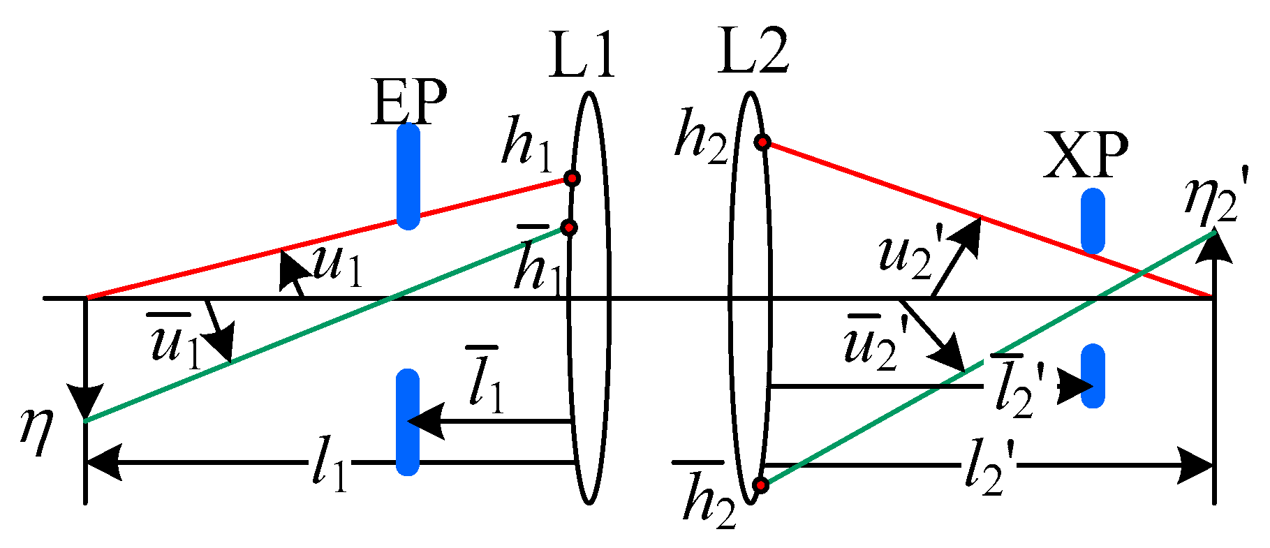A two-lens optical system (as shown in Figure 1) is used in the proposal to satisfy most requirement situations when given the specification.

There are two thin lenses (L1 and L2) shown in Figure 1. l₁ is the distance between the object and L1. The object height is η. The image is located l₂′ away from the thin lens (L2). The image height is η₂′. Figure 1 also shows the locations of the entrance pupil (EP) and the exit pupil (XP). Their positions are ${\overline{l}}_1$ and ${\overline{l\prime }}_2$ away from L1 and L2, respectively. The ray coming from the object located on the optical axis and passing the rim of the entrance pupil is the marginal ray (that is, the red ray shown in Figure 1). The marginal ray, with respect to the optical axis, forms angles ${\overline{u}}_1$ and u₂′ in the object space and image space, respectively. It also transfers to L1 and L2 at heights h₁ and h₂, respectively. There is a ray called the chief ray (the green-ray shown in Figure 1) that starts at the edge of the object and passes the center of the entrance pupil. The chief ray, with respect to the optical axis, forms angles ${\overline{u}}_1$ and ${\overline{u}}_{2\prime }$ in the object and image spaces. It transfers to L1 and L2 at heights ${\overline{h}}_1$ and ${\overline{h}}_2$. According to the paraxial condition [1,15], we can determine the following equations:

$${\overline{u}}_1=-\frac{\eta }{{\overline{l}}_1-l_1}$$

(1)

$$h_1=-u_1{l}_1$$

(2)

$${\overline{h}}_1=-{\overline{u}}_1{\overline{l}}_1$$

(3)

$$h_2=h_1\left(\frac{l_2\prime }{l_1}\right)\left(\frac{1}{M}\right)$$

(4)

$${\overline{h}}_2=\frac{H}{h_2\left(1/{\overline{l}}_2\prime -1/l_2\prime \right)}$$

(5)

where H is the optical invariant. With regard to the Gaussian optics theory, the solution of the two-lens system can be stated as follows:

$$d_{12}=\frac{{\overline{h}}_1{h}_2-h_1{\overline{h}}_2}{H}$$

(6)

$$K_1=\frac{1-{\overline{h}}_2/{\overline{h}}_1}{d_{12}}-\frac{1}{{\overline{l}}_1}$$

(7)

$$K_2=\frac{1}{{\overline{l}}_2\prime }-\frac{{\overline{h}}_1/{\overline{h}}_2-1}{d_{12}}$$

(8)

where d₁₂ is the distance between L1 and L2. K₁ and K₂ are the powers of L1 and L2, respectively. The solutions of Equations (6)–(8) are based on the paraxial condition for a two-lens system predesign. They are usually applied in order to construct an initial lens structure. Given (l₁, l₂′, ${\overline{l}}_1$, $\overline{l}{\prime }_2$, and M) randomly, as shown in

Table 1. The condition limitations for random optical parameters.

Lens Parameters	Condition Limitation
${\overline{l}}_1$	±(0~105)
${\overline{l\prime }}_2$	±(0~105)
$l_1$	±(0~105)
$l{\prime }_2$	0~102
M	±(0~102)
$u_1$	0.001 (degree)
${\overline{u}}_1$	0.001 (degree)

, the initial lens structure can be constructed according to the following:

$$K=\left(n-1\right)\left(c_1-c_2\right)$$

(9)

where K is the power of a thin lens and n is its refractive index. c₁ and c₂ indicate the curvature of the thin lens. If n is 1.5 and c₁ = c₂, then:

$$c_1=-c_2=K$$

(10)

Note that all of the parameters are created by means of exponential random distribution. However, the aperture stop and the FOV of a real lens have a finite size rather than infinitesimal. The initial lens structure has to be optimized to correspond to the real lens requirements. Common commercial optical software provides some optimization tools, such as damped least squares (DLS) and orthogonal descent. This kind of optimization algorithm that is related to the initial parameters would easily fall into local optimization. Therefore, the lens performance depends on the design philosophy.

3. Lens Design Optimization Rule

The initial lens structure is always based on the paraxial condition for a predesign, that is, a small aperture stop and FOV size. The reason is that if there are no solutions under the paraxial condition, then it must not have any solutions for real situations (i.e., a large aperture stop and FOV size). However, if a lens with a large aperture stop size and FOV is designed to meet all the specification requirements, the designed lens must have at least a solution under the paraxial condition. Since a lens design is always based on a local optimization algorithm, such as the DLS or orthogonal descent, to realize the optimization, the outcome will be related to the initial lens structure during optimization. This is the reason why a lens design is always predesigned based on the paraxial condition, with the aperture stop and FOV size gradually increasing for a real lens design. Besides the aperture stop and FOV size, the design philosophy is also related to the optimization of the image quality. We present three optimization rules for controlling the aperture stop and FOV size during the optimization process.

The fundamental aperture stop setting of the lens structure is in accordance with paraxial working F/# because the object distance is not always infinite. Moreover, we set three FOV angles, that is, 0°, 0.707$\overline{u}$₁, and $\overline{u}$₁. The merit function includes not only the default merit function of the Zemax but also the modulation transfer function (MTF) for optimization. The tangential and sagittal MTF are involved in the merit function for evaluating all FOV image qualities. As we know, the cut-off frequency of the MTF is related to the aperture stop size, that is:

$$f{\frac{1}{\lambda F/\#}}_{\max }$$

(11)

where λ is the operation wavelength. We set λ to be the d line, e.g., 0.587 μm.

The cut-off frequency, f_max, is the full frequency of the optical system. Generally, a half-frequency, or even a 1/4 frequency, is used as the standard for evaluating an optical image system. As we know, when the spatial frequency is larger, the MTF is usually lower. In order to evaluate whether the MTF of the optimized system could meet the general requirements, we required that the MTF be 0.5 f_max lps/mm > 0.3, 0.43 f_max lps/mm > 0.4 and 0.35 f_max lps/mm > 0.5 for the three FOVs. After the merit function was determined, the optimization was carried out based on the local optimization algorithm for the optical system with random optical parameters. We used three different rules to optimize the optical system and record the results of the three optimizations. Thereafter, we applied deep learning in order to analyze which rules constituted the best choice for the given random optical system parameters. Regardless of the rules, the initial values of the aperture stop and FOV were from the paraxial working F/# = 500 and ${\overline{u}}_1$ to 0.001°, respectively.

3.1. Rule 1: Progressively Increasing the Aperture Size with Constant FOV

Rule 1 is to fix the FOV size, ${\overline{u}}_1$= 1o, at the beginning with the paraxial working F/# then being set to 500. When the optimization is completed, and all the MTF requirements are met, paraxial working F/# is multiplied by m, which is initially set to 0.707 (that is, the aperture size is enlarged twice). When the MTF does not meet the requirements, the paraxial working F/# is restored to the value of the previous step, and m is set to m^0.5. The new m value is multiplied by the paraxial working F/#, and it is the setting of the new aperture. The previous steps are performed until m > 0.99 or when the paraxial working F/# is smaller than the aperture size requirement. When the paraxial working F/# is smaller than the aperture stop size requirement, the paraxial working F/# is to be set as the aperture stop size requirements, and the local optimization algorithm is performed again. Optimization rule 1 is represented in Algorithm 1 by I = paraxial working F/#. Once the paraxial working F/# meets the requirement, we gradually enlarge the FOV for optimization.

Algorithm 1. The algorithm of the aperture stop or FOV size increment.
1:	Initial increment I setting (Paraxial Working F/# = 500 or FOV = 1)
2:	Set the increment to the system and run local optimization algorithm
3:	Set value m (m = 0.707 for F/# and m = 1.414 for FOV)
4:	I = m*I
5:	While (m <= 0.99 for F/# or m >= 1.01 for FOV)
6:	Set the increment to the system and run local optimization algorithm
7:	If the optimization meet the requirements:
8:	Record the optical system date
9:	If I meet the requirement : break
10:	I = m*I
11:	else:
12:	Recover the previous optical system data
13:	I = I/m
14:	m = m0.5
15:	I = m*I

3.2. Rule 2: Progressively Increasing FOV with Constant Aperture Size

This rule is to first fix the paraxial working F/# to 500 and then to set ${\overline{u}}_1$ = 1°. After the optimization is completed and all the MTF requirements are met, ${\overline{u}}_1$ is multiplied by m. m is initially set to 1.414 (that is, double the FOV area). When the MTF does not meet the requirements, ${\overline{u}}_1$ is restored to the value of the previous step, and m is set to m^0.5. The new m value is multiplied by ${\overline{u}}_1$, which is the setting of the new FOV. The aforementioned steps are performed until m < 1.01 or when ${\overline{u}}_1$ meets the requirement. When ${\overline{u}}_1$ meets the requirement, ${\overline{u}}_1$ is to be set as the requirement, and the local optimization algorithm is to be performed again for the optical system optimization. The related algorithm is represented in Figure 2 by I = ${\overline{u}}_1$. Once the FOV meets the requirement, we gradually increase the aperture stop size for further optimization.

3.3. Rule 3: Interactively Increase the Aperture and Field Size Step by Step

According to the first two rules, the aperture and the FOV are gradually increased in an interactive sequence. When a certain termination condition is established, the optimization work is completed. We developed a program for the three optimization rules by using Zemax OpticStudio API. The lens parameters (l₁, l₂′, ${\overline{l}}_1$, $\overline{l}{\prime }_2$, and M) created randomly input three design rules we made to create a dataset for further rule prediction. Figure 2 and Figure 3 show the optimization results with the optical parameters (l₁, l₂′, ${\overline{l}}_1$, $\overline{l}{\prime }_2$, and M) = (−2.704 mm, 1.9055 mm, −1.643 mm, 105.436 mm, and −3.463) based on the rules 1 and 2, respectively. The overall length of the lens layout from rule 1 is 14.44850 mm but is 12.49450 mm for rule 2. Moreover, the thicknesses of the two-lens layout are much different. As we can observe, the lens layouts are different for rules 1 and 2. The optimization results were collected for further deep learning analysis. Moreover, the evaluation criteria were divided into four requirements based on the three different rules, as shown in

Table 2. The specification requirements.

Level	Paraxial Working F/#	$\mathbf{FOV}\left({\overline{\mathit{u}}}_1\right)$
High	<10	>10
Middle	10–14.1	7–10
Low	14.1–20	5–7
Fail	>20	<5

. Therefore, there were ten labels (all the fails from the three rules are with respect to the same label) in the deep learning analysis.

4. Lens Design Method Prediction by Deep Learning

The same design philosophy may not be the best way to optimize for all types of lenses. It is important to determine an appropriate design philosophy for the lens design when given a lens specification. However, the design philosophy is always dependent on the lens designer’s experience for optimization. It is difficult for a designer with less experience to optimize great lens performance. Using deep learning can help lens designers to determine which design philosophy is the better choice for optimization. There are two models in the deep learning process, which are supervised learning and unsupervised learning. We applied supervised learning that is based on Keras [16] to realize the deep learning process.

Deep learning requires features and labels for supervised learning. Each feature corresponds to one of the labels. The terms of the feature we employ consist of nine optical parameters, i.e., (l₁, l_2′, M, ${\overline{l}}_1$, ${\overline{l\prime }}_2$, d₁₂, K₁, K₂, and EFL) for the deep learning process. In this paper, we made three optimization rules that are based on the local optimization algorithm for a two-lens element optical system. According to the paraxial working F/# and FOV size, there are four levels assigned to each optimization rule (i.e., Table 2). However, all the fails are with respect to the same label in the deep learning process, so there are 10 labels used in the proposal.

A big data set is necessary for the deep learning process. Such a big data set is built from the features and labels. The features of the proposal are created randomly based on some of the constraints shown in Table 1. These features are inputted into three rules developed by OpticStudio API for automatic lens optimization. The result of the lens optimization from one of the features corresponds to one of the labels for a big data set construction. There are 3489 data created for this paper.

Table 3. Data set statistic.

Label	Number of Data
Label 0	2452
Label 1	55
Label 2	38
Label 3	256
Label 4	39
Label 5	62
Label 6	327
Label 7	40
Label 8	26
Label 9	99

shows the number of data for each label. Such a big data set was divided into 7:3 for the training data and testing data in the deep learning analysis to predict a optimal optical design rule for lens design.

The deep learning process consists of multiple layers for prediction. Each layer involves a weighting array. The purpose of deep learning is to find an appropriate weighting array in each layer. Figure 4 shows the deep learning flow chart for the weighting array optimization. The optical feature is first input into the multiple layers to predict a label. Such a prediction label could not be the same as the true label for the corresponding optical feature. A loss function is applied to evaluate the difference between the prediction label and the true label. The evaluation of the loss score is then used for the weighting array optimization. Figure 5 shows a neural network we used for the rule prediction in the lens design. It involves four layers between the input and output layers. Two of the four layers are drop layers to prevent the units from co-adapting too much. The feature of nine optical parameters (l₁, l_2′, M, ${\overline{l}}_1$, $\overline{l}{\prime }_2$, d₁₂, K₁, K₂, EFL) is first preprocessing by

$$X\prime =S\frac{\log \left|X\right|+1}{\max o\mathrm{rder}\left(X\right)}$$

(12)

where X is an optical parameter and S is the sign for the corresponding optical parameter. The function max order is the max power order for the same optical parameter. The pre-process data (X₁, X₂, …, X₉) are further processed to be the input layer, with 45 cells for enhancing the training process. There are 10 probabilities (that is, (Y₁, Y₂, …, Y₁₀)) in the output layer. Its sum (Y₁ + Y₂ + … + Y₁₀) is one. According to the 10 probabilities, we can determine which design rule is better in the lens design when given a specification.

The parametric rectified linear unit (PReLU) is an activation function and is used in the current paper, as shown in Figure 6. The rationale behind the adoption of the PReLU as an activation function was that since the characteristics of the lens still retained positive–negative relations after they were transformed, this function transformed the negative values while maintaining the advantages of the rectified linear unit (ReLu) because of its distribution on (−1,1). The PReLU is expressed by Equation (13):

PReLU = max(αx,x)

(13)

The PReLU can be treated as an activation function modified on the basis of the ReLU. It includes the parameter α, which processes the positive values in the same way as the ReLU and uses the weight α to process the negative values. Moreover, the weight α, which is adjusted depending on data, can be used to process the data of this study effectively.

The value parameters were expected to become nearly equivalent to the label parameters at the final phase of transforming the lens data. In this case, the model would be more capable of achieving the desirable effects. The data labels used in this study were distributed in (0,1); thus, the Softmax function was adopted as an activation function for transforming the lens data to the output layer. The distribution of Softmax is the same as that of the data labels: (0,1). The output of Softmax represents the probability of the outcomes for a predicted choice, so the function can be used to define multiple classes. The probability distributions of 10 labels were estimated, and the labels were transformed until we determined to what extent the data could be best transformed and which algorithm was the most desirable for processing the data. The probability distributions of these labels were summed up as one. The data were trained through models that varied in terms of the number of layers; the best-fit model was determined on the basis of accuracy, without taking into account the status of the input or output layer.

Table 4. Model accuracy in relation to the number of layers.

	2 Layers	3 Layers	4 Layers	5 Layers	6 Layers	7 Layers
Accuracy rate	77.55%	77.75%	78.89%	76.89%	77.27%	76.12%

compares the accuracy of the models across different layer numbers.

The experimental results showed that the neural network model, which consisted of four hidden layers, was the most accurate and that an addition of one more hidden layer to the model would have undermined its accuracy. The weight of the model was denoted by an arrow in an image. The number of neurons could be increased by adjusting the weight; the total weight of the neural network was 2962 neurons. The hidden layers contained two dropout layers, which closed the neurons randomly. The model with an accuracy of 78.89% was saved, and it was adequately accurate at predicting the characteristics of the lens.

Table 5. Details of the neural network model used in this study.

	Prediction Model for an Optical Lens
Number of layers	4 (excluding input and output layers)
Number of neurons	2962
Number of training cycles	300
Activation function	Parametric Rectified Linear Unit (PReLU) and Softmax
Optimizer	Adam
Learning rate	0.001
Loss function	Categorical crossentropy

presents the details of the model.

To prevent and eliminate overfitting, an adjusted dropout was introduced. The dropout rate in the study is set to 0.05 to suppress the overfitting problem. In Figure 7, the number of training cycles is 300, and we chose “categorical crossentropy” as our loss function. The detailed neural network parameters are listed in Table 5. Although the loss function curves exhibited minor oscillations (Figure 7), overfitting was considerably reduced after the introduction of the dropout approach, and the number of loss functions in the testing dataset for the neural network also decreased, thus improving the model’s robustness.

There are four typical criteria for deep learning classification models: accuracy, precision, recall, and the F1-score. Accuracy, in particular, is the most common and intuitive criterion; it is a ratio of the total number of predictions to the number of correct predictions. Yet, accuracy alone does not adequately reflect whether or not a model is good. A model should also be assessed with respect to its precision, recall, and F1-score. A binary confusion matrix can be used to describe the relations between classification results:

The True Positive (TP) denoted a positive true and a positive prediction; the True Negative (TN) denoted a negative true and a negative prediction, while it also referred to the number of samples correctly predicted. Conversely, the False Negative (FN) denoted a positive true and a negative prediction; the False Positive (FP) denoted a negative true and a positive prediction, while it also referred to the number of samples incorrectly predicted. The precision and recall of the model were estimated on the basis of the four outcomes shown in

Table 6. Binary confusion matrix.

	True Condition
Predicted Outcome	Total Population	Positive	Negative
	Positive	True Positive	False Positive
	Negative	False Negative	True Negative

. The F1-score of the model was derived by taking into account the precision and recall; the score ranged from 0 to 1, where 1 denoted highly satisfactory model results and 0 denoted less satisfactory model results. The precision, recall, and F1-score of the model were, respectively, estimated using the following equations:

$$\mathrm{Precision}=\frac{\mathrm{TP}}{\mathrm{TP}+\mathrm{FP}}$$

(14)

$$\mathrm{Recall}=\frac{\mathrm{TP}}{\mathrm{TP}+\mathrm{FN}}$$

(15)

$$\mathrm{F}1-\mathrm{score}=\frac{2\times \mathrm{Precision}\times \mathrm{Recall}}{\mathrm{Precision}+\mathrm{Recall}}$$

(16)

When it comes to addressing multi-class problems, accuracy, precision, and recall should all be estimated to yield their respective values. The model examined in this study was multi-class in nature, and its F1-score was calculated by using a Sklearn toolkit to perform a weighted average calculation of the precision and recall, as expressed by the following equations:

$$W_1:W_2:\dots :W_{10}=N_1:N_2:\dots :N_{10}$$

(17)

$$\mathrm{Weighted}-\mathrm{Precision}=P_1\times W_1+P_2\times W_2+\dots +P_{10}\times W_{10}$$

(18)

$$\mathrm{Weighted}-\mathrm{Recall}=R_1\times W_1+R_2\times W_2+\dots +R_{10}\times R_{10}$$

(19)

where W is the weight of all the labels and its value is the ratio of the labels; P is the accuracy of the 10 labels, and R is the recall of the 10 labels. This procedure accounted for data imbalances while yielding objective results for assessing the model. After an analysis—which used raw data corresponding to the prediction data—was conducted to assess the reliability of the model’s F1-score, the score was estimated to be as high as 0.800415, suggesting that the model was adequately reliable.

The confusion matrix, which contained 3489 data entries, was used to determine whether the model could effectively perform classification. Figure 8 shows the confusion matrix, which presents the raw data corresponding to the prediction data for the neural network.

As the confusion matrix suggested, the prediction and true values were most similar at label 0, where a preponderance of samples existed, and the prediction was more accurate. Additionally, the model showed high prediction performance at labels 3 and 6 and could analyze the outliers. The model also became confused when making predictions with these two labels, which suggested that it yielded better results if the first and second optimization algorithms were used and that both algorithms might have been comparable in optimizing the lens data.

5. Conclusions and Future Works

In this paper, a design rule prediction is presented for an assistant lens design in optimization. A two-lens element optical system is employed in the proposal because it can satisfy almost all the requirement situations that a single lens cannot implement (e.g., the object and image at the same position). The optical parameters consist of (l₁, l₂′, ${\overline{l}}_1$, $\overline{l}{\prime }_2$, and M) for the construction of the two-lens element optical system. As we know, a lens design rule cannot fit all kinds of lens structures in optimization. It is difficult to apply a single design rule for all kinds of lens structures during optimization. Moreover, the aperture stop and field of view (FOV) size are key factors in lens design. There are three design rules that are related to the aperture stop and FOV variation in lens optimization. These three design rules are developed by Zemax OpticStudio API to automatically optimize lens structures whose optical parameters (l₁, l₂′, ${\overline{l}}_1$, $\overline{l}{\prime }_2$, and M) are created randomly. As a result, the performances of the lens structures are related to the design rule, which would be classified into 10 labels for a further process of the design rule prediction. Using the deep learning method can help lens designers to determine which design philosophy is the better choice for optimization. Due to the unbalanced characteristics of the initial lens dataset, the overfitting problem becomes more serious. Therefore, overfitting was considerably reduced after the introduction of the dropout approach, and the number of loss functions in the testing dataset for the neural network also decreased. The testing results can verify the effectiveness of choosing optical design rules using our proposed deep learning model. The prediction model involves four layers between the input and output layers to obtain a prediction accuracy of 78.89%. Since the performance of lens optimization is strongly dependent on the design rule, it is possible that other design rules exist to give a better optimization than that of the three design rules we made. Only three design rules are not enough to give a better choice for lens optimization. Our future works are to make more lens design rules to fit various lens structures in optimization.