Diameter Prediction of Silicon Ingots in the Czochralski Process Based on a Hybrid Deep Learning Model

Abstract

The diameter prediction of silicon ingots in the Czochralski process is a complex problem because the process is highly nonlinear, time-varying, and time-delay. To address this problem, this paper presents a novel hybrid deep learning model, which combines the deep belief network (DBN), support vector regression (SVR), and the ant lion optimizer (ALO). Continuous restricted Boltzmann machines (CRBMs) are used in DBN for working with continuous industrial data. The feature aggregates the outputs from various DBNs through an SVR model. Additionally, the ALO algorithm is used for the parameter’s optimization of SVR. The newly developed model is verified with the actual production data and compared with the back propagation neural network (BPNN) and the SVR model. The simulation results demonstrate the availability and accuracy of the CRBM-DBN-ALO-SVR hybrid deep learning model.

1. Introduction

As a base material, silicon single crystal is used widely in fields such as microelectronics, solar cells, power electronics, and information technology. In the Czochralski process [1], which is the most extensive technique of growing silicon single crystal in industry, the diameter of silicon ingots is a critical parameter in technical requirements because it determines the stabilization of crystal growth, and the physical-chemical properties of crystals [2,3,4,5]. Nowadays, with the development of semiconductor technology, silicon single crystal should have the characteristics of low defects and large size.

Pulling speed is one key control variables of the crystal diameter. Some studies have been carried out on the influence of the pulling speed on the crystal diameter. Hurle presented a control method for the crystal diameter by the pulling speed, but this method is only suitable for small-size crystals [6]. Based on the lumped parameter model and the V/G theory for crystal growth, a technique based on a linear model was proposed to produce large-size crystals [7]. This method controls the crystal diameter and the growth rate simultaneously by adjusting the pulling speed and the heater power, but it overly depends on the setting of some parameters. The structure of a feed-forward control system is proposed, which has been utilized extensively in practice [8]. The control system comprises a tracking generator, a growth controller, a temperature controller, and an observer. Similarly, the input of a feed-forward controller depends on the experience curve and the controller’s parameters, which are obtained by repeated experiments. However, due to the complexity of the process and the restrictions on the use of sensors, it is not easy to describe the diameter prediction model by the mechanism.

Meanwhile, the artificial neural network (ANN) has strong mapping capability for nonlinear systems. When the number of hidden nodes is high enough, a neural network can approximate any continuous function in theory. Therefore, we can use a neural network to understand the dynamic characteristic between the crystal diameter and the pulling speed. In the past decade, ANN has been increasingly utilized in crystal growth [9]. Little research, especially on crystal growth of semiconductors, has been conducted [10,11,12,13,14,15,16]. So far, there have been mainly two research topics: parameter optimization, and the process control of crystal growth by ANN. Optimizing process parameters by computational fluid dynamics (CFD) is time-consuming [17]. The drawback of this method is that CFD data are obtained through simulation, which is not very accurate compared with the actual data.

NARX (Nonlinear AutoRegressive with eXogenous Inputs) is a recurrent dynamic network suitable for describing time-delay processes [18]. NARX has been successfully applied to time-series prediction. The current output of the network is related to the past outputs, the current inputs, and the past inputs. The NARX model is defined by Equation (1):

$$y(k)=f\left[y(k-1),y(k-2),\dots ,y(k-n_y),u(k-d),u(k-d-1),\dots ,u(k-d-n_u)\right]$$

(1)

where $y(k)$ is the current predicted value of output, and $f$ is some nonlinear function, such as a polynomial, sigmoid function, and so on. $n_u$ and $n_y$ stand for the exogenous determining input and output variables, respectively; $d$ is the time delay; and k is the discrete time. $n_u$ and $n_y$ can be determined by the Lipchitz quotients algorithm in the literature [19]. $d$ can be determined by using the identification method in the literature [20].

Generally, a three-layer BP neural network can approximate a NARX model [21]. However, the BP neural network has some disadvantages, such as slow convergence, ease of getting stuck at a local minimum value, and difficulty in optimizing [22]. It was not until recently that these problems were resolved by Adam and other momentum-based optimizers. However, they need a lot of labeled data. With the development of algorithms and improvements in the capability of computation and storage, deep learning theory can effectively solve the above problems. The deep learning algorithm has been successfully applied in different industrial fields, such as robot [23], autonomous driving [24], fault diagnosis [25], etc. The deep belief network (DBN) is a popular deep learning structure and is simple and easy to implement. Therefore, DBN is used to identify the model between the pulling speed and the crystal diameter in this paper.

In the existing literature, the applications of ANN in crystal growth are mainly focused on optimization problems. So, a novel optimization method, ant lion optimizer (ALO), will be described shortly.

This paper is structured as follows: In Section 2, the conventional control system for Czochralski silicon single-crystal growth is illustrated. Section 3 introduces some fundamental theories applied in this paper. In Section 4, a diameter prediction model is developed by a hybrid deep learning method. In Section 5, the simulations are performed to validate the availability of the proposed prediction model. Finally, the conclusion is summarized in Section 6.

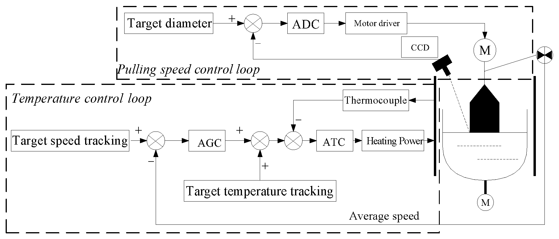
2. Description of the Object

There are many factors affecting the crystal diameter and the quality of silicon ingots in the Czochralski process, such as the pulling speed, the rotational rate of the crystal and the crucible, the position of the crystallization front, etc. Figure 1 illustrates the traditional cascade PID control structure, which is popular in practice.

The control system has two loops: the pulling speed loop and the temperature loop. In the pulling speed loop, the error between the diameter reference value and the measured value by the CCD camera is sent to the automatic diameter controller (ADC), which adjusts the pulling speed. In the temperature loop, an automatic temperature controller (ATC) regulates the thermal field temperature to compensate for thermal disturbances, such as the latent heat of crystallization, the thermal convection, and the thermal radiation. Here, the thermal field temperature refers to the temperature of an appropriate spot on the furnace wall, measured by the temperature sensor, such as an infrared sensor or a thermocouple. Since the pulling speed will directly affect the properties of the crystal, it is required that the pulling speed should track the predetermined reference trajectory tightly. For this purpose, the automatic growth controller (AGC) is designed to cascade with ATC. The AGC compares the actual pulling speed with the reference value to provide the ATC thermal field temperature that is required.

The frequent change in the pulling speed will cause some defects in the crystal. In this control structure, it is ensured that the system can respond quickly to the perturbations of the crystal diameter. The model between the pulling speed and the crystal diameter is characterized by the time delay and nonlinearity, which are challenging to deal with. So, researching the model between the pulling speed and the crystal diameter is of great importance.

3. Research Methodology

3.1. CRBM-DBN

Since Hinton et al. presented a new training algorithm for deep neural networks, the deep belief network (DBN) has been extensively used [26]. The DBN is stacked by a group of restricted Boltzmann machines (RBMs), which can understand the more complex relationship between visible and hidden units [27]. In addition, the combination of the unsupervised DBN and the supervised regression method forms a semi-supervised framework, which has better representation ability [28].

Figure 2a is the structure diagram of an RBM, which has two layers: an input layer containing visible units $v=\left\{v_1, v_2,\dots ,v_i\right\}$ and a hidden layer containing hidden units $h=\left\{h_1, h_2,\dots ,h_j\right\}$. An energy function is given by

$$E\left(v, h\right)=-{\displaystyle \sum _{i=1}^V{\displaystyle \sum _{j=1}^H{w}_{ij}{v}_i{h}_j-{\displaystyle \sum _{i=1}^V{a}_i{v}_i}}}-{\displaystyle \sum _{j=1}^H{b}_j{h}_j}$$

(2)

where $v_i$ and $h_j$ denote the states of visible unit $i$ and hidden unit $j$, $w_{ij}$ is the weight between them, and $a_i$ and $b_j$ are their biases.

A typical three-hidden-layer DBN model is shown in Figure 2b. The training process of DBN is realized in two steps: the first is pre-training, and the second is fine-tuning [29]. The contrast divergence (CD) algorithm is used for adjusting the weight parameters, and the standard back propagation algorithm is used for fine-tuning the whole DBN.

Generally, in the typical DBN structure, the logistic regression or Softmax regression is widely used as the last layer of the network, so the DBN is more suitable for solving classification problems [30,31,32]. However, the DBN is rarely applied to regression problems. Because the original units of the RBM are binary and discrete, it is impossible to model continuous values [33]. For analog data, Chen proposed a continuous RBM (CRBM) [34]. By replacing RBM with the CRBM, the traditional classification of the DBN is improved and the CRBM-DBN for regression is developed. In CRBM, binary units in RBM are replaced by continuous stochastic units, and the learning rule is “Minimizing Contrastive Divergence” (MCD) [35]. The continuous stochastic unit is as follows:

$$s_j={\varphi }_j\left({\displaystyle \sum _i{w}_{ij}{s}_i}+\sigma N_j\left(0,1\right)\right)$$

(3)

with ${\phi }_j\left(x_j\right)={\theta }_L+\frac{\left({\theta }_H-{\theta }_L\right)}{1+e^{\left(-{\alpha }_j{x}_j\right)}}$.

Where $s_i$ and $s_j$ denote the states of the units $i$, $j$, $N_j\left(0,1\right)$ represents a unit Gaussian, and $\sigma$ is a constant. ${\phi }_j\left(x\right)$ is a sigmoid function, ${\theta }_L$ and ${\theta }_H$ are the lower and upper asymptotes, and $\alpha$ determines the slope.

The CRBM-DBN removes the Logistic or Softmax layer and uses the mean square error of the predictors to calculate the fine-tuning step. Moreover, the learning steps are the same as those of DBN. A three-hidden-layer CRBM-DBN is shown in Figure 3.

3.2. Support Vector Regression

The support vector machine (SVM) [36] is a machine learning method based on statistical learning theory. It is used to solve practical problems, such as a small sample, the local minimum, etc. SVM can accomplish the classification task of nonlinear data by using the kernel functions, which map the original space onto a higher dimensional feature space so that a hyperplane is obtained for separating the data [37]. Additionally, SVM has extended to nonlinear regression problems and is known as a support vector regression (SVR) [38,39].

Suppose a training set, ${\left\{x_i,y_i\right\}}_{i=1,\cdots ,l}$, where $x_i\in R^n$ is the input and $y_i\in R^{n_h}$ is the corresponding output. The regression function is given

$$y(x)=w^T\varphi (x)+b$$

(4)

where $w$ is the weight vector, $b$ is the bias, and $\varphi \left(\cdot \right):R^n\to R^{n_h}$ is the nonlinear mapping function. The optimal parameters, $w$ and $b$, can be determined by solving the following optimization problem [40]:

$$\begin{gathered} \min J(w,\xi )=\frac{1}{2}{w}^{T}w+C\frac{1}{2}{\displaystyle \sum _{i=1}^l{\xi }_i{}^2} \\ \mathrm{s}.\mathrm{t}. y_i=w^T\varphi (x_i)+b+{\xi }_i, i=1,\cdots ,l \end{gathered}$$

(5)

where $C$ is a penalty factor and ${\xi }_i$ is the slack variables.

Constructing the Lagrange function as

$$\begin{array}{ll}L(w,b,\xi ,\alpha )& =J(w,\xi )\\ & -{\displaystyle \sum _{i=1}^l{\alpha }_i(w^T\varphi (x_i)+b+{\xi }_i-y_i)}\end{array}$$

(6)

where ${\alpha }_i$ are Lagrange multipliers. Then first-order KKT conditions are

$$\left\{\begin{array}{l}\frac{\partial L}{\partial w}=0\to w={\displaystyle \sum _{i=1}^l{\alpha }_i\varphi (x_i)}\hfill \\ \frac{\partial L}{\partial b}=0\to {\displaystyle \sum _{i=1}^l{\alpha }_i}=0\hfill \\ \frac{\partial L}{\partial \xi }=0\to {\alpha }_i=C{\xi }_i\hfill \\ \frac{\partial L}{\partial \alpha }=0\to w^T\varphi (x_i)+b-y_i+{\xi }_i=0\hfill \end{array}\right.$$

(7)

Furthermore, Equation (7) is equivalent to Equation (8).

$$\left[\begin{array}{cc}0& 1^T\\ 1& K(x_i,x_j)+C^{-1}I\end{array}\right] \left[\begin{array}{c}b\\ \alpha \end{array}\right]=\left[\begin{array}{c}0\\ y\end{array}\right]$$

(8)

where $y={[y_1; \cdots ;y_l]}^T$, $1={[1;\cdots ;1]}^T$, $\alpha ={[{\alpha }_1;\cdots ;{\alpha }_l]}^T$, $K(x_i,x_j)={\varphi }^T\left(x_i\right)\cdot \varphi \left(x_j\right) \left(i,j=1,2,\cdots ,l\right)$ is the kernel function.

Therefore, the regression function in Equation (4) is converted into a more explicit formula.

$$y(x)={\displaystyle \sum _{i=1}^m{\alpha }_{i}K(x_i,x_j)+b}$$

(9)

Because the radial basis function (RBF) has better properties under general smoothness conditions, it is selected as the kernel function in this work.

$$K(x_i,x_j)=\exp \left(-\gamma {‖x_i-x_j‖}^2\right)$$

(10)

where $\gamma >0$ is the width of the kernel function.

It is essential to set appropriate parameters, which will affect the learning and generalization capabilities of the SVR. The SVR has two parameters [41], i.e., C and γ, which can be set up through an optimization algorithm.

In this work, these parameters are optimized by a novel optimization algorithm, which is outlined below.

3.3. Ant Lion Optimizer (ALO)

ALO is a kind of swarm intelligent optimization algorithm, which is inspired by the hunting behavior of antlions [42]. The antlion is an insect of the Myrmeleontid family. In the larval phase, they mainly catch and feed on ants. The antlion digs a cone-shaped trap and waits at the bottom of the trap for the ant to fall in. When the ant is in the trap, the antlion throws sand at the ant to prevent escape. After the feeding is finished, the antlion rebuilds the trap for the next hunt. Figure 4 shows the predation behavior of the antlion.

In the ALO algorithm, ants walk in the solution space as search agents, and antlions become fitter by hunting. According to the interaction between antlions and ants in this process, the main steps are modeled mathematically as follows.

(1)

Random Walk of Ants

According to Equation (11), ants walk randomly and search the solution space.

$$\begin{array}{ll}X=& [0,cumsum(2r(1)-1),cumsum(2r(2)-1),\cdots ,cumsum(2r(t)-1)\\ & \cdots ,cumsum(2r(T)-1)]\end{array}$$

(11)

where $X$ is the vector of walk position; $cumsum$ is the cumulative sum; $T$ is the maximum number of iterations; $t$ is the current number of iterations; and $r\left(t\right)$ is the stochastic function calculated by

$$r\left(t\right)=\left\{\begin{array}{c}1 if rand>0.5\\ 0 otherwise \end{array}\right.$$

(12)

where $rand$ function returns a random number between 0 and 1.

To keep the walks within the search space, they are normalized by the min-max normalization method.

$$Z_i^t=\frac{\left(X_i^t-a_i\right)\times \left(d_i^t-c_i^t\right)}{\left(b_i-a_i\right)}+c_i^t$$

(13)

where $Z_i^t$ normalized walk position of $i$th variable at $t$th iteration. $a_i$ and $b_i$ denote the minimum and maximum of $i$th variable, and $c_i^t$ and $d_i^t$ denote the minimum and maximum of $i$th variable at $t$th iteration.

(2)

Entrapping ants

Since the walk of the ant is influent by the antlion’s trap, it can be described by Equation (14).

$$\left\{\begin{array}{c}{c}_i^t=Antlio{n}_j^t+c^t\\ d_i^t=Antlio{n}_j^t+d^t\end{array}\right.$$

(14)

where $c^t$ and $d^t$ are minimum and maximum of all variables at $t$th iteration, $c_i^t$ and $d_i^t$ are minimum and maximum of all variables for $i$th ant, and $Antlio{n}_j^t$ is the position of $j$th antlion at $t$th iteration.

(3)

Building Trap

Supposing an ant is trapped by only one selected antlion, the roulette wheel operator is used to select an antlion. This mechanism gives a fitter antlion more opportunities to hunt ants.

(4)

The ant gliding to the antlion

Once an ant falls into the trap, the antlion will shoot sand to slide down the ant, and the radius of the ant’s walk will shrink. This behavior is modeled by Equation (15).

$$\left\{\begin{array}{c}{c}^t=c^t/R\\ d^t=d^t/R\end{array}\right.$$

(15)

where $R={10}^{p}t/T$, $p$ is

$$p=\left\{\begin{array}{c}2 if t>0.1T\\ 3 if t>0.5T\\ 4 if t>0.75T\\ 5 if t>0.9T\\ 6 if t>0.95T\end{array}\right.$$

(5)

Capturing prey and rebuilding the trap

Finally, the ant reaches the bottom of the trap and is eaten by the antlion. This means that the ant’s fitness is better than the antlion’s fitness. The antlion must update its position. The process is expressed as follows:

$$Antlio{n}_j^t=An{t}_i^t if f(An{t}_i^t)>f(Antlio{n}_j^t)$$

(16)

where $f$ is the fitness function.

(6)

Elitism

The best antlion is regarded as the elite, which is saved in iteration. Then, the walk of all ants is affected by the elite and the antlion selected by roulette wheel simultaneously,

$$An{t}_i^t=\frac{R_A^t+R_E^t}{2}$$

(17)

where $R_A^t$ and $R_E^t$ denote the random walks around the selected antlion and the elite at $t$th iteration.

Zhao X. et al. presented an improved ALO algorithm of continuous radius contraction and dynamic random search [43,44], which has better convergence speed and optimization accuracy. Additionally, it is adopted for the parameter optimization of SVR.

4. Diameter Prediction Model Based on CRBM-DBN-ALO-SVR

For regression, when the epoch of back propagation training changes, the results differ. Therefore, we can integrate all of the outputs generated by the DBNs with a different number of epochs. By analyzing each output and predicted output, the corresponding weight is assigned to each output to calculate the overall predicted output. In this study, we propose a hybrid deep learning model based on the CRBM-DBN-ALO-SVR for diameter prediction. All of the outputs of the DBNs are obtained using a different number of epochs, and the final prediction is obtained as the output of an SVR whose inputs are the outputs of the DBNs. ALO is used to optimize the SVR parameters. The proposed model is illustrated in Figure 5.

The specific procedures are as follows:

(1) Initializing the network parameters (weight vector $W$ and the offset $a,b$, learning rate, etc.); training the CRBM using the contrast divergence method and adjusting the weight vector and the offset; and training the DBN network by using the layer-by-layer CRBM.

(2) Using input data X to fine-tune the DBN’s parameters by using the gradient descent method.

(3) Setting the back propagation epoch from 100 to 2000 and the step size to 100, and obtaining 20 prediction outputs, from Y₁ to Y₂₀.

(4) Training an SVR with the output data matrix Y and 20 prediction outputs from the DBNs. The parameters of the SVR are optimized by an improved ALO algorithm.

(5) The output of the SVR is considered the final predicted value.

The flowchart of this hybrid deep learning method is shown in Figure 6.

5. Results

In this section, some simulations are made to test the proposed model. The software and hardware of the computational platform are shown in

Table 1. Instructions for the computational platform.

Software and Hardware	Configuration
Operation System	Windows 10 Professional
CPU	i5-4590, 3.7 GHz
RAM	8 GB
Matlab	R2016b

.

5.1. Data Source and Evaluation Indices

The simulations make use of the measured data from a TDR-150 Czochralski single-crystal growth furnace, which is represented in Figure 7.

The main production parameters are as follows: the feeding amount is 90 kg, the furnace pressure is 20 Torr, the argon flow rate is 100 L/min, the rotational rate of the crucible is 9.5 rpm, and the rotational rate of the crystal is 7 rpm. The set value of the crystal diameter is 208 mm, and the data sampling time is 2 s. Data on the crystal diameter and the pulling speed are shown in Figure 8, which has been processed by moving-average filtering.

Because the magnitude of the crystal diameter is different from that of the pulling speed, the data are firstly normalized to the range [0, 1]. In light of the modeling requirements, the data are divided into a training data and a testing data.

To better evaluate the proposed prediction model, two indices are adopted in this paper: the mean absolute error (MAE) and the root mean square error (RMSE).

$$MAE=\frac{1}{N}{\displaystyle \sum _{t=1}^N\left|e_t\right|}$$

(18)

$$RMSE=\frac{1}{N}\sqrt{{\displaystyle \sum _{t=1}^N{e}_t^2}}$$

(19)

where $e_t={\widehat{y}}_t-y_t$, $t$ is the sampling time, $N$ is sample size, $y_t$ is a measured value, and ${\widehat{y}}_t$ is known as the predicted value at the time $t$.

5.2. Diameter Prediction of Silicon Ingots

To avoid the influence of the thermal field temperature on the crystal diameter, the data in the period when the temperature remains unchanged are selected in this paper. There are 6000 sets of data in this period, as shown in Figure 8. In order to reduce the calculation, one sample is taken for every six sets of data to obtain 1000 sets of data. In chronological order, the first 700 sets of data are for training and the last 300 sets of data are for testing.

Based on the above identification method [18,19], the time delay is $d=9$, and the orders of the input/output are $n_u=n_y=2$. For the NARX neural network, the input is $[y(k-1),y(k-2),u(k-9),u(k-10)]$. According to experience, a DBN model is designed in this work, which has a 4-100-100-1 structure. The learning rate is 0.1, and the initial iteration number is 1000. The sigmoid function and the ReLU function are the activation functions for the hidden layer and the output layer, respectively. For the ALO algorithm, the number of iterations $T=1000$, and the population size $N=30$. In SVR, the parameters $C$ and $\gamma$ are 2 and 0.2, respectively.

The actual measured values of the crystal diameter and the predicted value are compared in Figure 9.

From Figure 9, the predicted value of the proposed model has little deviation from the actual measured value, and the two curves almost completely overlap. This shows that the proposed model performs the best at diameter prediction.

5.3. Comparison of Different Prediction Methods

To further verify the proposed model, it is compared with the BPNN, the SVR, and the CRBM-DBN-SVR models, as shown in Figure 10. The data set for validation is the same for each model.

The performance evaluations of the four models are listed in

Table 2. Performance evaluations of different prediction models.

	RMSE	MAE
SVR	0.0269	0.0965
BPNN	1.3259 × 10−4	0.0106
CRBM-DBN-SVR	5.2152 × 10−5	0.0067
CRBM-DBN-ALO-SVR	1.9632 × 10−7	3.4235 × 10−4

.

From Figure 10 and Table 2, the hybrid deep learning model (the CRBM-DBN-SVR and the CRBM-DBN-ALO-SVR) has better accuracy than the single model (the BPNN and the SVR). These results may be caused by the reason that the hybrid deep learning model combines the capability of DBN to extract data-depth features and the capability of SVR to obtain global optimality. Additionally, the CRBM-DBN-ALO-SVR model optimized by the ALO algorithm improves the accuracy more than the CRBM-DBN-SVR model without optimization. The simulation shows the merits of the proposed hybrid deep learning model.

6. Conclusions

In this study, a novel hybrid deep learning model is proposed for diameter prediction in the Czochralski process, which is called the CRBM-DBN-ALO-SVR. Based on actual industry data, it is compared with two other models: the BPNN and the SVR. The simulation proves its effectiveness and accuracy. The work successfully demonstrates the merits of deep learning in the crystal diameter prediction. Additionally, this study provides a good foundation for the advanced predictive control of the Czochralski process.

In the future work, we will apply the proposed model to the advanced predictive control of Czochralski silicon single-crystal growth and verify the simulation results by experiments.

References

1. Czochralski, J. Ein neues Verfahren zur Messung des Kristallisationsgeschwindigkeit der Metalle. Z. Phys. Chem. 1918, 92, 219–221. [Google Scholar] [CrossRef]
2. Hurle, D.J.T.; Joyce, G.C.; Ghassempoory, M.; Crowley, A.B.; Stern, E.J. The dynamics of czochralski growth. J. Cryst. Growth 1990, 100, 11–25. [Google Scholar] [CrossRef]
3. Neubert, M.; Rudolph, P. Growth of semi-insulating GaAs crystals in low temperature gradients by using the Vapour Pressure Controlled Czochralski Method (VCz). Prog. Cryst. Growth Charact. Mater. 2001, 43, 119–185. [Google Scholar] [CrossRef]
4. Motakef, S.; Kelly, K.; Koai, K. Comparison of calculated and measured dislocation density in LEC-grown GaAs crystals. J. Cryst. Growth 1991, 113, 279–288. [Google Scholar] [CrossRef]
5. Jordan, A.S.; Caruso, R.; VonNeida, A.R.; Nielsen, J.W. A comparative study of thermal stress induced dislocation generation in pulled GaAs, InP, and Si crystals. J. Appl. Phys. 1981, 52, 3331–3336. [Google Scholar] [CrossRef]
6. Hurle, D.T.J. Control of diameter in Czochralski and related crystal growth techniques. J. Cryst. Growth 1977, 42, 473–482. [Google Scholar] [CrossRef]
7. Duffar, T. Crystal Growth Processes Based on Capillarity: Czochralski, Floating Zone, Shaping and Crucible Techniques; John and Wiley and Sons: New York, NY, USA, 2010. [Google Scholar]
8. Winkler, J.; Neubert, M.; Rudolph, J. Nonlinear model-based control of the Czochralski process I: Motivation, modeling and feedback controller design. J. Cryst. Growth 2010, 312, 1005–1018. [Google Scholar] [CrossRef]
9. Dropka, N.; Holena, M. Application of Artificial Neural Networks in Crystal Growth of Electronic and Opto-Electronic Materials. Crystals 2020, 10, 663. [Google Scholar] [CrossRef]
10. Asadian, M.; Seyedein, S.; Aboutalebi, M.; Maroosi, A. Optimization of the parameters affecting the shape and position of crystal–melt interface in YAG single crystal growth. J. Cryst. Growth 2009, 311, 342–348. [Google Scholar] [CrossRef]
11. Kumar, K.V. Neural Network Prediction of Interfacial Tension at Crystal/Solution Interface. Ind. Eng. Chem. Res. 2009, 48, 4160–4164. [Google Scholar] [CrossRef]
12. Sun, X.; Tang, X. Prediction of the Crystal’s Growth Rate Based on BPNN and Rough Sets. In Proceedings of the Second International Conference on Computational Intelligence and Natural Computing (CINC), Wuhan, China, 13–14 September 2010. [Google Scholar]
13. Tsunooka, Y.; Kokubo, N.; Hatasa, G.; Harada, S.; Tagawa, M.; Ujihara, T. High-speed prediction of computational fluid dynamics simulation in crystal growth. CrystEngComm 2018, 20, 6546–6550. [Google Scholar] [CrossRef] [Green Version]
14. Zhang, J.; Tang, Q.; Liu, D. Research Into the LSTM Neural Network-Based Crystal Growth Process Model Identification. IEEE Trans. Semicond. Manuf. 2019, 32, 220–225. [Google Scholar] [CrossRef]
15. Liu, D.; Zhang, N.; Jiang, L.; Zhao, X.G.; Duan, W.F. Nonlinear Generalized Predictive Control of the Crystal Diameter in CZ-Si Crystal Growth Process Based on Stacked Sparse Autoencoder. IEEE Trans. Control. Syst. Technol. 2019, 28, 1132–1139. [Google Scholar] [CrossRef]
16. Boucetta, A.; Kutsukake, K.; Kojima, T.; Kudo, H.; Matsumoto, T.; Usami, N. Application of artifificial neural network to optimize sensor positions for accurate monitoring: An example with thermocouples in a crystal growth furnace. Appl. Phys. Express 2019, 12, 125503. [Google Scholar] [CrossRef]
17. Wang, C.-N.; Yang, F.-C.; Nguyen, V.T.T.; Vo, N.T.M. CFD Analysis and Optimum Design for a Centrifugal Pump Using an Effectively Artificial Intelligent Algorithm. Micromachines 2022, 13, 1208. [Google Scholar] [CrossRef] [PubMed]
18. Billings, S.A. Nonlinear System Identification: NARMAX Methods in the Time, Frequency, and Spatio-Temporal Domains; John and Wiley and Sons: West Sussex, UK, 2013. [Google Scholar]
19. He, X.; Asada, H. A new method for identifying orders of input-output models for nonlinear dynamic systems. In Proceedings of the American Control Conference (ACC), San Francisco, CA, USA, 2–4 June 1993. [Google Scholar]
20. Liang, Y.M. Data-Driven Based Growth Control for Silicon Single Crystal. Ph.D. Thesis, Xi’an University of Technology, Xi’an, China, 2014. [Google Scholar]
21. Mohammed, L.B.; Hamdan, M.A.; Abdelhafez, E.A.; Shaheen, W. Hourly solar radiation prediction based on nonlinear autoregressive exogenous (NARX) neural network. Jordan J. Mech. Ind. Eng. 2013, 7, 11–18. [Google Scholar]
22. Arel, I.; Rose, D.C.; Karnowski, T.P. Deep machine learning-a new frontier in artificial intelligence research. IEEE Comput. Intell. Mag. 2010, 5, 13–18. [Google Scholar] [CrossRef]
23. Nguyen, T.V.T.; Huynh, N.-T.; Vu, N.-C.; Kieu, V.N.D.; Huang, S.-C. Optimizing compliant gripper mechanism design by employing an effective bi-algorithm: Fuzzy logic and ANFIS. Microsyst. Technol. 2021, 27, 3389–3412. [Google Scholar] [CrossRef]
24. Grigorescu, S.; Trasnea, B.; Cocias, T.; Macesanu, G. A survey of deep learning techniques for autonomous driving. J. Field Robot. 2020, 37, 362–386. [Google Scholar] [CrossRef] [Green Version]
25. Arellano-Espitia, F.; Delgado-Prieto, M.; Martinez-Viol, V.; Saucedo-Dorantes, J.J.; Osornio-Rios, R.A. Deep-Learning-Based Methodology for Fault Diagnosis in Electromechanical Systems. Sensors 2020, 20, 3949. [Google Scholar] [CrossRef]
26. Hinton, G.E.; Osindero, S.; Teh, Y.-W. A fast learning algorithm for deep belief nets. Neural Comput. 2006, 18, 1527–1554. [Google Scholar] [CrossRef] [PubMed]
27. Bengio, Y.; Courville, A.; Vincent, P. Representation learning: A review and new perspectives. IEEE Trans. Pattern Anal. Mach. Intell. 2013, 35, 1798–1828. [Google Scholar] [CrossRef] [PubMed] [Green Version]
28. Liu, Y.; Yang, C.; Gao, Z.; Yao, Y. Ensemble deep kernel learning with application to quality prediction in industrial polymerization processes. Chemom. Intell. Lab. Syst. 2018, 174, 15–21. [Google Scholar] [CrossRef]
29. Hinton, G.E. A practical guide to training restricted Boltzmann machines. In Neural Networks: Tricks of the Trade; Montavon, G., Orr, G.B., Müller, K.R., Eds.; Springer: Berlin, Germany, 2012; pp. 599–619. [Google Scholar]
30. Hinton, G.E.; Deng, L.; Yu, D.; Dahl, G.E.; Mohamed, A.R.; Jaitly, N.; Kingsbury, B. Deep neural networks for acoustic modeling in speech recognition: The shared views of four research groups. IEEE Signal Proc. Mag. 2012, 29, 82–97. [Google Scholar] [CrossRef]
31. Tran, V.T.; AlThobiani, F.; Ball, A. An approach to fault diagnosis of reciprocating compressor valves using Teager–Kaiser energy operator and deep belief networks. Expert Syst. Appl. 2014, 41, 4113–4122. [Google Scholar] [CrossRef]
32. Tamilselvan, P.; Wang, P. Failure diagnosis using deep belief learning based health state classification. Reliab. Eng. Syst. Saf. 2013, 115, 124–135. [Google Scholar] [CrossRef]
33. Schmidt, E.M.; Kim, Y.E. Learning emotion-based acoustic features with deep belief networks. In Proceedings of the 2011 IEEE Workshop on Applications of Signal Processing to Audio and Acoustics (WASPAA), New Paltz, NY, USA, 16–19 October 2011. [Google Scholar]
34. Chen, H.; Murray, A.F. Continuous restricted Boltzmann machine with an implementable training algorithm. IEE Proc. Vis. Image Signal Process 2003, 150, 153–158. [Google Scholar] [CrossRef] [Green Version]
35. Chen, H.; Murray, A.F. A continuous restricted Boltzmann machine with a hardware-amenable learning algorithm. In Proceedings of the 12th International Conference on Artificial Neural Networks (ICANN), Madrid, Spain, 28–30 August 2002. [Google Scholar]
36. Vapnik, V.N. Statistical Learning Theory; John and Wiley and Sons: New York, NY, USA, 1998. [Google Scholar]
37. Wu, F.; Zhou, H.; Ren, T.; Zheng, L.; Cen, K. Combining support vector regression and cellular genetic algorithm for multi-objective optimization of coal-fired utility boilers. Fuel 2009, 88, 1864–1870. [Google Scholar] [CrossRef]
38. Smola, A. Regression Estimation with Support Vector Learning Machines. Master’s Thesis, Technical University of Munich, Munich, Germany, 1996. [Google Scholar]
39. Heckman, N. The theory and application of penalized methods or Reproducing Kernel Hilbert Spaces made easy. Statist. Surv. 2012, 6, 113–141. [Google Scholar] [CrossRef]
40. Smola, A.J.; Scholkopf, B. A tutorial on support vector regression. Stat. Comput. 2004, 14, 199–222. [Google Scholar] [CrossRef] [Green Version]
41. Hsieh, H.I.; Lee, T.P.; Lee, T.S. A hybrid particle swarm optimization and support vector regression model for financial time series forecasting. Int. J. Bus. Adm. 2011, 2, 48–56. [Google Scholar]
42. Mirjalili, S. The Ant Lion Optimizer. Adv. Eng. Softw. 2015, 83, 80–98. [Google Scholar] [CrossRef]
43. Zhao, X.G.; Liu, D.; Jing, K.L. Identification of Nonlinear System with Noise Based on Improved Ant Lion Optimization and T-S Fuzzy Model. Control. Decis. 2019, 34, 759–766. [Google Scholar]
44. Zhao, X.G.; Jing, K.L.; Liu, D.; Yan, X.M. Improved Ant Lion Optimizer and its application in modeling of Czochralski crystal growth. In Proceedings of the IEEE 2018 Chinese Control and Decision Conference (CCDC), Shenyang, China, 9–11 June 2018. [Google Scholar]
Figure 1. Schematic diagram of the control system for Czochralski silicon single-crystal growth.
Crystals 13 00036 g001
Figure 2. Network architectures: (a) an RBM and (b) a three-hidden-layer DBN.
Crystals 13 00036 g002
Figure 3. The structure of a three-hidden-layer CRBM-DBN.
Crystals 13 00036 g003
Figure 4. Predation behavior of the antlion.
Crystals 13 00036 g004
Figure 5. Structure of the proposed hybrid prediction model.
Crystals 13 00036 g005
Figure 6. Flowchart of CRBM-DBN-ALO-SVR.
Crystals 13 00036 g006
Figure 7. TDR-150 Czochralski single-crystal growth furnace.
Crystals 13 00036 g007
Figure 8. The curves of crystal diameter and pulling speed.
Crystals 13 00036 g008
Figure 9. Experiment results: crystal diameter curves of measured and predicted value.
Crystals 13 00036 g009
Figure 10. Experiment results: crystal diameter curves of measured and predicted value: (a) SVR, (b) BPNN, and (c) CRBM-DBN-SVR.
Crystals 13 00036 g010aCrystals 13 00036 g010b