Article

Moisture Photo-Thermoelasticity Diffusivity in Semiconductor Materials: A Novel Stochastic Model

1
Department of Mathematics, College of Science, Northern Border University, Arar 73222, Saudi Arabia
2
Department of Mathematics, Faculty of Science, Zagazig University, Zagazig P.O. Box 44519, Egypt
3
Arab Academy for Science, Technology and Maritime Transport, Alexandria P.O. Box 1029, Egypt
4
Department of Mathematics, Faculty of Science, Taibah University, Madinah 42353, Saudi Arabia
*
Author to whom correspondence should be addressed.
Crystals 2023, 13(1), 42; https://doi.org/10.3390/cryst13010042
Submission received: 14 November 2022 / Revised: 10 December 2022 / Accepted: 13 December 2022 / Published: 26 December 2022
(This article belongs to the Section Materials for Energy Applications)

Abstract

:
A unique methodology due to the effect of stochastic heating is utilized to study the Moisture Diffusivity influence of an elastic semiconductor medium under the effect of photo-thermoelasticity theory. Accurately, random processes are applied at the boundary of the semiconductor medium. The governing equations are expressed in the one-dimensional form (1D). The boundary conditions are considered random; the additional noise is regarded as white noise. The problem is set up to investigate the interaction between moisture diffusivity, thermo-elastic waves, and plasma waves. The investigation is carried out during a photothermal transport procedure while taking moisture diffusivity into consideration. The Laplace transform is used to solve the problem. The numerical solution for field distribution is obtained using the short-time approximation while performing inverse transformations of Laplace. The Wiener process notion has been used to arrive at the solutions for the stochastic case. Silicon (Si) material is used along several sample paths in a numerical study based on stochastic simulation. Additionally, a comparison of the stochastic and deterministic field variable distributions is provided. The effects of thermoelectric, thermoelastic, and reference moisture parameters of the applied force on all physical distributions are discussed graphically.

1. Introduction

Since the transistor was created in 1947, semiconductors have become increasingly dominant in our daily lives, particularly in computers and data storage. As the twenty-first century gets underway, the semiconductor industry is continuously growing. Due to the substantial reduction in the size of modern microelectronic devices, they run quickly and generate high power densities. High-resolution thermal measurements are an effective tool for evaluating and improving device performance as well as for boosting the dependability of high-power electronic components. Despite the fact that many methods have already been developed and put into use for semiconductor product characterization and quality assessment instrumentation, a lot of effort is still being put into creating high-spatial-resolution techniques that can probe the semiconductors’ thermal transport properties. Therefore, it is important to study the properties of physical semiconductors with the study of averages and predictions for some physical quantities. It is useful to study the interference between the light (optic) energy absorbed on the surface and the subsequent thermal effect on the electrons and internal particles of semiconductor materials. Therefore, the importance of studying the interaction between the theory of thermoelasticity and the photothermal (PT) theory is given.
Thermoelasticity theories, which accept a limiting speed of propagation for thermal waves, are receiving a lot of attention. Unlike traditional theories that use a parabolic-type heat equation, these theories, known as generalized theories, involve a heat equation of the hyperbolic sort. The current theories at the time predicted limitless speeds of thermal wave propagation, which is not physically possible. This knowledge led to the generalized thermoelasticity theories [1,2,3]. Apart from theoretical considerations, it was found that in some situations, these theories give wrong values for the temperature differing from those found by experimentation. The parabolic heat equation derived from Fourier’s law of heat conduction fails to describe the transient temperature field in situations involving short times, high frequencies, and small wavelengths [4]. For example, it was shown that, by submitting a thin slab to an intense thermal shock, its surface temperature is 300 °C larger than the value predicted by this theory. During the early works on generalized thermoelasticity, authors used to make comparisons with the coupled theory [5,6]. They have found that for large values of time, the solutions obtained from either theory are almost identical. For short times, though, the generalized theory gives markedly larger values for the temperature and stresses than the coupled theory [7,8]. The design and building of nuclear reactors are one of the most common examples of the importance of using the generalized theory of thermoelasticity, which gives more accurate results for the resulting stresses during the initial stages of running the reactor. Other examples where we need the generalized theories are in the design of plane wings because of the steep heat gradient encountered during their normal operations and in the recently developed ultra-fast pulsed lasers in which the rapid change of heating due to the heat pulse operates in an order of pico-seconds or less [9,10,11,12].
Previously to this, Todorovic et al. [13,14] conducted theoretical and experimental analyses of the micromechanical structures of the thermoelasticity and plasma field. Theoretical analysis was used in these investigations to represent two processes that provide details on the characteristics of carrier’s recombination and transportation in semiconductor materials. When a laser beam hit a semiconductor sample, the photothermal phenomenon was examined [15]. A sensitive study of photoacoustic spectroscopy was performed to measure some of the waves propagating inside semiconductors using the photothermal approach [16]. When laser spectroscopy is applied, the PT transfers on linked materials have several uses in contemporary science, mechanical engineering, and electrical engineering [17,18]. In the context of a two-dimensional deformation of semiconductors, Hobiny and Abbas [19] employed photothermal and thermoelastic interactions. In the context of thermoelasticity theories, Lotfy et al. [19,20,21,22] created the photothermal approach, which has numerous uses for semiconductors in contemporary physics. The thermoelasticity theory dual phase-lags models are investigated during the photothermal excitation [23,24,25,26]. The interaction of moisture, heat, and deformation can be seen in numerous engineering issues relevant to real-world applications. Hygrothermoelasticity occurs when heat and moisture have an impact on solids. The interaction of generalized heat transmission and moisture was studied by Szekeres [27,28]. According to Gasch et al. [29], temperature and moisture changes might result in more damage than mechanical loadings. Szekeres and Engelbrecht [30] developed equations regulating coupled hygrothermoelasticity using a basic analogy between heat and moisture.
Stochastic processes are commonly utilized as mathematical models of systems and phenomena that appear to vary in a random manner. Examples include the growth of a bacterial population, an electrical current fluctuating due to thermal noise, or the movement of a gas molecule. It has applications in many disciplines, such as biology, chemistry, ecology, neuroscience, physics, image processing, computer science, cryptography, and telecommunications. Applications and the study of phenomena have, in turn, inspired the proposal of new stochastic processes. Examples of such stochastic processes include the Wiener or Brownian motion process, used by Louis Bachelier to study price changes on the Paris Bourse [31]. On the other hand, the above stochastic techniques are used to study the number of phone calls occurring in a certain period of time [31]. These two stochastic processes are considered the most important and central in the theory of stochastic processes. They were discovered repeatedly and independently. A stochastic process can be denoted, among other ways, by X t t T , X t t T , X t or simply as X t . The Wiener process is a stochastic process with stationary and independent increments normally distributed based on the size of the increments. The Wiener process is named after Norbert Wiener, who proved its mathematical existence, but the process is also called the Brownian motion process or just Brownian motion due to its historical connection as a model for Brownian movement in liquids [32]. The Wiener process playing a central role in the theory of probability. The Wiener process is often considered the most important and studied stochastic process, with connections to other stochastic processes. [33]. Other fields of probability were developed and used to study stochastic processes, with one main approach being the theory of large deviations [34]. The theory has many applications in statistical physics, among other fields, and has core ideas going back to the last century [35,36].
In this paper, a moisture diffusivity model is being used to study wave propagation in a photo-thermoelasticity semiconductor medium under the influence of moisture. The problem is analyzed in one-dimensional space, during a photothermal transport process, under some mechanical force and moisture diffusivity. The problem is solved at the free surface of the semiconductor medium. The governing equations are transformed using Laplace transforms in one dimension to solve them mathematically. To obtain the linear solutions of physical quantities, some conditions are applied to the free surface of the semiconductor medium. To obtain the deterministic solutions, some numerical approximations are used for the inverse Laplace transforms. Some statistical operations are applied to obtain stochastic solutions to study the diffusive electrons in the medium. Many comparisons have been made graphically between deterministic and stochastic solutions under the influence of different parameters with theoretical discussion.

2. Basic Equations

Consider a thermo-elastic semiconductor material, which has a linear property and is transversely an isotropic homogeneous. The medium is studied throughout the photothermal transport phase, taking into consideration the overlap between plasma-thermal and moisture diffusion. In this problem, the fundamental four distributions are the temperature distribution T r i , t , the carrier density (intensity) N r i , t , the displacement vector u r i , t , and the moisture concentration m r i , t , ( r i represents the position vector in the general case and t represents the time). The interaction between plasma-thermal-elastic wave and moisture diffusion equations can be expressed in tensor form as follows [37,38,39]:
N r i , t t = D E N , i i r i , t N r i , t τ + κ T r i , t
ρ C e D T T , i i r i , t + D T m m , i i r i , t = ρ C e T r i , t t E g τ N r i , t + γ t T 0 u i , j r i , t t
k m D m m , i i r i , t + D m T T , i i r i , t = k m m r i , t t E g τ N r i , t + γ m m 0 D m u i , j r i , t t
The motion equation can be expressed generally as follow [40]:
ρ 2 u i r i , t t 2 = σ i j , j
The equation for the displacement and strain tensor can be written as [39]:
ε i j = 1 2 u i , j + u j , i
The stress-displacement-plasma-temperature in tensor form with moisture concentration is [39]:
σ i j = C i j k l ε k l β i j α t T + d n N β i j m   m , i , j , k , l = 1 , 2 , 3
where D T expresses the temperature diffusivity, D m is diffusion coefficient of moisture, D T m   and   D m T are coupled diffusivities, D E is the carrier diffusion coefficient, m 0 is the reference moisture, k m is the moisture diffusivity, C i j k l represents the isothermal parameter tensors of an elastic medium, ε k l is the strain tensor, β i j   and   β i j m are the isothermal thermo-elastic coupling tensor and the material coefficient of moisture concentration respectively. The parameter of the non-zero thermal activation coupling is κ = N 0 T T τ , N 0 represents the equilibrium carrier concentration. The constants, E g , τ ,   ρ , μ , λ , and T 0 are known as the energy gap of the semiconductor, the lifetime, the density, Lame’s elastic constants, and the absolute temperature, respectively. On the other hand, γ t = 3 λ + 2 μ α T is the volume thermal expansion, where α T is the linear thermal expansion coefficient, C e is the specific heat, δ n is the difference between conductive deformation potential and valence band.
Semiconductor elastic surfaces can be represented by x = ± 1 (taken a rod), which are governed by electrical short (closed circuit), isothermal, and stress loads are freed when the boundary conditions on the surface are thermally insulated. All quantities are taken in the x -axis direction. The physical Equations (1)–(3) can be defined in 1D as follows [40]:
N t = D E 2 N x 2 N τ + κ T
ρ C e D T 2 T x 2 + D T m 2 m x 2 = ρ C e T t E g τ N + γ t T 0 t u x
k m D m 2 m x 2 + D m T 2 T x 2 = k m m t E g τ N + γ m m 0 D m t u x
The equation of motion (4), takes the following form:
ρ 2 u t 2 = 2 μ + λ 2 u x 2 γ t T x δ n N x γ m m x
where γ t , m = β α m , T and δ n = β d n , β = 3 μ + 2 λ .
The constitutive relation takes the following form in 1D:
σ x x = 2 μ + λ u x β α t T + d n N γ m m = σ

3. Mathematical Formulation of the Problem

For more simplicity, we introduce the following non-dimensional variables:
x , u = x , u C T t *   t = t t *   T , N = γ t T , δ n N 2 μ + λ ,   σ = σ μ ,   e = e   and   m = m
The dashed is removed for brevity in Equations (7)–(11), using Equation (12), we have:
2 x 2 q 1 q 2 t N + ε 3 T = 0
2 x 2 a 1 t T + a 2 2 m x 2 + a 3 N ε 1 2 u t x = 0
2 x 2 a 4 t m + a 5 2 T x 2 + a 6 N a 7 2 u t x = 0
2 x 2 2 t 2 u T x N x a 8 m x = 0
The normal stress component takes the following form:
σ x x = a 9 u x T + N a 10 m = σ
where
q 1 = k t * D E ρ τ C e ,   q 2 = k D E ρ C e ,   a 1 = C T 2 t * D T ,   a 2 = D T m γ t D T 2 μ + λ ,   ε 2 = α T E g t * τ d n ρ C e ,   a 3 = ε 2 a 1 , ε 1 = γ t 2 T 0 t * k ρ ,   a 4 = C T 2 t * D m ,   a 5 = D m T 2 μ + λ D m γ t ,   a 6 = E g 2 μ + λ t * a 4 k m δ n τ ,   a 7 = γ m m 0 C T 2 t * k m , a 8 = γ m 2 μ + λ , ε 3 = d n k κ t * α T ρ C e D E ,   a 9 = 2 μ + λ μ ,   a 10 = γ m μ ,   C T 2 = 2 μ + λ ρ ,   δ n = 2 μ + 3 λ d n ,   t * = k ρ C e C T 2
The parameters ε 1 , ε 2 and ε 3 refer to the thermoelastic coupling parameters, the thermo-energy coupling parameter, and the thermoelectric coupling parameter, respectively.
To solve the problem, we consider the following initial conditions:
u x , t t = 0 = u x , t t t = 0 = 0 ,   T x , t t = 0 = T x , t t t = 0 = 0 ,   m x , t t = 0 = m x , t t t = 0 = 0 , σ x , t t = 0 = σ x , t t t = 0 = 0 , N x , t t = 0 = N x , t t t = 0 = 0

4. The Solution of the Problem

Laplace transform for Γ ( x , t ) can be defined as:
L Γ x , t = Γ - x , s = 0 e s t Γ x , t d t
Using Equation (19) for the fundamental Equations (13)–(17), yields:
D 2 α 1 N - + ε 3 T - = 0
D 2 α 2 T - + a 2 D 2 m - + a 3 N - α 3 D u - = 0
D 2 α 4 m - + a 5 D 2 T ¯ + a 6 N - α 5 D u - = 0
D 2 s 2 u ¯ D T ¯ D N ¯ a 8 D m - = 0
σ - x x = a 9 D u - T ¯ + N ¯ a 10 m - = σ
where
D = d d x   α 1 = q 1 + q 2 s ,   α 2 = a 1 s ,   α 3 = s ε 1 ,   α 4 = a 4 s ,   α 5 = a 7 s .
Eliminating T - , u - , N - and m - between Equations (20)–(23) yields
D 8 1 D 6 + 2 D 4 3 D 2 4 m ¯ , N - , T - , u - x , s = 0
where
Π 1 = { s 2 a 2 a 5 a 2 a 5 α 1 a 5 a 8 α 3 + s 2 a 2 α 5 + a 8 α 5 + α 1 + α 2 + α 3 + α 4 } ( a 2 a 5 1 ) , Π 2 = { s 2 a 2 a 5 α 1 + a 5 a 8 α 1 α 3 s 2 α 1 s 2 α 2 s 2 α 4 a 2 a 7 ε 3 + a 2 α 1 α 5 + a 2 α 5 ε 3 a 8 α 1 α 5 a 8 α 2 α 5 + a 3 ε 3 α 1 α 2 α 1 α 3 α 1 α 4 α 2 α 4 α 3 α 4 α 3 ε 3 } ( a 2 a 5 1 ) , Π 3 = { s 2 a 2 a 7 ε 3 s 2 a 3 ε 3 + s 2 α 1 α 2 + s 2 α 1 α 4 + s 2 α 2 α 4 a 3 a 8 α 5 ε 3 + a 7 a 8 α 3 ε 3 + a 8 α 1 α 2 α 5 a 3 α 4 ε 3 + α 1 α 2 α 4 + α 1 α 3 α 4 + α 3 α 4 ε 3 } ( a 2 a 5 1 ) , Π 4 = { s 2 a 3 α 4 ε 3 s 2 α 1 α 2 α 4 } ( a 2 a 5 1 ) . }
The distinctive equation of Equation (25) is:
D 2 m 1 2 D 2 m 2 2 D 2 m 3 2 D 2 m 4 2 { T ¯ , u ¯ , N ¯ , m ¯ } ( x , s ) = 0
where, m i 2 i = 1 , 2 , 3 , 4 represent the roots that they may be taken in the positive real part when x . The solution of Equation (ODE) (27) takes the following linear form:
T ¯ ( x , s ) = i = 1 4 D i ( s ) e m i x
In a similar way, the solutions of the other physical quantities is expressed as:
N ¯ ( x , s ) = i = 1 4 D i ( s ) e m i x = i = 1 4 H 1 i D i ( s ) e m i x
u ¯ ( x , s ) = i = 1 4 D i ( s ) exp ( m i x ) = i = 1 4 H 2 i D i ( s ) exp ( m i x )
m ¯ ( x , s ) = i = 1 4 D i ( s ) exp ( m i x ) = i = 1 4 H 3 i D i ( s ) exp ( m i x )
σ ¯ ( x , s ) = i = 1 4 D i ( 4 ) ( s ) exp ( m i x ) = i = 1 4 H 4 i D i ( s ) exp ( m i x )
where D i , D i , D i , and D i i = 1 , , 4 are unknown parameters depending on s and the other coefficients are:
H 1 i = ϵ 3 k i 2 α 1 , H 2 i = a 2 ( a 6 h 1 i k i 2 + a 5 k i 4 ) + a 3 h 1 i ( k i 2 α 4 ) + ( k i 2 α 2 ) ( k i 2 α 4 ) k i α 3 α 4 + k i 3 ( α 3 a 2 α 5 ) H 3 i = a 6 h 1 i α 3 + a 5 k i 2 α 3 ( a 3 h 1 i + k i 2 α 2 ) α 5 α 3 α 4 + k i 2 ( α 3 + a 2 α 5 ) , H 4 i = a 9 a 9 h 1 i a 10 h 3 i + a 9 h 2 i k i . }
We can obtain those parameters D i using some boundary conditions at the free surface.

5. Boundary Conditions

Assume that certain mechanical, plasma and thermal loads are exposed to the elastic semiconductor medium. These loads are applied to the free medium (external surface). For all conditions, the Laplace transforms are taken into account.
(I) The isothermal boundary condition (thermally isolated system) subjected to thermal shock is taken at the free surface when x = 0 as [41]:
T ¯ ( 0 , s ) = T 0
Therefore
n = 1 4 D i ( s ) = T 0
(II) The mechanical normal stress components condition at the free surface x = 0 with Laplace transform is:
σ ¯ x x ( 0 , s ) = 0
Therefore,
i = 1 4 a 9 m i H 2 i ( 1 + H 1 i ) a 10 H 3 i D i = 0
(III) The plasma boundary condition at the free surface x = 0 , with Laplace transform, yields:
N ¯ ( 0 , s ) = ƛ D e R ¯ ( s )
Therefore:
i = 1 4 H 1 i D i ( x , s ) = ƛ s D e
(Ⅳ) The displacement boundary condition at the free surface x = 0 is;
u ¯ ( 0 , s ) = 0
Therefore:
i = 1 4 H 2 i D i ( x , s ) = 0
The symbols h t and R s represent the unit Heaviside function and the symbol ƛ is a constant. From the above system of boundary conditions, the parameters D i can be determined. In this case, the temperature distribution in the linear form can be rewritten as:
T - ( x , s ) = D 1 exp ( k 1 x ) + D 2 exp ( k 2 x ) + D 3 exp ( k 3 x ) + D 4 exp ( k 4 x )

6. Inversion of the Fourier-Laplace Transforms

The dimensionless physical fields in 1D can be obtained by using the inverse of Laplace transform. The numerical Riemann-sum approximation method can be used [42]. In this case, the inverse of the function ζ - x , s can be obtained as:
ζ ( x , t ) = L 1 { ζ ¯ ( x , s ) } = 1 2 π i n i n + i exp ( s t ) ζ - ( x , s ) d s
where; s = n + i Μ ( n , Μ R ), then the inverted Equation (43) can be rewritten as:
ζ ( x , t ) = exp ( n t ) 2 π exp ( i β t ) ζ ¯ ( x , n + i β ) d β
Using the Fourier series, expand for the function ζ x , t in the closed interval 0 , 2 t to get the next relationship:
ζ ( x , t ) = e n t t 1 2 ζ ¯ ( x , n ) + R e k = 1 N ζ ¯ ( x , n + i k π t ) ( 1 ) n
where i and R e represent the imaginary and the real part, respectively, N can be chosen to be free as a large integer, and the notation n t 4.7 [42].

7. Stochastic Main Physical Fields

7.1. Stochastic of Temperature (Thermal Wave)

Considering a stochastic distribution that can be specified as [43,44] for the temperature at the boundary:
T 0 ( t ) = T ( t ) + φ 0 ( t )
where T t = T * h t , T * is a temperature constant and φ 0 t is the stochastic process that satisfies:
E φ 0 ( t ) = 0
White noise is the most common form of stochastic process φ 0 t , and the stochastic process for the function x t satisfies the following relation:
E [ L { x ( t ) } ] = L [ E { x ( t ) } ]
The physical fields, on the other hand, entail a boundary condition during a stochastic process in this case, the stochastic process in the physical fields is primarily caused by the random function φ 0 t . As a result, Equations (42) and (46) produce [43]:
E T - ( x , s ) = L E T ( x , t ) = T - ( x , s )
The solution for the deterministic case is similar to the mean of all the sample paths of the temperature field E T x , t . If the temperature distribution were to be displayed on the next form:
T ¯ ( x , s ) = θ ¯ ( x , s ) + Θ ¯ ( x , s ) T ¯ 0 ( s ) , o r T ¯ ( x , s ) = A 11 + A 12 T 0 ¯ ( s ) exp ( k 1 x ) + A 13 + A 14 T 0 ¯ ( s ) exp ( k 2 x ) + A 15 + A 16 T 0 ¯ ( s ) exp ( k 3 x ) + A 17 + A 18 T 0 ¯ ( s ) exp ( k 4 x )
Where the main coefficients of Equation (50) can be obtained in the Appendix A. On the other hand, we have
θ ¯ ( x , s ) = A 11 exp ( k 1 x ) + A 13 exp ( k 2 x ) + A 15 exp ( k 3 x ) + A 17 exp ( k 4 x )
Θ ¯ ( x , s ) = A 12 exp ( k 1 x ) + A 14 exp ( k 2 x ) + A 16 exp ( k 3 x ) + A 18 exp ( k 4 x )
Using Equations (46) and (50), the temperature can be represented as [27,28]:
T - ( x , s ) = θ ¯ ( x , s ) + Θ ¯ ( x , s ) T - ( s ) + φ ¯ 0 ( s )
Equation (53) can be expressed as: Using the inverse of the Laplace transform approach of Equation (53):
T - ( x , s ) = θ ¯ ( x , s ) + Θ ¯ ( x , s ) T - ( s ) + Θ ¯ ( x , s ) φ ¯ 0 ( s )
T - ( x , s ) = T 1 - ( x , s ) + Θ ¯ ( x , s ) φ ¯ 0 ( s )
where
T 1 ¯ ( x , s ) = θ ¯ ( x , s ) + Θ ¯ ( x , s ) T ¯ ( s )
The inverse of the Laplace transform is applied of (55), yields:
T ( x , t ) = T 1 ( x , t ) + 0 t Θ ( x , t u ) φ ( u ) d u
In this case, T 1 x , s represents the deterministic of thermal distribution. However, Θ x , t expresses the Laplace inverse of Θ ¯ x , s . On the other hand, Equation (56) is reduced as:
T ( x , t ) = T 1 ( x , t ) + 0 t Θ ( x , t u ) d W u
where W u represents the Wiener process.
The variance of the temperature field must be calculated in order to complete the stochastic characteristics; in this example, solving Equation (56), yields:
T ( x , t ) 2 = T 1 ( x , t ) 2 + 0 t 0 t φ ( u 1 ) φ ( u 2 ) d u 1 d u 2 Θ ( x , t u 1 ) Θ ( x , t u 2 ) + 2 0 t T 1 ( x , t ) φ ( u ) Θ ( x , t u ) d u .
The expectation process is applied to both sides of Equation (58), results in:
E T ( x , t ) 2 = E T 1 ( x , t ) 2 + 0 t 0 t E φ ( u 1 ) φ ( u 2 ) d u 1 d u 2 Θ ( x , t u 1 ) Θ ( x , t u 2 ) + 2 0 t E φ ( u ) T 1 ( x , t ) Θ ( x , t u ) d u .
Taking into account the following properties:
E φ u = 0 , E φ u 1 φ u 2 = δ u 1 u 2 .
The following format can be used to express the variance:
V a r T ( x , t ) = 0 t 0 t Θ x , t u 1 Θ x , t u 2 δ u 2 u 1 d u 1 d u 2 .
The following relation is used:
a b f x f x x 0 d x = f x 0 , a < x 0 < b .
However, the variance of the thermal field can be rewritten as:
V a r T ( x , t ) = 0 t Θ x , t u 1 Θ x , t u 2 d u 1
According to the path u 1 = u 2 , yields:
V a r T ( x , t ) = 0 t Θ x , t u 1 2 d u 1 .
Substituting by t u 1 = ϑ , the variance of the thermal field can be constructed as:
V a r T ( x , t ) = t o Θ x , ϑ 2 d ϑ = 0 t Θ x , ϑ 2 d ϑ .

7.2. Deterministic Stress Distribution

The deterministic stress field solution, which can be characterized as [42,43], can be obtained by using the same method as stated in the preceding section to the deterministic boundary condition Equations (32) and (36). However:
σ - x x x , s = H 41 D 1 exp ( k 1 x ) + H 42 D 2 exp ( k 2 x ) + H 43 D 3 exp ( k 3 x ) + H 44 D 4 exp ( k 4 x )

7.3. Stochastic Stress Distribution

The stochastic stress distribution can be produced by using the same form of Equation (46) and following the same steps as in Section 7.1, where:
E σ - x x ( x , s ) = L E σ x x ( x , s ) = σ - x x ( x , s ) .
The stress field distribution mean across all sample paths is E σ x x x , s , which may be derived similarly to Equation (46) for the deterministic case and written as follows:
σ ¯ x x x , s = Ω ¯ x , s + S ¯ x , s T 0 ¯ , o r σ - x x x , s = E 11 + E 12 T 0 ¯ s exp ( k 1 x ) + E 13 + E 14 T 0 ¯ s exp ( k 2 x ) + E 15 + E 16 T 0 ¯ s exp ( k 3 x ) + E 17 + E 18 T 0 ¯ s exp ( k 4 x )
where Ω ¯ x , s can be expressed as:
Ω ¯ x , s = E 11 exp ( k 1 x ) + E 13 exp ( k 2 x ) + E 15 exp ( k 3 x ) + E 17 exp ( k 4 x )
and S ¯ x , s can be represented as:
S ¯ x , s = E 12 exp ( k 1 x ) + E 14 exp ( k 2 x ) + E 16 exp ( k 3 x ) + E 18 exp ( k 4 x )
Using Equation (46), we have:
σ - x x ( x , s ) = Ω ¯ ( x , s ) + S ¯ ( x , s ) T ¯ + φ ¯ 0 ( t )
When the inversion property of the Laplace inverse is applied to the Laplace transform inverse of the above Equation (71), the following results follow:
σ x x ( x , t ) = σ 1 ( x , t ) + 0 t S ( x , t u ) φ ( u ) d u
where, σ 1 x , t is the deterministic stress distribution and S x , t is the inverse of the Laplace transform of S ¯ x , s . Using the same technique, the variance of stress distribution can be taken the following form:
V a r σ x x ( x , t ) = 0 t S 2 ( x , ϑ ) d ϑ

7.4. Deterministic Displacement Distribution

Given the deterministic of the displacement field Equation (30), where
u ¯ ( x , s ) = H 21 D 1 exp ( k 1 x ) + H 22 D 2 exp ( k 2 x ) + H 23 D 3 exp ( k 3 x ) + H 24 D 4 exp ( k 4 x )

7.5. Stochastic Displacement Distribution

Using the same above technique, the stochastic of displacement can be derived. However, the mean displacement field distribution can be expressed as [40,43]:
E u ¯ ( x , s ) = L E u ( x , s ) = u ¯ ( x , s )
The displacement field sample paths can be written as:
u ¯ ( x , s ) = Γ ¯ x , s + U ¯ x , s T ¯ 0 , u ¯ ( x , s ) = D 11 + D 12 T 0 ¯ ( s ) exp ( k 1 x ) + D 13 + D 14 T 0 ¯ ( s ) exp ( k 2 x ) + D 15 + D 16 T 0 ¯ ( s ) exp ( k 3 x ) + D 17 + D 18 T 0 ¯ ( s ) exp ( k 4 x )
where Γ ¯ x , s and U ¯ x , s can be written in the following form:
Γ ¯ x , s = D 11 exp ( k 1 x ) + D 13 exp ( k 2 x ) + D 13 exp ( k 3 x ) + D 14 exp ( k 4 x )
U ¯ x , s = D 12 exp ( k 1 x ) + D 14 exp ( k 2 x ) + D 16 exp ( k 3 x ) + D 18 exp ( k 4 x )
According to Equation (60), the displacement field can be rewritten in stochastic form as:
u ¯ ( x , s ) = Γ ¯ x , s + U ¯ x , s T ¯ s + φ ¯ 0 ( s )
The inverse of the Laplace transform is utilized for Equation (79), yields:
u ( x , t ) = u 1 ( x , t ) + 0 t U ( x , t u ) φ ( u ) d u
where u 1 x , t is the deterministic value of the displacement distribution and U x , t is the inverse of the Laplace transform of the function U ¯ x , s .
In the same manner as in Section 7.1, the variance for the displacement distribution may be calculated. In this instance, the variance for the displacement distribution can be expressed as:
V a r σ x x ( x , t ) = 0 t U 2 ( x , ϑ ) d ϑ

7.6. Deterministic Carrier Density Distribution

The deterministic linear value of the carrier density (plasma) filed is obtained as:
N x , s = H 11 D 1 exp ( k 1 x ) + H 12 D 2 exp ( k 2 x ) + H 13 D 3 exp ( k 3 x ) + H 14 D 4 exp ( k 4 x )

7.7. Stochastic Carrier Density Distribution

Using the same technique of the stochastic properties, the sample paths mean E N x , s of plasma distribution field can be expressed as [16,17]:
E N ¯ ( x , s ) = L E N ( x , s ) = N ¯ ( x , s )
Considering the stochastic carrier density distribution can be written as:
N ¯ ( x , s ) = ω ¯ x , s + ¯ x , s T ¯ 0 , N ¯ ( x , s ) = B 11 + B 11 T 0 ¯ ( s ) exp ( k 1 x ) + B 13 + B 14 T 0 ¯ ( s ) exp ( k 2 x ) + B 15 + B 16 T 0 ¯ ( s ) exp ( k 3 x ) + B 17 + B 18 T 0 ¯ ( s ) exp ( k 4 x )
The values of ω ¯ x , s and ¯ x , s can be expressed as:
ω ¯ x , s = B 11 exp ( k 1 x ) + B 13 exp ( k 2 x ) + B 15 exp ( k 3 x ) + B 17 exp ( k 4 x )
¯ x , s = B 12 exp ( k 1 x ) + B 14 exp ( k 2 x ) + B 16 exp ( k 3 x ) + B 18 exp ( k 4 x )
The stochastic carrier density distribution can be reformulated as follows when the stochastic term that is specified by Equation (46) is in effect:
N ¯ ( x , s ) = ω ¯ x , s + ¯ x , s T ¯ + φ ¯ 0 ( s )
According to the inverse of the Laplace transform of plasma field, yields:
N ( x , t ) = N 1 ( x , t ) + 0 t ( x , t u ) φ ( u ) d u
The deterministic plasma (electronic density) is N 1 x , t and x , t is the Laplace transform inverse of the function ¯ x , s .
In this case, the variance for the electronic field can be represented as:
V a r N x , t = 0 t 2 x , ϑ d ϑ

7.8. Deterministic Moisture Concentration Distribution

The deterministic moisture concentration distribution linear solution is obtained from Equation (31) as:
M x , s = H 31 D 1 exp ( k 1 x ) + H 32 D 2 exp ( k 2 x ) + H 33 D 3 exp ( k 3 x ) + H 34 D 4 exp ( k 4 x )

7.9. Stochastic Moisture Concentration Distribution

According to the stochastic properties, the mean moisture concentration distribution can be taken the following form [42,44]:
E M ¯ x , s = L E M x , s = M ¯ x , s
E M x , s is the sample paths mean of the moisture concentration distribution. In this case, the stochastic moisture concentration distribution can be rewritten as:
M ¯ x , s = ϕ ¯ x , s + Φ ¯ x , s T ¯ 0 , M ¯ x , s = C 11 + C 12 T 0 ¯ s exp ( k 1 x ) + C 13 + C 14 T 0 ¯ s exp ( k 2 x ) + C 15 + C 16 T 0 ¯ s exp ( k 3 x ) + C 17 + C 18 T 0 ¯ s exp ( k 4 x )
where
ϕ ¯ x , s = C 11 exp ( k 1 x ) + C 13 exp ( k 2 x ) + C 15 exp ( k 3 x ) + C 17 exp ( k 4 x )
Φ ¯ x , s = C 12 exp ( k 1 x ) + C 14 exp ( k 2 x ) + C 16 exp ( k 3 x ) + C 18 exp ( k 4 x )
The stochastic moisture concentration distribution can be reformulated as follows under the influence of the stochastic term indicated by Equation (46):
M ¯ x , s = ϕ ¯ x , s + Φ ¯ x , s T ¯ + φ ¯ 0 s
The inverse of the Laplace transform is used:
M x , t = M 1 x , t + 0 t Φ x , t u φ u d u
where M 1 x , t is the deterministic moisture concentration distribution and Φ x , t is the Laplace inverse of the function M ¯ x , s .
The variance for the moisture concentration distribution field can be represented as:
V a r M x , t = 0 t Φ 2 x , ϑ d ϑ

8. Numerical Results and Discussions

Physical quantities numerical values are computed during a small period of dimensionless time. Utilizing the physical parameters of the silicon (Si) semiconductor material, numerical simulation is carried out. The physical constants of silicon have been employed in SI units, and the physical quantities, which are listed in Table 1 as follows [40,41,42], were plotted using the Mathematica program:
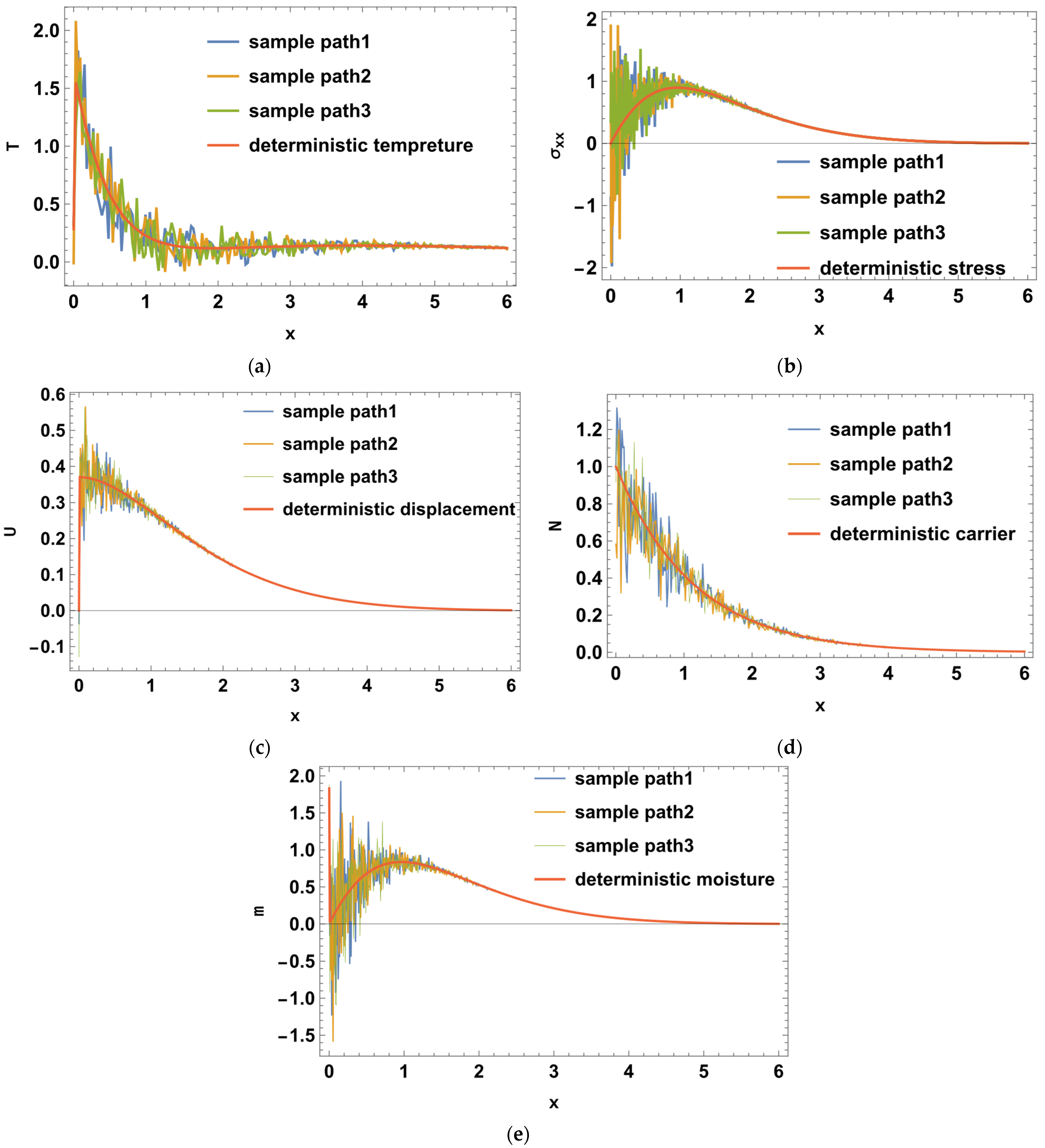
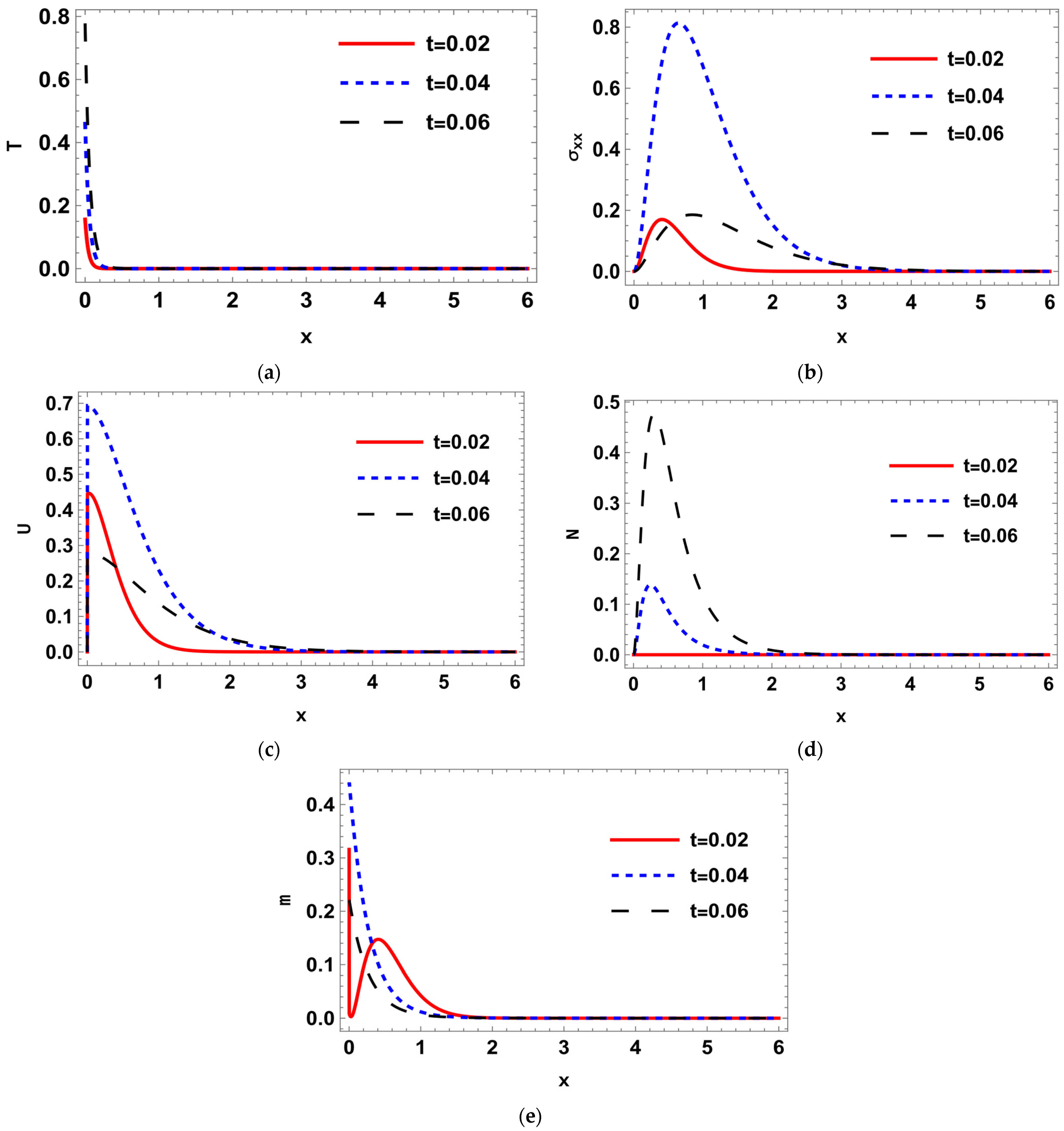
The computations were carried out numerically for various values of dimensionless times, specifically, at t = 0.02 , t = 0.04 and t = 0.06 , in order to demonstrate the theoretical results obtained from earlier parts. The calculation shows the wave propagations of thermal, normal stress, carrier (electronic) density, displacement, and moisture. The stochastic process is simulated, which displays the varying stochastic field distributions within the medium and contrast the outcomes with deterministic cases. The idea of Brownian motion or traditional Wiener processes is taken from Desmond and Hingham [18], and it is utilized to calculate the stochastic integrals necessary for the solution of physical field variables. Three sample paths of the stochastic process are taken into consideration to compare the outcomes with deterministic cases for all the physical field distributions. The solutions of the field distributions in the physical domain for both stochastic and deterministic cases are obtained in Figure 1, Figure 2 and Figure 3. Results for deterministic distributions are shown in Figure 1a–e. The results for the comparison of the deterministic case with the stochastic case are shown in Figure 2a–e. Finally, the results for the variance are shown in Figure 3a–e. Figure 1a shows the deterministic distribution of thermal wave propagation. The thermal wave distribution starts from the highest maximum point and then decreases continuously without any jumps until reaching the minimum value; then, it coincides with the zero line until it reaches the equilibrium case inside the semiconductor medium. In Figure 1b, the deterministic stress distribution begins at zero (surface), satisfying the boundary condition. When t = 0.04 and t = 0.06 , the distributions increase to maximum values, then decrease gradually to coincide with the zero minimum line. On the other hand, at t = 0.02 , the stress (mechanical) distribution decreases to the negative values with the opposite behavior of t = 0.04 and t = 0.06 , then, increases to coincide with x -axis. In Figure 1c, the deterministic case of carrier density (electronic or plasma wave) starts from a maximum value and then begins to decrease continuously in a smooth way without jumps till it disappears with increasing distance to reach the equilibrium state. In Figure 1d, at t = 0.04 and t = 0.06 the deterministic (elastic wave) displacement distribution gets started from a minimum point at zero, then increases sharply to reach the maximum value at the surface due to the thermal effect of light (the vibrations of inner particles increase), then begins to decrease gradually with exponential behavior before coinciding with the zero line. On the other side, when t = 0.02 , the wave propagation has the opposite behavior. In Figure 1d, the deterministic cases of moisture distributions, at t = 0.04 and t = 0.06 that begin from the minimum zero value at the free surface, then increase sharply to reach the maximum peak value, then decrease in exponential behavior until they coincide with the zero line (equilibrium case). Nevertheless, when t = 0.02 , it decreases sharply to the negative minimum value, then increases smoothly to coincide with the zero line [45,46,47,48,49,50].
In the second category (Figure 2a–e), Figure 2a displays a composite plot of the temperature distribution in a deterministic case and a stochastic case for three sample paths. From this figure, it is clear a great variation between the stochastic temperature distribution and the deterministic temperature distribution. Around the boundary, there is a noticeable difference between the deterministic and stochastic distributions over distinct sample paths, which later corresponds with the deterministic distribution. Figure 2b shows a composite plot of the stress distribution for three sample paths in both the deterministic and stochastic cases. It is evident from this graphic that there is a significant difference between the deterministic stress (mechanical) distribution and the stochastic temperature distribution. The stochastic and deterministic distributions across different sample paths diverge noticeably around the boundary; this difference later corresponds to the deterministic distribution. Figure 2c shows the comparison between the deterministic electronic distributions with the stochastic one. It is evident from the figure that the distributions are not equal. However, in general, with increased distance, the stochastic plasma distribution corresponds with the deterministic plasma distribution. Figure 2d shows the elastic wave distribution that is stochastically compared to a deterministic one. Close to the border surface, there is a large fluctuation, and as one goes further into the material, the variation decreases and increases in correlation with distance. Figure 2e shows the comparison between the deterministic moisture concentration distributions with the stochastic one. It is evident from the figure that the distributions are not equal. As in Figure 2b, with increased distance, the stochastic distribution corresponds with the deterministic distribution.
Figure 3a–e shows that the curve of the variance increases about the boundary of the semiconductor medium beginning from a maximum point, and after some distance, it begins to decrease and finally coincides with the zero line (equilibrium case). Figure 3b–d about the boundary begins from zero; then increases to the highest point, then goes to zero to coincide with x -axis. From this category, all the deterministic fields distribution first differs greatly from the stochastic temperature distribution over various sample paths before they eventually coincide entirely. On the other hand, all the deterministic and stochastic field distribution is continuous overall the distance. Around the boundary, there is a noticeable difference between the deterministic and stochastic distributions over distinct sample paths, which later corresponds with the deterministic distribution.

9. Conclusions

A photo-thermoelastic problem was solved for two types of boundary conditions, namely, the deterministic and stochastic types. The white noise stochastic process was chosen as the most common type. It was found that the mean of the stochastic solution coincides with the deterministic solution for all functions considered. It was also found that the deviation of the stochastic solution from its mean decreases with the distance from the bounding plane, which is the source of the noise. The fluctuations in the solution due to the noise on the boundary travel inside the medium with a finite speed, as is the case for the deterministic waves which travel inside the medium with a finite speed. From numerical results, it is clear that all the deterministic field variables are matched with the corresponding results reported by Sherief [51], and this validates the present work. This physical-mathematical model may be utilized to raise semiconductor material manufacturing effectiveness and product quality. The examination and findings in this paper will be crucial for understanding how semiconductors like diodes and triodes are used in contemporary electronics.

Author Contributions

K.L.: conceptualization, methodology; A.A.E.-B.: software, data curation; A.A. (Abdelaala Ahmed): writing—original draft preparation; R.S.T.: supervision, visualization; A.A. (Abdulaziz Alenazi): investigation, software, validation; A.A. (Abdelaala Ahmed): writing—reviewing and editing. All authors have read and agreed to the published version of the manuscript.

Funding

This research received no external funding.

Data Availability Statement

The information applied in this research is ready from the author at request.

Acknowledgments

Not Applicable.

Conflicts of Interest

The authors have declared that no competing interests exist.

Appendix A

The coefficients of Equation (50) are:
A 11 = { ( D e H 14 H 23 H 42 D e H 13 H 24 H 42 D e H 14 H 22 H 43 + D e H 12 H 24 H 43 + D e H 13 H 22 H 44 D e H 12 H 23 H 44 ) / ( D e ( H 13 H 22 H 41 + H 14 H 22 H 41 + H 12 H 23 H 41 H 14 H 23 H 41 H 12 H 24 H 41 + H 13 H 24 H 41 + H 13 H 21 H 42 H 14 H 21 H 42 H 11 H 23 H 42 + H 14 H 23 H 42 + H 11 H 24 H 42 H 13 H 24 H 42 H 12 H 21 H 43 + H 14 H 21 H 43 + H 11 H 22 H 43 H 14 H 22 H 43 H 11 H 24 H 43 + H 12 H 24 H 43 + H 12 H 21 H 44 H 13 H 21 H 44 H 11 H 22 H 44 + H 13 H 22 H 44 + H 11 H 23 H 44 H 12 H 22 H 44 ) s ) }
A 12 = { ( H 23 H 42 ħ + H 24 H 42 ħ + H 22 H 43 ħ H 24 H 43 ħ H 22 H 44 ħ + H 23 H 44 ħ ) / ( D e ( H 13 H 22 H 41 + H 14 H 22 H 41 + H 12 H 23 H 41 H 14 H 23 H 41 H 12 H 24 H 41 + H 13 H 24 H 41 + H 13 H 21 H 42 H 14 H 21 H 42 H 11 H 23 H 42 + H 14 H 23 H 42 + H 11 H 24 H 42 H 13 H 24 H 42 H 12 H 21 H 43 + H 14 H 21 H 43 + H 11 H 22 H 43 H 14 H 22 H 43 H 11 H 24 H 43 + H 12 H 24 H 43 + H 12 H 21 H 44 H 13 H 21 H 44 H 11 H 22 H 44 + H 13 H 22 H 44 + H 11 H 23 H 44 H 12 H 23 H 44 ) s ) }
A 13 = { ( ( D e H 14 H 25 H 41 D e H 13 H 24 H 41 D e H 14 H 21 H 43 + D e H 11 H 24 H 43 + D e H 13 H 21 H 44 D e H 11 H 23 H 44 ) T 0 ) / ( D e ( H 13 H 22 H 41 H 14 H 22 H 41 H 12 H 23 H 41 + H 14 H 23 H 41 + H 12 H 24 H 41 H 13 H 24 H 41 H 13 H 21 H 42 + H 14 H 42 + H 11 H 23 H 42 H 14 H 23 H 42 H 11 H 24 H 42 + H 13 H 24 H 42 + H 12 H 21 H 43 H 14 H 21 H 43 H 11 H 22 H 43 + H 14 H 22 H 43 + H 11 H 24 H 43 H 12 H 24 H 43 H 12 H 21 H 44 + H 13 H 21 H 44 + H 11 H 22 H 44 H 13 H 22 H 44 H 11 H 23 H 44 + H 12 H 23 H 44 ) s ) }
A 14 = { ( H 23 H 41 ħ + H 24 H 41 ħ + H 21 H 43 ħ H 24 H 43 ħ H 21 H 44 ħ + H 23 H 44 ħ ) / ( D e ( H 13 H 21 H 41 H 14 H 22 H 41 H 12 H 23 H 41 + H 14 H 23 H 41 + H 12 H 24 H 41 H 13 H 24 H 41 H 13 H 21 H 42 + H 14 H 21 H 42 + H 11 H 23 H 42 H 14 H 23 H 42 H 11 H 24 H 42 + H 13 H 24 H 42 + H 12 H 21 H 43 H 14 H 21 H 43 H 11 H 22 H 43 + H 14 H 22 H 43 + H 11 H 24 H 43 H 12 H 24 H 43 H 12 H 21 H 44 + H 13 H 21 H 44 + H 11 H 22 H 44 H 13 H 22 H 44 H 11 H 23 H 44 + H 12 H 23 H 44 ) s ) }
A 15 = { ( D e H 14 H 22 H 41 D e H 12 H 24 H 41 D e H 14 H 21 H 42 - D e H 11 H 24 H 42 - D e H 12 H 21 H 44 + D e H 11 H 22 H 44 ) / ( D e ( H 13 H 22 H 41 - H 14 H 22 H 41 - H 12 H 23 H 41 + H 14 H 23 H 41 + H 12 H 24 H 41 - H 13 H 24 H 41 - H 13 H 21 H 42 + H 14 H 21 H 42 + H 11 H 23 H 42 - H 14 H 23 H 42 - H 11 H 24 H 42 + H 13 H 24 H 42 + H 12 H 21 H 43 - H 14 H 21 H 43 - H 11 H 22 H 43 + H 14 H 22 H 43 H 11 H 24 H 43 H 12 H 24 H 43 - H 12 H 21 H 44 + H 13 H 21 H 44 + H 11 H 22 H 44 H 13 H 22 H 44 - H 11 H 23 H 44 + H 12 H 23 H 44 ) s ) }
A 16 = { ( H 22 H 41 ħ - H 24 H 41 ħ - H 21 H 42 ħ + H 24 H 42 ħ + H 21 H 44 ħ - H 22 H 44 ħ ) / ( D e ( H 13 H 22 H 41 H 14 H 22 H 41 H 12 H 23 H 41 + H 14 H 23 H 41 + H 12 H 24 H 41 H 13 H 24 H 41 H 13 H 21 H 42 + H 14 H 21 H 42 + H 11 H 23 H 42 H 14 H 23 H 42 H 11 H 24 H 42 + H 13 H 24 H 42 + H 12 H 21 H 43 H 14 H 21 H 43 H 11 H 22 H 43 + H 14 H 22 H 43 + H 11 H 24 H 43 H 12 H 24 H 43 H 12 H 21 H 44 + H 13 H 21 H 44 + H 11 H 22 H 44 H 13 H 22 H 44 H 11 H 23 H 44 + H 12 H 23 H 44 ) s ) }
A 17 = { ( D e H 13 H 22 H 41 D e H 12 H 23 H 41 D e H 13 H 21 H 42 + D e H 11 H 23 H 42 + D e H 12 H 21 H 43 D e H 11 H 22 H 43 ) / ( D e ( H 13 H 22 H 41 H 14 H 22 H 41 H 12 H 23 H 41 + H 14 H 23 H 41 + H 12 H 24 H 41 H 13 H 24 H 41 H 13 H 21 H 42 + H 14 H 21 H 42 + H 11 H 23 H 42 H 14 H 23 H 42 H 11 H 24 H 42 + H 13 H 24 H 42 + H 12 H 21 H 43 H 14 H 21 H 43 H 11 H 22 H 43 + H 14 H 22 H 43 + H 11 H 24 H 43 H 12 H 24 H 43 H 12 H 21 H 44 + H 13 H 21 H 44 + H 11 H 22 H 44 H 13 H 22 H 44 H 11 H 23 H 44 + H 12 H 23 H 44 ) s ) }
A 18 = { ( H 22 H 41 ħ + H 23 H 41 ħ + H 21 H 42 ħ H 23 H 42 ħ H 21 H 43 ħ + H 22 H 43 ħ ) / ( D e ( H 13 H 22 H 41 H 14 H 22 H 41 H 12 H 23 H 41 + H 14 H 23 H 41 + H 12 H 24 H 41 H 13 H 24 H 41 H 13 H 21 H 42 + H 14 H 21 H 42 + H 11 H 23 H 42 H 14 H 23 H 42 H 11 H 24 H 42 + H 13 H 24 H 42 + H 12 H 21 H 43 H 14 H 21 H 43 H 11 H 22 H 43 + H 14 H 22 H 43 + H 11 H 24 H 43 H 12 H 24 H 43 H 12 H 21 H 44 + H 13 H 21 H 44 + H 11 H 22 H 44 H 13 H 22 H 44 H 11 H 23 H 44 + H 12 H 23 H 44 ) s ) }
The coefficients of Equation (68) are:
E 11 = { H 41 ( D E H 14 H 23 H 42 D E H 13 H 24 H 42 D E H 14 H 22 H 43 + D E H 12 H 24 H 43 + D E H 13 H 22 H 44 D E H 12 H 23 H 44 ) / ( D E ( H 13 H 22 H 41 + H 14 H 22 H 41 + H 12 H 23 H 41 - H 14 H 23 H 41 - H 12 H 24 H 41 + H 13 H 24 H 41 + H 13 H 21 H 42 - H 14 H 21 H 42 - H 11 H 23 H 42 + H 14 H 23 H 42 + H 11 H 24 H 42 - H 13 H 24 H 42 - H 12 H 21 H 43 + H 14 H 21 H 43 + H 11 H 22 H 43 - H 14 H 22 H 43 - H 11 H 24 H 43 + H 12 H 24 H 43 + H 12 H 21 H 44 - H 13 H 21 H 44 - H 11 H 22 H 44 + H 13 H 22 H 44 + H 11 H 23 H 44 - H 12 H 23 H 44 ) s ) }
E 12 = { ( H 41 ( - H 23 H 42 ħ + H 24 H 42 ħ + H 22 H 43 ħ - H 24 H 43 ħ - H 22 H 44 ħ + H 23 H 44 ħ ) / ( D E ( - H 13 H 22 H 41 + H 14 H 22 H 41 + H 12 H 23 H 41 - H 14 H 23 H 41 - H 12 H 24 H 41 + H 13 H 24 H 41 + H 13 H 21 H 42 - H 14 H 21 H 42 - H 11 H 23 H 42 + H 14 H 23 H 42 + H 11 H 24 H 42 - H 13 H 24 H 42 - H 12 H 21 H 43 + H 14 H 21 H 43 + H 11 H 22 H 43 - H 14 H 22 H 43 - H 11 H 24 H 43 + H 12 H 24 H 43 + H 12 H 21 H 44 - H 13 H 21 H 44 - H 11 H 22 H 44 + H 13 H 22 H 44 + H 11 H 23 H 44 - H 12 H 23 H 44 ) s ) }
E 13 = { H 42 ( D E H 14 H 23 H 41 D E H 13 H 24 H 41 D E H 14 H 21 H 43 + D E H 11 H 24 H 43 + D E H 13 H 21 H 44 D E H 11 H 23 H 44 ) / ( D E ( H 13 H 22 H 41 - H 14 H 22 H 41 - H 12 H 23 H 41 + H 14 H 23 H 41 + H 12 H 24 H 41 - H 13 H 24 H 41 - H 13 H 21 H 42 + H 14 H 21 H 42 + H 11 H 23 H 42 - H 14 H 23 H 42 - H 11 H 24 H 42 + H 13 H 24 H 42 + H 12 H 21 H 43 - H 14 H 21 H 43 - H 11 H 22 H 43 + H 14 H 22 H 43 + H 11 H 24 H 43 - H 12 H 24 H 43 - H 12 H 21 H 44 + H 13 H 21 H 44 + H 11 H 22 H 44 - H 13 H 22 H 44 - H 11 H 23 H 44 + H 12 H 23 H 44 ) s ) }
E 14 = { ( H 42 ( - H 23 H 41 ħ + H 24 H 42 ħ + H 21 H 43 ħ - H 24 H 43 ħ - H 21 H 44 ħ + H 23 H 44 ħ ) / ( D E ( H 13 H 22 H 41 - H 14 H 22 H 41 - H 12 H 23 H 41 + H 14 H 23 H 41 + H 12 H 24 H 41 - H 13 H 24 H 41 - H 13 H 21 H 42 + H 14 H 21 H 42 + H 11 H 23 H 42 - H 14 H 23 H 42 - H 11 H 24 H 42 + H 13 H 24 H 42 + H 12 H 21 H 43 - H 14 H 21 H 43 - H 11 H 22 H 43 + H 14 H 22 H 43 + H 11 H 24 H 43 - H 12 H 24 H 43 - H 12 H 21 H 44 + H 13 H 21 H 44 + H 11 H 22 H 44 - H 13 H 22 H 44 - H 11 H 23 H 44 + H 12 H 23 H 44 ) s ) }
E 15 = { H 43 ( - D E H 14 H 22 H 41 + D E H 12 H 24 H 41 + D E H 14 H 21 H 42 - D E H 11 H 24 H 42 - D E H 12 H 21 H 44 + D E H 11 H 22 H 44 ) / ( D E ( H 13 H 22 H 41 - H 14 H 22 H 41 - H 12 H 23 H 41 + H 14 H 23 H 41 + H 12 H 24 H 41 - H 13 H 24 H 41 - H 13 H 21 H 42 + H 14 H 21 H 42 + H 11 H 23 H 42 - H 14 H 23 H 42 - H 11 H 24 H 42 + H 13 H 24 H 42 + H 12 H 21 H 43 - H 14 H 21 H 43 - H 11 H 22 H 43 + H 14 H 22 H 43 + H 11 H 24 H 43 - H 12 H 24 H 43 - H 12 H 21 H 44 + H 13 H 21 H 44 + H 11 H 22 H 44 - H 13 H 22 H 44 - H 11 H 23 H 44 + H 12 H 23 H 44 ) s ) }
E 16 = { H 43 H 22 H 41 ħ H 24 H 41 ħ H 21 H 42 ħ + H 24 H 42 ħ + H 21 H 44 ħ H 22 H 44 ħ / ( D E ( H 13 H 22 H 41 H 14 H 22 H 41 H 12 H 23 H 41 + H 14 H 23 H 41 + H 12 H 24 H 41 H 13 H 24 H 41 H 13 H 21 H 42 + H 14 H 21 H 42 + H 11 H 23 H 42 H 14 H 23 H 42 H 11 H 24 H 42 + H 13 H 24 H 42 + H 12 H 21 H 43 H 14 H 21 H 43 H 11 H 22 H 43 + H 14 H 22 H 43 + H 11 H 24 H 43 H 12 H 24 H 43 H 12 H 21 H 44 + H 13 H 21 H 44 + H 11 H 22 H 44 H 13 H 22 H 44 H 11 H 23 H 44 + H 12 H 23 H 44 ) s ) }
E 17 = { D E H 13 H 22 H 41 D E H 12 H 23 H 41 D E H 13 H 21 H 42 + D E H 11 H 23 H 42 + D E H 12 H 21 H 43 D E H 11 H 22 H 43 H 44 / ( D E ( H 13 H 22 H 41 H 14 H 22 H 41 H 12 H 23 H 41 + H 14 H 23 H 41 + H 12 H 24 H 41 H 13 H 24 H 41 H 13 H 21 H 42 + H 14 H 21 H 42 + H 11 H 23 H 42 H 14 H 23 H 42 H 11 H 24 H 42 + H 13 H 24 H 42 + H 12 H 21 H 43 H 14 H 21 H 43 H 11 H 22 H 43 + H 14 H 22 H 43 + H 11 H 24 H 43 H 12 H 24 H 43 H 12 H 21 H 44 + H 13 H 21 H 44 + H 11 H 22 H 44 H 13 H 22 H 44 H 11 H 23 H 44 + H 12 H 23 H 44 ) s ) }
E 18 = { H 44 H 22 H 41 ħ + H 23 H 41 ħ + H 21 H 42 ħ H 23 H 42 ħ H 21 H 43 ħ + H 22 H 43 ħ / ( D E ( H 13 H 22 H 41 H 14 H 22 H 41 H 12 H 23 H 41 + H 14 H 23 H 41 + H 12 H 24 H 41 H 13 H 24 H 41 H 13 H 21 H 42 + H 14 H 21 H 42 + H 11 H 23 H 42 H 14 H 23 H 42 H 11 H 24 H 42 + H 13 H 24 H 42 + H 12 H 21 H 43 H 14 H 21 H 43 H 11 H 22 H 43 + H 14 H 22 H 43 + H 11 H 24 H 43 H 12 H 24 H 43 H 12 H 21 H 44 + H 13 H 21 H 44 + H 11 H 22 H 44 H 13 H 22 H 44 H 11 H 23 H 44 + H 12 H 23 H 44 ) s ) }
The coefficients of Equation (76) are:
D 11 = { H 21 D E H 14 H 23 H 42 D E H 13 H 24 H 42 D E H 14 H 22 H 43 + D E H 12 H 24 H 43 + D E H 13 H 22 H 44 D E H 12 H 23 H 44 / ( D E ( H 13 H 22 H 41 + H 14 H 22 H 41 + H 12 H 23 H 41 H 14 H 23 H 41 H 12 H 24 H 41 + H 13 H 24 H 41 + H 13 H 21 H 42 H 14 H 21 H 42 H 11 H 23 H 42 + H 14 H 23 H 42 + H 11 H 24 H 42 H 13 H 24 H 42 H 12 H 21 H 43 + H 14 H 21 H 43 + H 11 H 22 H 43 H 14 H 22 H 43 H 11 H 24 H 43 + H 12 H 24 H 43 + H 12 H 21 H 44 H 13 H 21 H 44 H 11 H 22 H 44 + H 13 H 22 H 44 + H 11 H 23 H 44 H 12 H 23 H 44 ) s ) }
D 12 = { H 21 H 23 H 42 ħ + H 24 H 42 ħ + H 22 H 43 ħ H 24 H 43 ħ H 22 H 44 ħ + H 23 H 44 ħ / ( D E ( H 13 H 22 H 41 + H 14 H 22 H 41 + H 12 H 23 H 41 H 14 H 23 H 41 H 12 H 24 H 41 + H 13 H 24 H 41 + H 13 H 21 H 42 H 14 H 21 H 42 H 11 H 23 H 42 + H 14 H 23 H 42 + H 11 H 24 H 42 H 13 H 24 H 42 H 12 H 21 H 43 + H 14 H 21 H 43 + H 11 H 22 H 43 H 14 H 22 H 43 H 11 H 24 H 43 + H 12 H 24 H 43 + H 12 H 21 H 44 H 13 H 21 H 44 H 11 H 22 H 44 + H 13 H 22 H 44 + H 11 H 23 H 44 H 12 H 23 H 44 ) s ) }
D 13 = { H 22 D E H 14 H 23 H 41 D E H 13 H 24 H 41 D E H 14 H 21 H 43 + D E H 11 H 24 H 43 + D E H 13 H 21 H 44 D E H 11 H 23 H 44 / ( D E ( H 13 H 22 H 41 H 14 H 22 H 41 H 12 H 23 H 41 + H 14 H 23 H 41 + H 12 H 24 H 41 H 13 H 24 H 41 H 13 H 21 H 42 + H 14 H 21 H 42 + H 11 H 23 H 42 H 14 H 23 H 42 H 11 H 24 H 42 + H 13 H 24 H 42 + H 12 H 21 H 43 H 14 H 21 H 43 H 11 H 22 H 43 + H 14 H 22 H 43 + H 11 H 24 H 43 H 12 H 24 H 43 H 12 H 21 H 44 + H 13 H 21 H 44 + H 11 H 22 H 44 H 13 H 22 H 44 H 11 H 23 H 44 + H 12 H 23 H 44 ) s ) }
D 14 = { H 22 H 23 H 41 ħ + H 24 H 41 ħ + H 21 H 43 ħ H 24 H 43 ħ H 21 H 44 ħ + H 23 H 44 ħ / ( D E ( H 13 H 22 H 41 H 14 H 22 H 41 H 12 H 23 H 41 + H 14 H 23 H 41 + H 12 H 24 H 41 H 13 H 24 H 41 H 13 H 21 H 42 + H 14 H 21 H 42 + H 11 H 23 H 42 H 14 H 23 H 42 H 11 H 24 H 42 + H 13 H 24 H 42 + H 12 H 21 H 43 H 14 H 21 H 43 H 11 H 22 H 43 + H 14 H 22 H 43 + H 11 H 24 H 43 H 12 H 24 H 43 H 12 H 21 H 44 + H 13 H 21 H 44 + H 11 H 22 H 44 H 13 H 22 H 44 H 11 H 23 H 44 + H 12 H 23 H 44 ) s ) }
D 15 = { H 23 D E H 14 H 22 H 41 + D E H 12 H 24 H 41 + D E H 14 H 21 H 42 D E H 11 H 24 H 42 D E H 12 H 21 H 44 + D E H 11 H 22 H 44 / ( D E ( H 13 H 22 H 41 H 14 H 22 H 41 H 12 H 23 H 41 + H 14 H 23 H 41 + H 12 H 24 H 41 H 13 H 24 H 41 H 13 H 21 H 42 + H 14 H 21 H 42 + H 11 H 23 H 42 H 14 H 23 H 42 H 11 H 24 H 42 + H 13 H 24 H 42 + H 12 H 21 H 43 H 14 H 21 H 43 H 11 H 22 H 43 + H 14 H 22 H 43 + H 11 H 24 H 43 H 12 H 24 H 43 H 12 H 21 H 44 + H 13 H 21 H 44 + H 11 H 22 H 44 H 13 H 22 H 44 H 11 H 23 H 44 + H 12 H 23 H 44 ) s ) }
D 16 = { H 23 H 22 H 41 ħ H 24 H 41 ħ H 21 H 42 ħ + H 24 H 42 ħ + H 21 H 44 ħ H 22 H 44 ħ / ( D E ( H 13 H 22 H 41 H 14 H 22 H 41 H 12 H 23 H 41 + H 14 H 23 H 41 + H 12 H 24 H 41 H 13 H 24 H 41 H 13 H 21 H 42 + H 14 H 21 H 42 + H 11 H 23 H 42 H 14 H 23 H 42 H 11 H 24 H 42 + H 13 H 24 H 42 + H 12 H 21 H 43 H 14 H 21 H 43 H 11 H 22 H 43 + H 14 H 22 H 43 + H 11 H 24 H 43 H 12 H 24 H 43 H 12 H 21 H 44 + H 13 H 21 H 44 + H 11 H 22 H 44 H 13 H 22 H 44 H 11 H 23 H 44 + H 12 H 23 H 44 ) s ) }
D 17 = { H 24 D E H 13 H 22 H 41 D E H 12 H 23 H 41 D E H 13 H 21 H 42 + D E H 11 H 23 H 42 + D E H 12 H 21 H 43 D E H 11 H 22 H 43 / ( D E ( H 13 H 22 H 41 H 14 H 22 H 41 H 12 H 23 H 41 + H 14 H 23 H 41 + H 12 H 24 H 41 H 13 H 24 H 41 H 13 H 21 H 42 + H 14 H 21 H 42 + H 11 H 23 H 42 H 14 H 23 H 42 H 11 H 24 H 42 + H 13 H 24 H 42 + H 12 H 21 H 43 H 14 H 21 H 43 H 11 H 22 H 43 + H 14 H 22 H 43 + H 11 H 24 H 43 H 12 H 24 H 43 H 12 H 21 H 44 + H 13 H 21 H 44 + H 11 H 22 H 44 H 13 H 22 H 44 H 11 H 23 H 44 + H 12 H 23 H 44 ) s ) }
D 18 = { H 24 H 22 H 41 ħ + H 23 H 41 ħ + H 21 H 42 ħ H 23 H 42 ħ H 21 H 43 ħ + H 22 H 43 ħ / ( D E ( H 13 H 22 H 41 H 14 H 22 H 41 H 12 H 23 H 41 + H 14 H 23 H 41 + H 12 H 24 H 41 H 13 H 24 H 41 H 13 H 21 H 42 + H 14 H 21 H 42 + H 11 H 23 H 42 H 14 H 23 H 42 H 11 H 24 H 42 + H 13 H 24 H 42 + H 12 H 21 H 43 H 14 H 21 H 43 H 11 H 22 H 43 + H 14 H 22 H 43 + H 11 H 24 H 43 H 12 H 24 H 43 H 12 H 21 H 44 + H 13 H 21 H 44 + H 11 H 22 H 44 H 13 H 22 H 44 H 11 H 23 H 44 + H 12 H 23 H 44 ) s ) }
The coefficients of Equation (84) are:
B 11 = { H 11 D E H 14 H 23 H 42 D E H 13 H 24 H 42 D E H 14 H 22 H 43 + D E H 12 H 24 H 43 + D E H 13 H 22 H 44 D E H 12 H 23 H 44 / ( D E ( H 13 H 22 H 41 + H 14 H 22 H 41 + H 12 H 23 H 41 H 14 H 23 H 41 H 12 H 24 H 41 + H 13 H 24 H 41 + H 13 H 21 H 42 H 14 H 21 H 42 H 11 H 23 H 42 + H 14 H 23 H 42 + H 11 H 24 H 42 H 13 H 24 H 42 H 12 H 21 H 43 + H 14 H 21 H 43 + H 11 H 22 H 43 H 14 H 22 H 43 H 11 H 24 H 43 + H 12 H 24 H 43 + H 12 H 21 H 44 H 13 H 21 H 44 H 11 H 22 H 44 + H 13 H 22 H 44 + H 11 H 23 H 44 H 12 H 23 H 44 ) s ) }
B 12 = { H 11 H 23 H 42 ħ + H 24 H 42 ħ + H 22 H 43 ħ H 24 H 43 ħ H 22 H 44 ħ + H 23 H 44 ħ / ( D E ( H 13 H 22 H 41 + H 14 H 22 H 41 + H 12 H 23 H 41 H 14 H 23 H 41 H 12 H 24 H 41 + H 13 H 24 H 41 + H 13 H 21 H 42 H 14 H 21 H 42 H 11 H 23 H 42 + H 14 H 23 H 42 + H 11 H 24 H 42 H 13 H 24 H 42 H 12 H 21 H 43 + H 14 H 21 H 43 + H 11 H 22 H 43 H 14 H 22 H 43 H 11 H 24 H 43 + H 12 H 24 H 43 + H 12 H 21 H 44 H 13 H 21 H 44 H 11 H 22 H 44 + H 13 H 22 H 44 + H 11 H 23 H 44 H 12 H 23 H 44 ) s ) }
B 13 = { H 12 D E H 14 H 23 H 41 D E H 13 H 24 H 41 D E H 14 H 21 H 43 + D E H 11 H 24 H 43 + D E H 13 H 21 H 44 D E H 11 H 23 H 44 / ( D E ( H 13 H 22 H 41 H 14 H 22 H 41 H 12 H 23 H 41 + H 14 H 23 H 41 + H 12 H 24 H 41 H 13 H 24 H 41 H 13 H 21 H 42 + H 14 H 21 H 42 + H 11 H 23 H 42 H 14 H 23 H 42 H 11 H 24 H 42 + H 13 H 24 H 42 + H 12 H 21 H 43 H 14 H 21 H 43 H 11 H 22 H 43 + H 14 H 22 H 43 + H 11 H 24 H 43 H 12 H 24 H 43 H 12 H 21 H 44 + H 13 H 21 H 44 + H 11 H 22 H 44 H 13 H 22 H 44 H 11 H 23 H 44 + H 12 H 23 H 44 ) s ) }
B 14 = { H 12 H 23 H 41 ħ + H 24 H 41 ħ + H 21 H 43 ħ H 24 H 43 ħ H 21 H 44 ħ + H 23 H 44 ħ / ( D E ( H 13 H 22 H 41 H 14 H 22 H 41 H 12 H 23 H 41 + H 14 H 23 H 41 + H 12 H 24 H 41 H 13 H 24 H 41 H 13 H 21 H 42 + H 14 H 21 H 42 + H 11 H 23 H 42 H 14 H 23 H 42 H 11 H 24 H 42 + H 13 H 24 H 42 + H 12 H 21 H 43 H 14 H 21 H 43 H 11 H 22 H 43 + H 14 H 22 H 43 + H 11 H 24 H 43 H 12 H 24 H 43 H 12 H 21 H 44 + H 13 H 21 H 44 + H 11 H 22 H 44 H 13 H 22 H 44 H 11 H 23 H 44 + H 12 H 23 H 44 ) s ) }
B 15 = { H 13 D E H 14 H 22 H 41 + D E H 12 H 24 H 41 + D E H 14 H 21 H 42 D E H 11 H 24 H 42 D E H 12 H 21 H 44 + D E H 11 H 22 H 44 / ( D E ( H 13 H 22 H 41 H 14 H 22 H 41 H 12 H 23 H 41 + H 14 H 23 H 41 + H 12 H 24 H 41 H 13 H 24 H 41 H 13 H 21 H 42 + H 14 H 21 H 42 + H 11 H 23 H 42 H 14 H 23 H 42 H 11 H 24 H 42 + H 13 H 24 H 42 + H 12 H 21 H 43 H 14 H 21 H 43 H 11 H 22 H 43 + H 14 H 22 H 43 + H 11 H 24 H 43 H 12 H 24 H 43 H 12 H 21 H 44 + H 13 H 21 H 44 + H 11 H 22 H 44 H 13 H 22 H 44 H 11 H 23 H 44 + H 12 H 23 H 44 ) s ) }
B 16 = { H 13 H 22 H 41 ħ - H 24 H 41 ħ - H 21 H 42 ħ + H 24 H 42 ħ + H 21 H 44 ħ - H 22 H 44 ħ / ( D E ( H 13 H 22 H 41 H 14 H 22 H 41 H 12 H 23 H 41 + H 14 H 23 H 41 + H 12 H 24 H 41 H 13 H 24 H 41 H 13 H 21 H 42 + H 14 H 21 H 42 + H 11 H 23 H 42 H 14 H 23 H 42 H 11 H 24 H 42 + H 13 H 24 H 42 + H 12 H 21 H 43 H 14 H 21 H 43 H 11 H 22 H 43 + H 14 H 22 H 43 + H 11 H 24 H 43 H 12 H 24 H 43 H 12 H 21 H 44 + H 13 H 21 H 44 + H 11 H 22 H 44 H 13 H 22 H 44 H 11 H 23 H 44 + H 12 H 23 H 44 ) s ) }
B 17 = { H 14 D E H 13 H 22 H 41 D E H 12 H 23 H 41 D E H 13 H 21 H 42 + D E H 11 H 23 H 42 + D E H 12 H 21 H 43 D E H 11 H 22 H 43 / ( D E ( H 13 H 22 H 41 H 14 H 22 H 41 H 12 H 23 H 41 + H 14 H 23 H 41 + H 12 H 24 H 41 H 13 H 24 H 41 H 13 H 21 H 42 + H 14 H 21 H 42 + H 11 H 23 H 42 H 14 H 23 H 42 H 11 H 24 H 42 + H 13 H 24 H 42 + H 12 H 21 H 43 H 14 H 21 H 43 H 11 H 22 H 43 + H 14 H 22 H 43 + H 11 H 24 H 43 H 12 H 24 H 43 H 12 H 21 H 44 + H 13 H 21 H 44 + H 11 H 22 H 44 H 13 H 22 H 44 H 11 H 23 H 44 + H 12 H 23 H 44 ) s ) }
B 18 = { H 14 H 22 H 41 ħ + H 23 H 41 ħ + H 21 H 42 ħ H 23 H 42 ħ H 21 H 43 ħ + H 22 H 43 ħ / ( D E ( H 13 H 22 H 41 H 14 H 22 H 41 H 12 H 23 H 41 + H 14 H 23 H 41 + H 12 H 24 H 41 H 13 H 24 H 41 H 13 H 21 H 42 + H 14 H 21 H 42 + H 11 H 23 H 42 H 14 H 23 H 42 H 11 H 24 H 42 + H 13 H 24 H 42 + H 12 H 21 H 43 H 14 H 21 H 43 H 11 H 22 H 43 + H 14 H 22 H 43 + H 11 H 24 H 43 H 12 H 24 H 43 H 12 H 21 H 44 + H 13 H 21 H 44 + H 11 H 22 H 44 H 13 H 22 H 44 H 11 H 23 H 44 + H 12 H 23 H 44 ) s ) }
The coefficients of Equation (92) are:
C 11 = { H 31 D E H 14 H 23 H 42 - D E H 13 H 24 H 42 - D E H 14 H 22 H 43 + D E H 12 H 24 H 43 + D E H 13 H 22 H 44 - D E H 12 H 23 H 44 / ( D E ( - H 13 H 22 H 41 + H 14 H 22 H 41 + H 12 H 23 H 41 - H 14 H 23 H 41 - H 12 H 24 H 41 + H 13 H 24 H 41 + H 13 H 21 H 42 - H 14 H 21 H 42 - H 11 H 23 H 42 + H 14 H 23 H 42 + H 11 H 24 H 42 - H 13 H 24 H 42 - H 12 H 21 H 43 + H 14 H 21 H 43 + H 11 H 22 H 43 - H 14 H 22 H 43 - H 11 H 24 H 43 + H 12 H 24 H 43 + H 12 H 21 H 44 - H 13 H 21 H 44 - H 11 H 22 H 44 + H 13 H 22 H 44 + H 11 H 23 H 44 - H 12 H 23 H 44 ) s ) }
C 12 = { H 31 H 23 H 42 ħ + H 24 H 42 ħ + H 22 H 43 ħ H 24 H 43 ħ H 22 H 44 ħ + H 23 H 44 ħ / ( D E ( H 13 H 22 H 41 + H 14 H 22 H 41 + H 12 H 23 H 41 H 14 H 23 H 41 H 12 H 24 H 41 + H 13 H 24 H 41 + H 13 H 21 H 42 H 14 H 21 H 42 H 11 H 23 H 42 + H 14 H 23 H 42 + H 11 H 24 H 42 H 13 H 24 H 42 H 12 H 21 H 43 + H 14 H 21 H 43 + H 11 H 22 H 43 H 14 H 22 H 43 H 11 H 24 H 43 + H 12 H 24 H 43 + H 12 H 21 H 44 H 13 H 21 H 44 H 11 H 22 H 44 + H 13 H 22 H 44 + H 11 H 23 H 44 H 12 H 23 H 44 ) s ) }
C 13 = { H 32 D E H 14 H 23 H 41 D E H 13 H 24 H 41 D E H 14 H 21 H 43 + D E H 11 H 24 H 43 + D E H 13 H 21 H 44 D E H 11 H 23 H 44 / ( D E ( H 13 H 22 H 41 H 14 H 22 H 41 H 12 H 23 H 41 + H 14 H 23 H 41 + H 12 H 24 H 41 H 13 H 24 H 41 H 13 H 21 H 42 + H 14 H 21 H 42 + H 11 H 23 H 42 H 14 H 23 H 42 H 11 H 24 H 42 + H 13 H 24 H 42 + H 12 H 21 H 43 H 14 H 21 H 43 H 11 H 22 H 43 + H 14 H 22 H 43 + H 11 H 24 H 43 H 12 H 24 H 43 H 12 H 21 H 44 + H 13 H 21 H 44 + H 11 H 22 H 44 H 13 H 22 H 44 H 11 H 23 H 44 + H 12 H 23 H 44 ) s ) }
C 14 = { H 32 H 23 H 41 ħ + H 24 H 41 ħ + H 21 H 43 ħ H 24 H 43 ħ H 21 H 44 ħ + H 23 H 44 ħ / ( D E ( H 13 H 22 H 41 H 14 H 22 H 41 H 12 H 23 H 41 + H 14 H 23 H 41 + H 12 H 24 H 41 H 13 H 24 H 41 H 13 H 21 H 42 + H 14 H 21 H 42 + H 11 H 23 H 42 H 14 H 23 H 42 H 11 H 24 H 42 + H 13 H 24 H 42 + H 12 H 21 H 43 H 14 H 21 H 43 H 11 H 22 H 43 + H 14 H 22 H 43 + H 11 H 24 H 43 H 12 H 24 H 43 H 12 H 21 H 44 + H 13 H 21 H 44 + H 11 H 22 H 44 H 13 H 22 H 44 H 11 H 23 H 44 + H 12 H 23 H 44 ) s ) }
C 15 = { H 33 D E H 14 H 22 H 41 + D E H 12 H 24 H 41 + D E H 14 H 21 H 42 D E H 11 H 24 H 42 D E H 12 H 21 H 44 + D E H 11 H 22 H 44 / ( D E ( H 13 H 22 H 41 H 14 H 22 H 41 H 12 H 23 H 41 + H 14 H 23 H 41 + H 12 H 24 H 41 H 13 H 24 H 41 H 13 H 21 H 42 + H 14 H 21 H 42 + H 11 H 23 H 42 H 14 H 23 H 42 H 11 H 24 H 42 + H 13 H 24 H 42 + H 12 H 21 H 43 H 14 H 21 H 43 H 11 H 22 H 43 + H 14 H 22 H 43 + H 11 H 24 H 43 H 12 H 24 H 43 H 12 H 21 H 44 + H 13 H 21 H 44 + H 11 H 22 H 44 H 13 H 22 H 44 H 11 H 23 H 44 + H 12 H 23 H 44 ) s ) }
C 16 = { H 33 H 22 H 41 ħ H 24 H 41 ħ H 21 H 42 ħ + H 24 H 42 ħ + H 21 H 44 ħ H 22 H 44 ħ / ( D E ( H 13 H 22 H 41 H 14 H 22 H 41 H 12 H 23 H 41 + H 14 H 23 H 41 + H 12 H 24 H 41 H 13 H 24 H 41 H 13 H 21 H 42 + H 14 H 21 H 42 + H 11 H 23 H 42 H 14 H 23 H 42 H 11 H 24 H 42 + H 13 H 24 H 42 + H 12 H 21 H 43 H 14 H 21 H 43 H 11 H 22 H 43 + H 14 H 22 H 43 + H 11 H 24 H 43 H 12 H 24 H 43 H 12 H 21 H 44 + H 13 H 21 H 44 + H 11 H 22 H 44 H 13 H 22 H 44 H 11 H 23 H 44 + H 12 H 23 H 44 ) s ) }
C 17 = { H 34 D E H 13 H 22 H 41 D E H 12 H 23 H 41 D E H 13 H 21 H 42 + D E H 11 H 23 H 42 + D E H 12 H 21 H 43 D E H 11 H 22 H 43 / ( D E ( H 13 H 22 H 41 H 14 H 22 H 41 H 12 H 23 H 41 + H 14 H 23 H 41 + H 12 H 24 H 41 H 13 H 24 H 41 H 13 H 21 H 42 + H 14 H 21 H 42 + H 11 H 23 H 42 H 14 H 23 H 42 H 11 H 24 H 42 + H 13 H 24 H 42 + H 12 H 21 H 43 H 14 H 21 H 43 H 11 H 22 H 43 + H 14 H 22 H 43 + H 11 H 24 H 43 H 12 H 24 H 43 H 12 H 21 H 44 + H 13 H 21 H 44 + H 11 H 22 H 44 H 13 H 22 H 44 H 11 H 23 H 44 + H 12 H 23 H 44 ) s ) }
C 18 = { H 34 H 22 H 41 ħ + H 23 H 41 ħ + H 21 H 42 ħ H 23 H 42 ħ H 21 H 43 ħ + H 22 H 43 ħ / ( D E ( H 13 H 22 H 41 H 14 H 22 H 41 H 12 H 23 H 41 + H 14 H 23 H 41 + H 12 H 24 H 41 H 13 H 24 H 41 H 13 H 21 H 42 + H 14 H 21 H 42 + H 11 H 23 H 42 H 14 H 23 H 42 H 11 H 24 H 42 + H 13 H 24 H 42 + H 12 H 21 H 43 H 14 H 21 H 43 H 11 H 22 H 43 + H 14 H 22 H 43 + H 11 H 24 H 43 H 12 H 24 H 43 H 12 H 21 H 44 + H 13 H 21 H 44 + H 11 H 22 H 44 H 13 H 22 H 44 H 11 H 23 H 44 + H 12 H 23 H 44 ) s ) }

References

  1. Biot, M. Thermoelasticity and irreversible thermodynamics. J. Appl. Phys. 1956, 27, 240–253. [Google Scholar] [CrossRef]
  2. Lord, H.; Shulman, Y. A generalized dynamical theory of thermoelasticity. J. Mech. Phys. Solids 1967, 15, 299–309. [Google Scholar] [CrossRef]
  3. Green, A.; Lindsay, K. Thermoelasticity. J. Elast. 1972, 2, 1–7. [Google Scholar] [CrossRef]
  4. Lebon, D.J.G.; Casas-Vzquez, J. Understanding Non-Equilibrium Thermodynamics: Foundations, Applications, Frontiers; Springer: Berlin/Heidelberg, Germany, 2008. [Google Scholar]
  5. Maurer, M.J.; Thompson, H.A. Non-fourier effects at high heat flux. J. Heat Transf. 1973, 95, 284–286. [Google Scholar] [CrossRef]
  6. Sherief, H.H.; Dhliwal, R.S. Generalized one-dimensional thermal-shock problem for small times. J. Therm. Stress. 1981, 4, 407–420. [Google Scholar] [CrossRef]
  7. Marin, M. Harmonic vibrations in thermoelasticity of microstretch materials, journal of vibration and acoustics. Trans. ASME 2010, 132, 044501. [Google Scholar]
  8. Marin, M.; Othman, M.; Abbas, I. An extension of the domain of influence theorem for generalized thermoelasticity of anisotropic material with voids. J. Comp. Theor. Nanosci. 2015, 12, 1594–1598. [Google Scholar] [CrossRef]
  9. Othman, M.; Lotfy, K. On the plane waves of generalized thermo-microstretch elastic half-space under three theories. Int. Comm. Heat Mass Trans. 2010, 37, 192–200. [Google Scholar] [CrossRef]
  10. Abouelregal, A.; Marin, M. The Size-Dependent Thermoelastic Vibrations of Nanobeams Subjected to Harmonic Excitation and Rectified Sine Wave Heating. Mathematics 2020, 8, 1128. [Google Scholar] [CrossRef]
  11. Othman, M.; Lotfy, K. Effect of rotating on plane waves in generalized thermo-microstretch elastic solid with one relaxation time, Multidis. Model. Mat. Struct. 2011, 7, 43–62. [Google Scholar] [CrossRef]
  12. Ailawalia, P.; Sachdeva, S.; Pathania, D. Plane strain deformation in a thermo-elastic microelongated solid with internal heat source. Int. J. Appl. Mech. Eng. 2015, 20, 717–731. [Google Scholar] [CrossRef]
  13. Todorovic, D.; Nikolic, P.; Bojic, A. Photoacoustic frequency transmission technique: Electronic deformation mechanism in semiconductors. J. Appl. Phys. 1999, 85, 7716–7726. [Google Scholar] [CrossRef]
  14. Todorovic, D. Plasma, thermal, and elastic waves in semiconductors. Rev. Sci. Instrum. 2003, 74, 582–591. [Google Scholar] [CrossRef]
  15. Gordon, J.P.; Leite, R.C.C.; Moore, R.S.; Porto, S.P.S.; Whinnery, J.R. Long-transient effects in lasers with inserted liquid samples. Bull. Am. Phys. Soc. 1964, 119, 501–510. [Google Scholar] [CrossRef]
  16. Kreuzer, L.B. Ultralow gas concentration infrared absorption spectroscopy. J. Appl. Phys. 1971, 42, 2934. [Google Scholar] [CrossRef]
  17. Tam, A.C. Ultrasensitive Laser Spectroscopy; Academic Press: New York, NY, USA, 1983; pp. 1–108. [Google Scholar]
  18. Tam, A.C. Applications of photoacoustic sensing techniques. Rev. Mod. Phys. 1986, 58, 381. [Google Scholar] [CrossRef]
  19. Hobiny, A.; Abbas, I. A GN model on photothermal interactions in a two-dimensions semiconductor half space. Results Phys. 2019, 15, 102588. [Google Scholar] [CrossRef]
  20. Lotfy, K. A Novel Model of Photothermal Diffusion (PTD) for Polymer Nano- composite Semiconducting of Thin Circular Plate. Phys. B-Condenced Matter 2018, 537, 320–328. [Google Scholar] [CrossRef]
  21. Lotfy, K.; Kumar, R.; Hassan, W.; Gabr, M. Thermomagnetic effect with microtemperature in a semiconducting Photothermal excitation medium. Appl. Math. Mech. Engl. Ed. 2018, 39, 783–796. [Google Scholar] [CrossRef]
  22. Lotfy, K. A novel model for Photothermal excitation of variable thermal conductivity semiconductor elastic medium subjected to mechanical ramp type with two-temperature theory and magnetic field. Sci. Rep. 2019, 9, 3319. [Google Scholar] [CrossRef]
  23. Abbas, I.; Alzahranib, F.; Elaiwb, A. A DPL model of photothermal interaction in a semiconductor material, Waves Rand. Comp. Media 2019, 29, 328–343. [Google Scholar]
  24. Khamis, A.; El-Bary, A.; Lotfy, K.; Bakali, A. Photothermal excitation processes with refined multi dual phase-lags theory for semiconductor elastic medium. Alex. Eng. J. 2020, 59, 1–9. [Google Scholar] [CrossRef]
  25. Lotfy, K.; El-Bary, A.; El-Sharif, A. Ramp-type heating micro-temperature for a rotator semiconducting material during photo-excited processes with magnetic field. Results Phys. 2020, 19, 103338. [Google Scholar] [CrossRef]
  26. Lotfy, K.; Tantawi, R.; Anwer, N. Response of Semiconductor Medium of Variable Thermal Conductivity Due to Laser Pulses with Two-Temperature through Photothermal Process. Silicon 2019, 11, 2719–2730. [Google Scholar] [CrossRef]
  27. Szekeres, A. Analogy Between Heat and Moisture Thermohygro-mechanical Tailoring of Composites by Taking into Account the Second Sound Phenomenon. Comput. Struct. 2000, 76, 145–152. [Google Scholar] [CrossRef]
  28. Szekeres, A. Cross-coupled Heat and Moisture Transport: Part 1 Theory. J. Therm. Stress. 2012, 35, 248–268. [Google Scholar] [CrossRef]
  29. Gasch, T.; Malm, R.; Ansell, A. Coupled hygro-thermomechanical model for concrete subjected to variable environmental conditions. Int. J. Solids Struct. 2016, 91, 143–156. [Google Scholar] [CrossRef]
  30. Szekeres, A.; Engelbrecht, J. Coupling of Generalized Heat and Moisture Transfer. Period. Polytech. Ser. Mech. Eng. 2000, 44, 161–170. [Google Scholar]
  31. Jarrow, R.; Protter, P. A short history of stochastic integration and mathematical finance: The early years, 1880–1970. Inst. Math. Stat. Lect. Notes—Monogr. Ser. 2004, 45, 75–91. [Google Scholar]
  32. Brush, S. A history of random processes. Arch. Ration. Mech. 1968, 5, 1–36. [Google Scholar] [CrossRef]
  33. Meyer, P. Stochastic Processes from 1950 to the Present. Electron. J. Hist. Probab. Stat. 2009, 5, 1–42. [Google Scholar]
  34. Richard, S. An overview of the theory of large deviations and applications to statistical mechanics. Scand. Actuar. J. 1995, 1, 97–142. [Google Scholar]
  35. Lotfy, K.; Ahmed, A.; El-Bary, A.; El-Shekhipy, A.; Tantawi, R.S. A novel stochastic photo-thermoelasticity model according to a diffusion interaction processes of excited semiconductor medium. Eur. Phys. J. Plus 2022, 137, 972. [Google Scholar] [CrossRef] [PubMed]
  36. Hosseini, S.; Sladek, J.; Sladek, V. Application of meshless local integral equations to two-dimensional analysis of coupled non-Fick diffusion elasticity. Eng. Anal. Bound. Elem. 2013, 37, 603–615. [Google Scholar] [CrossRef]
  37. Abo-Dahab, S.; Lotfy, K. Two-temperature plane strain problem in a semiconducting medium under photothermal theory. Waves Random Complex Media 2017, 27, 67–91. [Google Scholar] [CrossRef]
  38. Lotfy, K.; Sarkar, N. Memory-dependent derivatives for photothermal semiconducting medium in generalized thermoelasticity with two-temperature. Mech. Time-Depend. Mater. 2017, 21, 519–534. [Google Scholar] [CrossRef]
  39. Lotfy, K.; Elidy, E.; Tantawi, R. Photothermal excitation process during hyperbolic two-temperature theory for magneto-thermo-elastic semiconducting medium. Silicon 2021, 13, 2275–2288. [Google Scholar] [CrossRef]
  40. Lotfy, K.; Hassan, W.; Gabr, M. Thermomagnetic effect with two temperature theory for photothermal process under hydrostatic initial stress. Results Phys. 2017, 7, 3918–3927. [Google Scholar] [CrossRef]
  41. Lotfy, K.; Elidy, E.; Tantawi, R. Piezo-photo-thermoelasticity transport process for hyperbolic two-temperature theory of semiconductor material. Int. J. Mod. Phys. C 2021, 32, 2150088. [Google Scholar] [CrossRef]
  42. Honig, G.; Hirdes, U. A method for the numerical inversion of Laplace Transforms. Comp. Appl. Math. 1984, 10, 113–132. [Google Scholar] [CrossRef] [Green Version]
  43. Allam, A.; Ramadan, K.; Omar, M. A stochastic thermoelastic diffusion interaction in an infinitely long annular cylinder. Acta Mech. 2016, 227, 1429–1443. [Google Scholar] [CrossRef]
  44. Gupta, M.; Mukhopadhyay, S. Stochastic thermoelastic interaction under a dual phase-lag model due to random temperature distribution at the boundary of a half-space. Math. Mech. Solids 2019, 24, 1873–1892. [Google Scholar] [CrossRef]
  45. Hingham, D.J. An algorithmic introduction to numerical simulation of stochastic differential equations. Soc. Ind. Appl. Math. SIAM Rev. 2001, 43, 525–546. [Google Scholar]
  46. Abbas, I. A GN model for thermoelastic interaction in an unbounded fiber-reinforced anisotropic medium with a circular hole. Appl. Math. Lett. 2013, 26, 232–239. [Google Scholar] [CrossRef] [Green Version]
  47. Abbas, I. Eigenvalue approach on fractional order theory of thermoelastic diffusion problem for an infinite elastic medium with a spherical cavity. Appl. Math. Model. 2015, 39, 6196–6206. [Google Scholar] [CrossRef]
  48. Abbas, I.; Abdalla, A.; Alzahrani, F.; Spagnuolo, M. Wave propagation in a generalized thermoelastic plate using eigenvalue approach. J. Therm. Stress. 2016, 39, 1367–1377. [Google Scholar] [CrossRef]
  49. Abbas, I. Analytical solution for a free vibration of a thermoelastic hollow sphere. Mech. Based Des. Struct. Mach. 2015, 43, 265–276. [Google Scholar] [CrossRef]
  50. Abbas, I. A two-dimensional problem for a fibre-reinforced anisotropic thermoelastic half-space with energy dissipation. Sadhana 2011, 36, 411–423. [Google Scholar] [CrossRef] [Green Version]
  51. Sherief, H.H. A thermo-mechanical shock problem for thermoelasticity with two relaxation times. Int. J. Eng. Sci. 1994, 32, 313–325. [Google Scholar] [CrossRef]
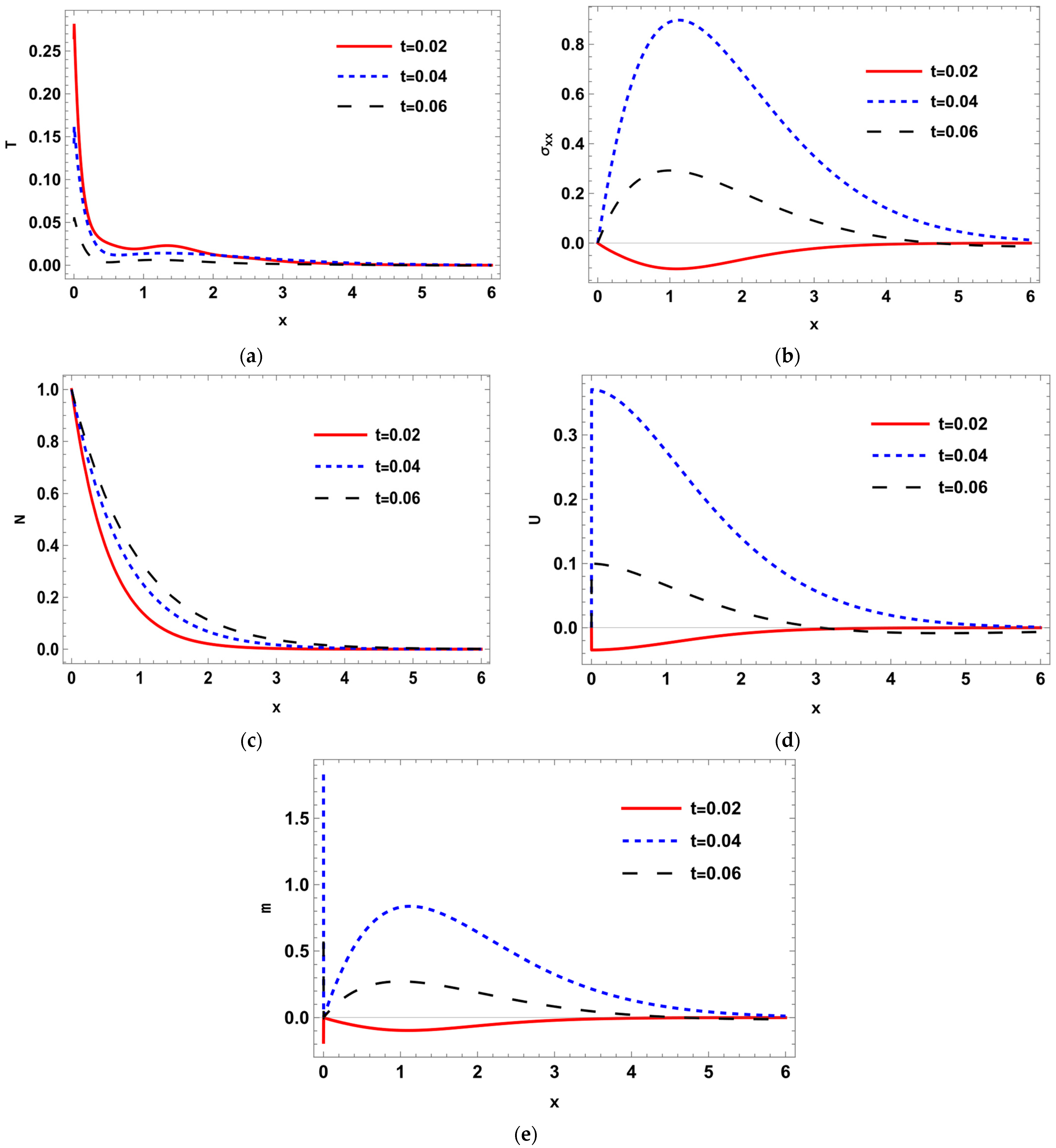
Figure 1. (ae) The deterministic temperature, normal stress, carrier density, displacement, and moisture distributions along the distance for various values of times in relation to generalized photo-thermoelasticity theory.
Crystals 13 00042 g001
Figure 2. (ae) The deterministic and stochastic distributions of temperature, normal stress, carrier density, displacement, and moisture distributions along the distance at t = 0.04 in relation to generalized photo-thermoelasticity theory.
Crystals 13 00042 g002
Figure 3. (ae) The variance of temperature, normal stress, carrier density, displacement, and moisture distributions around its mean at different values of times t = 0.02 , t = 0.04 and t = 0.06 .
Crystals 13 00042 g003
Table 1. Physical constants of Si material.
UnitsSymbolSi
N / m 2 λ 6.4 × 10 10 ,
μ 6.5 × 10 10
kg / m 3 ρ 2330
K T 0 800
s τ 5 × 10 5
m 2 / s D E 2.5 × 10 3
m 3 d n 9 × 10 31
eV E g 1.11
K 1 α t 4.14 × 10 6
Wm 1 K 1 k 150
J / kgK C e 695
m / s s 2
- D T k ρ C e
m 2 % H 2 O / s K D T m 2.1 × 10 7
m 2 s K / % H 2 O D m T 0.648 × 10 6
- m 0 10 %
m 2 s 1 D m 0.35 × 10 2
cm / cm % H 2 o α m 2.68 × 10 3
kg / msM k m 2.2 × 10 8
Disclaimer/Publisher’s Note: The statements, opinions and data contained in all publications are solely those of the individual author(s) and contributor(s) and not of MDPI and/or the editor(s). MDPI and/or the editor(s) disclaim responsibility for any injury to people or property resulting from any ideas, methods, instructions or products referred to in the content.