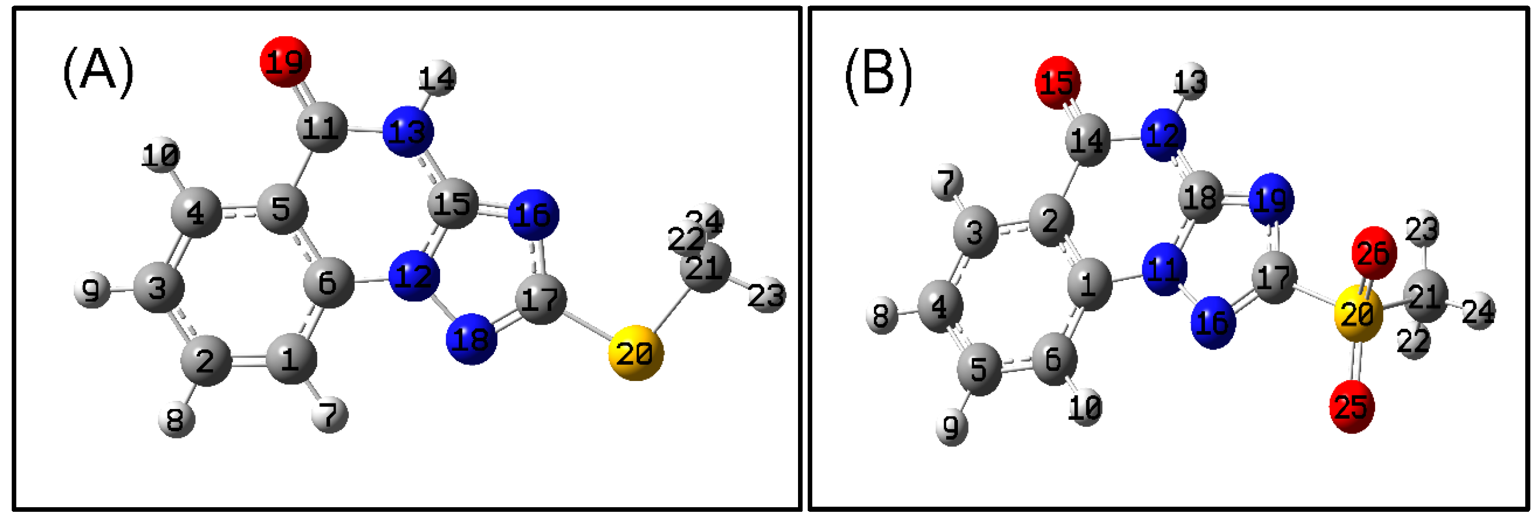
Figure 1.
DIAMOND plots of the asymmetric units for 2-methylthio-triazoloquinazoline (A) and 2-methylsulfonyl-triazoloquinazoline (B) with the atom numbering.
Figure 1.
DIAMOND plots of the asymmetric units for 2-methylthio-triazoloquinazoline (A) and 2-methylsulfonyl-triazoloquinazoline (B) with the atom numbering.
Scheme 1.
Synthetic routes for triazoloquinazolines 1 and 2.
Scheme 1.
Synthetic routes for triazoloquinazolines 1 and 2.
Figure 2.
Depictions of molecular structures for compounds 1 (A,B) and 2 (C,D) using the ωB97XD/6-311G(d,p) theoretical level, presenting both experimental and optimized geometries in a side-by-side comparison. Colored balls represent the atoms, with each color corresponding to a specific element: blue for nitrogen, yellow for sulfur, red for oxygen, the standard element color for carbon, and white for hydrogen.
Figure 3.
Side-by-side presentation of experimental and optimized molecular structures for compounds 1 (A,B) and 2 (C,D), computed using the wB97XD/6-31G(d,p) theoretical approach. Colored balls represent the atoms, with each color corresponding to a specific element: blue for nitrogen, yellow for sulfur, red for oxygen, the standard element color for carbon, and white for hydrogen.
Figure 4.
Partial packing diagram: (A) Depicts compound 1, illustrating the N4–H4…N3 hydrogen bonds represented by blue dashed lines. (B) Showcases compound 2, highlighting the N1–H1…O2 interactions, denoted by red dashed lines. Both diagrams emphasize the relevant hydrogen bonding patterns within each compound.
Figure 5.
Hirshfeld surface analysis of compounds 1 and 2: This figure presents the hirshfeld surface analysis for (A–C) compound 1 and (D–F) compound 2. (A) dnorm visualization for compound 1, with red indicating negative values, white representing zero, and blue signifying positive values. (B) Shape index for compound 1, highlighting the presence of red and blue triangles within the black ellipse, which represent bumps and hollow regions on the shape index surface, respectively. (C) Curvedness analysis for compound 1, identifying planar (green) and curved (blue edge) regions relevant to planar stacking interactions. Similarly, compound 2 is visualized using (D) dnorm, (E) shape index, and (F) curvedness, showcasing the corresponding properties for this compound.
Figure 6.
Hirshfeld surface analysis illustrating intermolecular interactions: This figure depicts the distribution of specific intermolecular interactions for (A) compound 1 and (B) compound 2, as revealed through the Hirshfeld surface analysis. The visual representation of these interactions offers valuable insights into the molecular properties and behavior of both compounds, contributing to their comprehensive characterization and understanding.
Figure 7.
QTAIM Molecular graphs of dimeric models for compound 1: This figure presents two selected dimeric models from the packing structure of compound 1. The atoms are represented by colored balls, with each color corresponding to a specific element: blue for nitrogen, yellow for sulfur, red for oxygen, the standard element color for carbon, and white for hydrogen. The numbers assigned to the atoms range from 1–24 for the first molecule, 25–48 for the second molecule, 49–62 for the third molecule, and 63–86 for the fourth molecule. These visualizations provide valuable insights into the intermolecular interactions and arrangements within the compound’s packing structure.
Figure 8.
QTAIM Molecular graphs of selected trimeric models for compound 2: This figure displays the chosen trimeric models from the packing structure of compound 2. Atoms are represented by colored balls, with each color corresponding to a specific element: blue for nitrogen, yellow for sulfur, red for oxygen, the standard element color for carbon, and white for hydrogen. The atom numbering ranges from 1–26 for the first molecule, 27–52 for the second molecule, and 53–78 for the third molecule. These color-coded and numbered visualizations provide a clear and comprehensive understanding of the molecular structure and composition of compound 2.
Figure 9.
Demonstrating the NCI index as isosurface maps in (B,D), while (A,C) exhibit the RDG scatter plots for compounds 1 and 2, respectively, all determined using the B3LYP-D3/6-311G theoretical framework. Utilizing an RDG boundary of sign(λ2)ρ = 0.5 a.u. and a color scale extending from −0.035 to 0.02 a.u., attractive, van der waals, and repulsive forces are denoted by blue, green, and red surfaces, respectively.
Figure 10.
MESP displays maps for the analyzed triazoloquinazolines 1 (A) and 2 (B) at two distinct sites.
Figure 10.
MESP displays maps for the analyzed triazoloquinazolines 1 (A) and 2 (B) at two distinct sites.
Figure 11.
Ball and stick model of (A) compound 1 and (B) compound 2 visualizing the number of atoms. The ball and stick model provides a 3D representation of the molecular structure where the balls represent atoms and sticks represent chemical bonds. colored balls represent atoms, with each color corresponding to a specific element: blue for nitrogen, yellow for sulfur, red for oxygen, the standard element color for carbon, and white for hydrogen. The numbers assigned to the atoms indicate their positions within the molecular structure.
Table 1.
Crystal data and details of the structure determination [
8,
10].
Table 1.
Crystal data and details of the structure determination [
8,
10].
| Identification Code | Compound 1 | Compound 2 |
|---|
| CCDC | 887013 | 887014 |
| Empirical formula | C10H8N4OS | C10H8N4O3S |
| Formula weight | 232.26 | 264.26 |
| Temperature/K | 294(2) | 294(2) |
| Crystal system | Monoclinic | monoclinic |
| Space group | P21/c | P21 |
| a/Å | 10.41500(10) | 9.6216(2) |
| b/Å | 5.06310(10) | 4.92060(10) |
| c/Å | 18.6564(3) | 12.1623(3) |
| α/° | 90 | 90 |
| β/° | 96.8570(10) | 106.628(2) |
| γ/° | 90 | 90 |
| Volume/Å3 | 976.76(3) | 551.73(2) |
| Z | 4 | 2 |
| ρcalcg/cm3 | 1.579 | 1.591 |
| μ/mm−1 | 2.813 | 2.711 |
| F(000) | 480 | 272 |
| Crystal size/mm3 | 0.35 × 0.15 × 0.1 | 0.2 × 0.1 × 0.02 |
| Radiation | CuKα (λ = 1.54184) | CuKα (λ = 1.54184) |
| 2Θ range for data collection/° | 8.56 to 153.78 | 7.58 to 153.36 |
| Index ranges | −13 ≤ h ≤ 13, −6 ≤ k ≤ 6, −23 ≤ l ≤ 23 | −12 ≤ h ≤ 12, −6 ≤ k ≤ 6, −14 ≤ l ≤ 15 |
| Reflections collected | 15,980 | 9640 |
| Independent reflections | 2052 [Rint = 0.0328, Rsigma = 0.0130] | 2304 [Rint = 0.0247, Rsigma = 0.0176] |
| Data/restraints/parameters | 2052/0/151 | 2304/1/168 |
| Goodness-of-fit on F2 | 1.054 | 1.039 |
| Final R indexes [I >= 2σ (I)] | R1 = 0.0303, wR2 = 0.0883 | R1 = 0.0299, wR2 = 0.0807 |
| Final R indexes [all data] | R1 = 0.0310, wR2 = 0.0894 | R1 = 0.0311, wR2 = 0.0820 |
| Largest diff. peak/hole/e Å−3 | 0.24/−0.21 | 0.15/−0.26 |
Table 2.
Comparison of experimental (X-ray) and theoretical [B3LYP/6-311G(d,p)] lengths (Å) for compounds 1 and 2.
Table 2.
Comparison of experimental (X-ray) and theoretical [B3LYP/6-311G(d,p)] lengths (Å) for compounds 1 and 2.
| Compound 1 | Compound 2 |
|---|
| | Length/Å | | | | Length/Å | | |
|---|
| Atom | SC-XRD | DFT | MAE | MSE | Atom | SC-XRD | DFT | MAE | MSE |
|---|
| S1—C9 | 1.7402(14) | 1.7522 | 0.012 | 0.000144 | S1—O2 | 1.4421(16) | 1.391 | 0.0511 | 0.002611 |
| S1—C10 | 1.7980(15) | 1.814 | 0.016 | 0.000256 | S1—O3 | 1.4296(16) | 1.3927 | 0.0369 | 0.001362 |
| O1—C7 | 1.2145(18) | 1.2131 | 0.0014 | 1.96 × 10⁻⁶ | S1—C9 | 1.7726(17) | 1.723 | 0.0496 | 0.00246 |
| N1—N2 | 1.3848(15) | 1.3678 | 0.017 | 0.000289 | S1—C10 | 1.744(2) | 1.6803 | 0.0637 | 0.004058 |
| N1—C1 | 1.3897(17) | 1.3904 | 0.0007 | 4.90 × 10⁻⁷ | O1—C1 | 1.211(2) | 1.2417 | 0.0307 | 0.000942 |
| N1—C8 | 1.3443(15) | 1.3528 | 0.0085 | 7.22 × 10⁻⁵ | N1—C1 | 1.370(3) | 1.404 | 0.034 | 0.001156 |
| N2—C9 | 1.3237(17) | 1.3188 | 0.0049 | 2.40 × 10⁻⁵ | N1—C8 | 1.364(2) | 1.3869 | 0.0229 | 0.000524 |
| N3—C8 | 1.3192(18) | 1.3109 | 0.0083 | 6.89 × 10⁻⁵ | N2—N3 | 1.3718(19) | 1.3354 | 0.0364 | 0.001325 |
| N3—C9 | 1.3759(16) | 1.3711 | 0.0048 | 2.30 × 10⁻⁵ | N2—C7 | 1.397(2) | 1.4122 | 0.0152 | 0.000231 |
| N4—C7 | 1.3800(19) | 1.3918 | 0.0118 | 0.000139 | N2—C8 | 1.348(2) | 1.4471 | 0.0991 | 0.009821 |
| N4—C8 | 1.3614(17) | 1.3668 | 0.0054 | 2.92 × 10⁻⁵ | N3—C9 | 1.312(2) | 1.3664 | 0.0544 | 0.002959 |
| C1—C2 | 1.3942(17) | 1.3946 | 0.0004 | 1.60 × 10⁻⁷ | N4—C8 | 1.321(2) | 1.3662 | 0.0452 | 0.002043 |
| C1—C6 | 1.4008(18) | 1.4032 | 0.0024 | 5.76 × 10⁻⁶ | N4—C9 | 1.355(2) | 1.4124 | 0.0574 | 0.003295 |
| C2—C3 | 1.378(2) | 1.3868 | 0.0088 | 7.74 × 10⁻⁵ | C1—C2 | 1.479(3) | 1.4802 | 0.0012 | 1.44 × 10⁻⁶ |
| C3—C4 | 1.390(2) | 1.3996 | 0.0096 | 9.22 × 10⁻⁵ | C2—C3 | 1.397(3) | 1.3999 | 0.0029 | 8.41 × 10⁻⁶ |
| C4—C5 | 1.3800(19) | 1.3853 | 0.0053 | 2.81 × 10⁻⁵ | C2—C7 | 1.395(2) | 1.4193 | 0.0243 | 0.00059 |
| C5—C6 | 1.391(2) | 1.3973 | 0.0063 | 3.97 × 10⁻⁵ | C3—C4 | 1.377(3) | 1.3912 | 0.0142 | 0.000202 |
| C6—C7 | 1.4828(18) | 1.4828 | 0 | 0 | C4—C5 | 1.387(3) | 1.3965 | 0.0095 | 9.03 × 10⁻⁵ |
| | 0.006867 | 7.17 × 10⁻⁵ | C5—C6 | 7.17 × 10⁻⁵ | 1.3917 | 0.0127 | 0.000161 |
| | | | | | C6—C7 | 1.385(2) | 1.4081 | 0.0231 | 0.000534 |
| | | | | | | 0.034225 | 0.001719 |
Table 3.
Comparative analysis of experimental (X-ray) and theoretical [B3LYP/6-311G(d,p)] angles (in degrees) for compounds 1 and 2.
Table 3.
Comparative analysis of experimental (X-ray) and theoretical [B3LYP/6-311G(d,p)] angles (in degrees) for compounds 1 and 2.
| Compound 1 | Angle/° | | | Compound 2 | Angle/° | | |
|---|
| Atoms | SC-XRD | DFT | MAE | MSE | Atoms | SC-XRD | DFT | MAE | MSE |
|---|
| C9—S1—C10 | 100.67(7) | 99.4244 | 1.2456 | 1.551519 | O2—S1—C9 | 105.18(9) | 108.6153 | 3.4353 | 11.80129 |
| N2—N1—C1 | 126.72(10) | 127.0981 | 0.3781 | 0.14296 | O2—S1—C10 | 109.57(10) | 110.4953 | 0.9253 | 0.85618 |
| C8—N1—N2 | 109.76(10) | 109.1637 | 0.5963 | 0.355574 | O3—S1—O2 | 119.93(11) | 117.6775 | 2.2525 | 5.073756 |
| C8—N1—C1 | 123.49(11) | 123.7383 | 0.2483 | 0.061653 | O3—S1—C9 | 108.24(9) | 109.1524 | 0.9124 | 0.832474 |
| C9—N2—N1 | 101.13(10) | 101.6318 | 0.5018 | 0.251803 | O3—S1—C10 | 109.44(11) | 109.7427 | 0.3027 | 0.091627 |
| C8—N3—C9 | 102.03(11) | 101.5335 | 0.4965 | 0.246512 | C10—S1—C9 | 103.09(9) | 99.6218 | 3.4682 | 12.02841 |
| C8—N4—C7 | 123.00(11) | 123.6761 | 0.6761 | 0.457111 | C8—N1—C1 | 122.54(16) | 120.7368 | 1.8032 | 3.25153 |
| N1—C1—C2 | 122.47(12) | 122.0837 | 0.3863 | 0.149228 | N3—N2—C7 | 126.61(13) | 129.5362 | 2.9262 | 8.562646 |
| N1—C1—C6 | 116.55(11) | 116.7211 | 0.1711 | 0.029275 | C8—N2—N3 | 109.28(14) | 109.4571 | 0.1771 | 0.031364 |
| C2—C1—C6 | 120.97(12) | 121.1952 | 0.2252 | 0.050715 | C8—N2—C7 | 124.09(14) | 121.0067 | 3.0833 | 9.506739 |
| C3—C2—C1 | 118.83(13) | 118.6206 | 0.2094 | 0.043848 | C9—N3—N2 | 100.69(13) | 105.4517 | 4.7617 | 22.67379 |
| C2—C3—C4 | 121.01(13) | 121.0563 | 0.0463 | 0.002144 | C8—N4—C9 | 100.67(15) | 103.4791 | 2.8091 | 7.891043 |
| C5—C4—C3 | 119.85(13) | 119.8135 | 0.0365 | 0.001332 | O1—C1—N1 | 120.47(19) | 117.9045 | 2.5655 | 6.58179 |
| C4—C5—C6 | 120.60(13) | 120.2804 | 0.3196 | 0.102144 | O1—C1—C2 | 123.5(2) | 124.0836 | 0.5836 | 0.340589 |
| C1—C6—C7 | 121.28(13) | 121.6514 | 0.3714 | 0.137938 | N1—C1—C2 | 116.01(16) | 118.0117 | 2.0017 | 4.006803 |
| C5—C6—C1 | 118.70(12) | 119.0339 | 0.3339 | 0.111489 | C3—C2—C1 | 120.22(17) | 118.8431 | 1.3769 | 1.895854 |
| C5—C6—C7 | 120.00(12) | 119.3147 | 0.6853 | 0.469636 | C7—C2—C1 | 121.66(16) | 121.8593 | 0.1993 | 0.03972 |
| O1—C7—N4 | 121.17(13) | 120.9174 | 0.2526 | 0.063807 | C7—C2—C3 | 118.12(18) | 119.2976 | 1.1776 | 1.386742 |
| O1—C7—C6 | 123.63(14) | 124.4552 | 0.8252 | 0.680955 | C4—C3—C2 | 120.10(18) | 120.3188 | 0.2188 | 0.047873 |
| N4—C7—C6 | 115.18(12) | 114.6274 | 0.5526 | 0.305367 | C3—C4—C5 | 120.47(18) | 120.1428 | 0.3272 | 0.10706 |
| N1—C8—N4 | 120.29(12) | 119.5857 | 0.7043 | 0.496038 | C6—C5—C4 | 120.88(19) | 120.929 | 0.049 | 0.002401 |
| N3—C8—N1 | 111.11(11) | 111.5024 | 0.3924 | 0.153978 | C5—C6—C7 | 118.24(18) | 119.2141 | 0.9741 | 0.948871 |
| N3—C8—N4 | 128.60(11) | 128.9119 | 0.3119 | 0.097282 | C2—C7—N2 | 115.60(15) | 117.3809 | 1.7809 | 3.171605 |
| N2—C9—S1 | 125.39(9) | 123.963 | 1.427 | 2.036329 | C6—C7—N2 | 122.22(16) | 122.5214 | 0.3014 | 0.090842 |
| N2—C9—N3 | 115.95(12) | 116.1686 | 0.2186 | 0.047786 | C6—C7—C2 | 122.18(17) | 120.0977 | 2.0823 | 4.335973 |
| N3—C9—S1 | 118.65(10) | 119.8684 | 1.2184 | 1.484499 | N2—C8—N1 | 119.95(15) | 121.0028 | 1.0528 | 1.108388 |
| | | | 0.493488 | 0.366574 | N4—C8—N1 | 128.56(17) | 130.6879 | 2.1279 | 4.527958 |
| | | | | | N4—C8—N2 | 111.47(16) | 108.3091 | 3.1609 | 9.991289 |
| | | | | | N3—C9—S1 | 121.05(13) | 124.8163 | 3.7663 | 14.18502 |
| | | | | | N3—C9—N4 | 117.88(15) | 113.3029 | 4.5771 | 20.94984 |
| | | | | | N4—C9—S1 | 120.94(13) | 121.8281 | 0.8881 | 0.788722 |
| | | | | | | | | 1.808658 | 5.068006 |
Table 4.
Geometrical measurements associated with various intermolecular and intermolecular interactions (distances in Å and angles in degrees).
Table 4.
Geometrical measurements associated with various intermolecular and intermolecular interactions (distances in Å and angles in degrees).
| Atoms | D–H…A | d(D-H)/Å | d(H-A)/Å | d(D-A)/Å | D-H-A/° | Symmetry Codes |
|---|
| Comp 1 | N4–H4…N3 | 0.85(2) | 2.05(2) | 2.896(2) | 174(2) | X,1-Y,-Z |
| Comp 2 | N1–H1…O2 | 0.880(10) | 2.230(10) | 3.072(2) | 160(3) | 1-X,1/2+Y,-Z |
Table 5.
Chosen energetic characteristics of compound 1 and 2 dimers, determined using the wB97XD method alongside the 6-311G(d,p) basis set.
Table 5.
Chosen energetic characteristics of compound 1 and 2 dimers, determined using the wB97XD method alongside the 6-311G(d,p) basis set.
| Conformation | ∆E
(kcal/mole) | BSSE
(kcal/mole) | ∆E(BSSE)
(kcal/mole) |
|---|
| A | 1.19 | 4.969 | 6.16 |
| B | −5.08 | 1.010 | −4.08 |
| C | −12.05 | 7.097 | −4.96 |
| D | −22.56 | 5.095 | −17.47 |
| E | −4.52 | 1.286 | −3.24 |
| F | −24.63 | 5.993 | −18.64 |
Table 6.
The topological characteristics of chosen non-covalent intermolecular and intramolecular connections at the bond critical point, for compounds 1 and 2 were calculated using the B3LYP/6-311G(d,p) theoretical approach.
Table 6.
The topological characteristics of chosen non-covalent intermolecular and intramolecular connections at the bond critical point, for compounds 1 and 2 were calculated using the B3LYP/6-311G(d,p) theoretical approach.
| | BCP | Atoms | ρ(r) | ∇2ρ(r) | Ellipticity | K | BPL | V | G | |V(r)|/G(r) |
|---|
| Cp. 1 | 2 | N4—H35 | 0.006289 | 0.022212 | 0.113048 | 0.000705 | 5.140017 | −0.00414 | 0.004849 | 0.854609 |
| 26 | C32—O74 | 0.002331 | 0.007681 | 0.373475 | 0.000422 | 8.496853 | −0.00108 | 0.001499 | 0.718479 |
| 28 | H22—O74 | 0.008058 | 0.033277 | 0.112983 | 0.000988 | 4.8339 | −0.00634 | 0.007332 | 0.865248 |
| 35 | N27—C86 | 0.002116 | 0.007772 | 1.994151 | 0.000359 | 7.571653 | −0.00123 | 0.001585 | 0.773502 |
| 37 | C40—C88 | 0.002703 | 0.007564 | 1.070424 | 0.000347 | 7.568092 | −0.0012 | 0.001545 | 0.775405 |
| 58 | H48—S49 | 0.009736 | 0.044927 | 0.042777 | 0.001263 | 5.028214 | −0.00871 | 0.009968 | 0.873295 |
| 61 | N52—H83 | 0.006285 | 0.0222 | 0.11302 | 0.000705 | 5.140599 | −0.00414 | 0.004846 | 0.854519 |
| 63 | N30—C84 | 0.001735 | 0.007364 | 0.982007 | 0.000343 | 7.38067 | −0.00116 | 0.001499 | 0.771181 |
| 84 | O26—C80 | 0.00233 | 0.007679 | 0.373457 | 0.000422 | 8.497276 | −0.00108 | 0.001498 | 0.718291 |
| 85 | O26—H70 | 0.008056 | 0.033269 | 0.113215 | 0.000988 | 4.834342 | −0.00634 | 0.007329 | 0.865193 |
| 91 | C38—N75 | 0.002115 | 0.00777 | 2.007461 | 0.000358 | 7.572067 | −0.00123 | 0.001584 | 0.77399 |
| 95 | S1—H96 | 0.009735 | 0.044921 | 0.042777 | 0.001264 | 5.02833 | −0.0087 | 0.009967 | 0.873181 |
| 96 | C36—N78 | 0.001736 | 0.007364 | 0.980273 | 0.000342 | 7.380474 | −0.00116 | 0.001499 | 0.771848 |
| Cp. 2 | 28 | H26—H43 | 0.00125 | 0.004449 | 1.398681 | 0.000312 | 5.768847 | −0.00049 | 0.0008 | 0.61 |
| 47 | O4—C44 | 0.003221 | 0.012971 | 0.939037 | 0.000607 | 6.92691 | −0.00203 | 0.002637 | 0.769814 |
| 48 | N8—H43 | 0.006246 | 0.024646 | 0.232877 | 0.0012 | 5.249185 | −0.00376 | 0.004962 | 0.758162 |
| 49 | H19—C42 | 0.00253 | 0.007617 | 0.381515 | 0.000456 | 6.695947 | −0.00099 | 0.001448 | 0.685083 |
| 54 | C18—O56 | 0.003229 | 0.012955 | 0.922371 | 0.000601 | 6.906885 | −0.00204 | 0.002637 | 0.772089 |
| 61 | H51—O55 | 0.006083 | 0.028012 | 0.799943 | 0.001387 | 5.645358 | −0.00423 | 0.005616 | 0.753027 |
| 63 | N34—O55 | 0.003969 | 0.016565 | 0.327863 | 0.00065 | 7.549581 | −0.00284 | 0.003492 | 0.81386 |
| 64 | N34—O56 | 0.003614 | 0.016076 | 0.130798 | 0.000491 | 6.45756 | −0.00304 | 0.003528 | 0.860828 |
| 66 | C44—O56 | 0.001118 | 0.006521 | 0.708403 | 0.000421 | 7.459908 | −0.00079 | 0.001209 | 0.651778 |
| 67 | H52—O56 | 0.00249 | 0.013368 | 0.190436 | 0.000822 | 5.731315 | −0.0017 | 0.002521 | 0.673939 |
| 70 | C40—N59 | 0.004426 | 0.012864 | 0.469134 | 0.00035 | 7.335367 | −0.00252 | 0.002867 | 0.877921 |
| 71 | C44—N60 | 0.003265 | 0.010471 | 0.854723 | 0.000425 | 7.250512 | −0.00177 | 0.002192 | 0.806113 |
| 74 | H17—N60 | 0.006257 | 0.024645 | 0.235346 | 0.001199 | 5.250095 | −0.00376 | 0.004962 | 0.758364 |
| 78 | C37—N61 | 0.003655 | 0.010319 | 0.466641 | 0.000393 | 7.100146 | −0.00179 | 0.002187 | 0.820302 |
| 79 | C46—C74 | 0.00326 | 0.009824 | 1.03613 | 0.000481 | 7.154223 | −0.00149 | 0.001974 | 0.756332 |
| 92 | C16—H71 | 0.002573 | 0.007717 | 0.433497 | 0.000461 | 6.787062 | −0.00101 | 0.001469 | 0.686181 |
| 100 | H17—H78 | 0.001246 | 0.004458 | 8.173816 | 0.000309 | 5.807382 | −0.0005 | 0.000805 | 0.616149 |
Table 7.
The global descriptors of the compound 1 and 2.
Table 7.
The global descriptors of the compound 1 and 2.
| Global Descriptors | Compound 1 | Compound 2 |
|---|
| E_HOMO(N) (eV) | −6.0688 | −7.2636 |
| E_HOMO(N+1) (eV) | 1.7367 | 1.2328 |
| E_HOMO(N−1) (eV) | −10.9226 | −11.8528 |
| Vertical (IP) (eV) | 7.7485 | 8.894 |
| Vertical (EA) (eV) | 0.0255 | 0.4702 |
| Mulliken electronegativity (eV) | 3.887 | 4.6821 |
| Chemical potential (μ) (eV) | −3.887 | −4.6821 |
| Hardness (η) (eV) | 7.723 | 8.4238 |
| Softness (S) (eV−1) | 0.1295 | 0.1187 |
| Electrophilicity index (ω) (eV) | 0.9782 | 1.3012 |
| Nucleophilicity index (N) (eV) | 3.0524 | 1.8576 |
Table 8.
Local electrophilic P+ and nucleophilic P− Parr functions computed with Mulliken atomic spin densities for compounds 1 and 2 (all results in kJ/mol).
Table 8.
Local electrophilic P+ and nucleophilic P− Parr functions computed with Mulliken atomic spin densities for compounds 1 and 2 (all results in kJ/mol).
| Compound 2 | Compound 1 |
|---|
| Atoms | P− | P+ | f0 | Atoms | (P+) | (P−) | f0 |
|---|
| C1 | 447.28 | 166.77 | 121.56 | C1 | 195.43 | −7.35 | 124.45 |
| C2 | 476.92 | 181.24 | 122.09 | C2 | −116.57 | 938.72 | 185.1 |
| C3 | 340.39 | −30.09 | 133.11 | C3 | 304.5 | −291.51 | 134.16 |
| C4 | −97.8 | 556.11 | 174.86 | C4 | −57.1 | 684.78 | 142.83 |
| C5 | 849.93 | −176.33 | 185.89 | C5 | 151.19 | 318.02 | 103.44 |
| C6 | −254.2 | 280.53 | 122.35 | C6 | −7.61 | 223.25 | 74.56 |
| H7 | −21.58 | 0.21 | 77.45 | H7 | −10.66 | −5.99 | 68 |
| H8 | 0.62 | −28.07 | 95.83 | H8 | 4.59 | −61.33 | 97.93 |
| H9 | −55.9 | 6.59 | 102.92 | H9 | −14.83 | 12.15 | 82.97 |
| H10 | 9.14 | −15.88 | 72.2 | H10 | 1.98 | −41.27 | 76.93 |
| N11 | −65.61 | 438.06 | 68 | C11 | −69.6 | 447.77 | 142.04 |
| N12 | 137.13 | 275.75 | 112.63 | N12 | 348.88 | 22.13 | 68.26 |
| H13 | −9.45 | −12.42 | 78.77 | N13 | 114.53 | 72.15 | 85.85 |
| C14 | 342.34 | −136.03 | 136.79 | H14 | −5.93 | −9.01 | 68.53 |
| O15 | 289.44 | 388.28 | 249.95 | C15 | 90.49 | −7.12 | 64.59 |
| N16 | 39.92 | 114.61 | 99.51 | N16 | −52.4 | −1.76 | 85.85 |
| C17 | 145.22 | 348.13 | 123.14 | C17 | 23.91 | −0.26 | 78.5 |
| C18 | 35.67 | 175.46 | 71.68 | N18 | 430.67 | −3.02 | 116.83 |
| N19 | −26.23 | −117.04 | 103.44 | O19 | 211.64 | 335.37 | 227.63 |
| S20 | 25.01 | −56.16 | 50.41 | S20 | 1049.34 | −0.19 | 389.1 |
| C21 | 1.84 | −3.44 | 34.13 | C21 | −43.53 | 0.01 | 56.71 |
| H22 | 0.03 | −0.29 | 22.05 | H22 | 38.47 | −0.01 | 47 |
| H23 | −0.2 | 0.96 | 18.9 | H23 | −0.37 | −0.02 | 57.24 |
| H24 | 6.16 | 2.31 | 49.62 | H24 | 38.47 | −0.01 | 47 |
| O25 | 3.48 | 102.09 | 89.53 | | | | |
| O26 | 5.93 | 164.14 | 108.96 | | | | |
Table 9.
Presents the O–H bond dissociation enthalpy (BDE) values obtained using the B3LYP/6-311G(d,p) method, expressed in kJ/mol.
Table 9.
Presents the O–H bond dissociation enthalpy (BDE) values obtained using the B3LYP/6-311G(d,p) method, expressed in kJ/mol.
| H Atoms | HAT | SET-PT | SPLET |
|---|
| BDE | IP | PDE | PA | ETE |
|---|
| Cp. 1 | Cp. 2 | Cp. 1 | Cp. 2 | Cp. 1 | Cp. 2 | Cp. 1 | Cp. 2 | Cp. 1 | Cp. 2 |
|---|
| H-7 | 482.57 | 481.37 | 734.82 | 853.66 | 1063.64 | 943.61 | 1609.3 | 1597.83 | 189.16 | 199.44 |
| H-8 | 470.52 | 474.35 | 734.82 | 853.66 | 1051.6 | 936.59 | 1618.94 | 1603.12 | 167.48 | 187.12 |
| H-9 | 473.75 | 472.06 | 734.82 | 853.66 | 1054.82 | 934.3 | 1630.51 | 1594.98 | 159.14 | 192.98 |
| H-10 | 480.28 | 483.89 | 734.82 | 853.66 | 1061.36 | 946.13 | 1627.06 | 1577.74 | 169.12 | 222.05 |


