
Formation of Tesseract Time Crystals on a Quantum Computer

Elmore Family School of Electrical and Computer Engineering, Purdue University, West Lafayette, IN 47907, USA
Crystals 2023, 13(8), 1265; https://doi.org/10.3390/cryst13081265
Submission received: 4 July 2023
/
Revised: 10 August 2023
/
Accepted: 13 August 2023
/
Published: 17 August 2023
(This article belongs to the Section Crystal Engineering)
Abstract
:The engineering of new states of matter through Floquet driving has revolutionized the field of condensed matter physics. This technique enables the creation of hybrid topological states and ordered phases that are absent in normal systems. Crystalline structures, exemplifying spatially ordered systems under periodic driving, have been extensively studied. However, recent focus has shifted towards discrete time crystals (DTCs), periodically driven quantum many-body systems that break time translation symmetry under specific conditions. In this paper, the model of discrete time crystals is extended to allow for the formation of time-varying tesseracts, allowing for the investigation of time translational symmetry in pseudo-higher-dimensional lattice systems.
1. Introduction
The engineering of new states of matter using Floquet driving has revolutionized the field of condensed matter physics [1,2,3,4]. By employing this technique, researchers have successfully created hybrid topological states and ordered phases in time that were previously unattainable; while periodic driving of crystalline structures has been extensively investigated, the emergence of discrete time crystals (DTCs) has opened up new avenues for exploration [5]. Unlike their spatial counterparts, DTCs exhibit periodicity in discrete time steps rather than in spatial dimensions. The theoretical foundation of DTCs is rooted in the concept of periodically driven quantum many-body systems that break time translation symmetry [6,7,8,9,10,11,12]. These theoretical predictions have led to the identification of distinctive phases, including the strongly disordered thermal phase and the many-body localization phase [13,14].
Discrete time crystals have been observed in a lattice of interaction spin chains in trapped atomic systems consisting of Yb ions periodically driven by laser pulses [15], and of a chain of trapped P atoms [16]. Time crystals have also been discovered in diamond samples with NV center clusters that are periodically driven with a laser [17]. Recent experimental work has shown that 2D time crystals can be realized with photonic time crystals that are formed on the surface of dialectic substrate FR4 [18]. Continuous time crystals have been realized in 1D [19] and 2D in a Bose–Eisenstein condensate driven by a continuous optical pump [14]. In charge density wave (CDW) materials, such as 1T-TaS, are thin films so that there is little bulk dissipation. Time crystals evolve from electrical driving [20], laser pulses [21], and magnetic field driving [22]. Theoretical models suggest that light or ultrafast charge transfer creates CDW melting, which allows for the material to behave like a time crystal under periodic driving [2,23]. The Ising model, which is the backbone of time crystals, has also been shown to be able to accurately model spin-glass dynamics under certain conditions [24,25]. The DTC phase is also referred to a the spin-glass phase since it forms when all of the flip terms of the Ising Hamiltonian are or 180 [26].
The exploration of DTCs has extended beyond one-dimensional systems, captivating the interest of researchers in higher-dimensional lattice structures [27]. These higher-dimensional systems offer additional degrees of freedom for studying time translational symmetry and the occurrence of multiple distinct phases within a single system [27]. Recent experimental breakthroughs have observed the formation of two spatial dimensional discrete time crystals in crystal systems, shedding light on the dynamics and properties of DTCs in higher dimensions [20,21,23]. It has been shown that when DTCs are extended to higher dimensions, they become more resilient to noise and thermal disorder [28,29].
Quantum computers have emerged as powerful tools for studying and manipulating DTCs. These cutting-edge machines enable the simulation of complex quantum systems, facilitating investigations into the behavior of DTCs in larger systems. Quantum computers also provide insights into the role of quantum entanglement and allow for the exploration of various parameters and driving protocols that influence the stability and properties of DTCs. Furthermore, the unique control capabilities of quantum computers make it possible to design optimal driving protocols for creating and sustaining DTCs [26,30]. Advanced control techniques, such as optimal control theory and machine learning algorithms, can be employed to devise robust time evolution protocols. Recently, it has been shown that higher-dimensional time crystals can be formed on a quantum computer by taking advantage of hardware connectivity [31].
To progress the understanding of time translational symmetry within the context of higher-dimensional systems, a novel concept is proposed: the creation of tesseracts using discrete time crystals. A tesseract serves as a four-dimensional analog of a cube, and its construction via DTCs is an exciting development for understanding higher-dimensional systems. Understanding the formation of tesseracts provides a platform to investigate the intricate interactions between time translational symmetry and the dynamics of higher dimensions. In addition, it provides vital insights into the stability, robustness, and emergent phenomena related to DTCs in systems where dimensions [28,29].
This work presents the study of forming temporal tesseracts on a quantum computer by capitalizing on orthogonal rotations and many-body localization (MBL) interactions by leveraging quantum algorithms. It is noteworthy that this research shows it is feasible to construct objects of dimensions beyond 2D on a quantum computer, thanks to the exploitation of both time and spatial translational symmetries.
2. Discrete Time Crystals
A 1D DTC can be described as a many-body Bloch–Floquet Hamiltonian with phase flip and disorder terms [32,33,34,35,36].
One Bloch–Floquet cycle is defined as H, which consists of , , and . () is the driving phase, where the system is driven by an external force that is scaled by g, the Rabi frequency (0 to 1), and a small perturbation factor, , for fine tuning. The Pauli matrix (e.g., ) determines which axis the driving for is along. () is the coupling Hamiltonian that represents the Ising coupling, where spin i and j of the system interact in a manner that couples them together. In this simulation, a two-qubit gate is used in order to simulate the interaction between two quantum spins. The Ising coupling can be scaled from to and is symmetric about 0 in this system. is the disorder Hamiltonian where spins are rotated by the onsite disorder term, (0 to ). The Pauli matrices in Equation (1) are used to define which axis the Hamiltonians are coupled to () [37,38,39,40,41,42].
In order to form DTCs on a quantum computer, a separate algorithm needs to be implemented; the following shows the Floquet unitary for a 1D DTC system:
where the gate angles are (), , and ; the final wave function is ; and is the initial state. While this unitary is an example, any orthogonal set of gates can be defined and utilized to form a DTC on a quantum computer.
3. A 4D Discrete Time Crystal
Previous works cover the formation of a 1D and a 2D discrete time crystal on a quantum computer. However, in order to extend this to higher time dimensions, the orthogonal rotations need to be taken advantage of for a pseudo-4D-rotation matrix. The 4D point system can be defined with two spatial components and two orthogonal driving components, . Since X and Y correspond to the qubit locations on a quantum computer, only two orthogonal qubit rotations are needed to simulate a third and fourth axis. As long as the rotations are orthogonal, it is possible to construct a pseudo-rotation about an axis for a 4D object.
For the 4D DTC modeled with the Cirq quantum simulator for 50 Floquet time steps with 16 qubits, and are the terms chosen because they are the only terms that lead to a symmetric rotation about the fourth axis. This is because all rotations that are in the quantum system must be isometric, as opposed to the true rotation matrix, which allows for any arbitrary rotation where the relation between all points is conserved. In order to model a hypercube, 16 qubits are utilized. More qubits can be added to the model to simulate higher node count objects (Figure A1). In addition, more Ising interactions can be added to simulate more edges in order to model different objects.
When the qubits are rotated with the phased X gate and the interaction term is orthogonal to the ZZ gate, it is possible to realize a 4D object with a rotation about the fourth axis. This corresponds to a rotation of a tesseract in 4D. This rotation means that a plane in 2D is crossed every four iterations, which corresponds to a total rotation of . In order for the system to rotate to its initial state, a total of 24 rotations is required. The system starts out with the initial state (Figure 1A). The first iteration rotates all qubits to the X axis. In the absence of the interaction term, the next rotation will bring all qubits to the |1〉 state. However, with the ZZ interaction term, only the qubits on the corners and are in the |1〉 state. After a total of four time steps, , , , and qubits become fully polarized, and these qubits correspond to the inner 4 qubits of a 16-qubit square. This corresponds to a 2D intersection of a 4D tesseract and a 2D plane. This shows that the interaction terms create a higher-dimensional object with pseudo-rotations about a higher-dimensional axis. This inner box corresponds to the “inner box” of the hypercube that is a tesseract. All even interactions do not intersect a higher-dimensional plane and, thus, do not show any states on the computational basis. The third iteration shows that a box has formed inside the 2D qubit grid (, , , and ). This inner box corresponds to the “inner box” of the hypercube that is a tesseract. After four rotations, the other side of the inner cube appears in the 2D qubit grid. After another set of rotations, the outer cube plane shows as a fully |1〉-filled qubit grid. This corresponds to the rotational state where both the inner cube and the outer cube exist on the same 2D plane. This process repeats throughout the unitary gates, which shows that this is indeed a 4D hypercube that has formed in a quantum circuit (Figure 1A). The corner modes in qubits 4 and 13 arise due to edge interactions from the discrete edge that forms due to algorithm limitations; since there will always be a leading and trailing qubit, this will appear in the algorithm and in real experiments. Figure 1 shows the unitary with different sets of orthogonal rotation gates. Figure 1B: rotation in Y and interaction terms in ZZ. Figure 1C: rotation in X and interaction terms in YY. Figure 1D: rotation in Y and interaction terms in XX.
The 4D discrete time crystal is an expanded form of the 2D discrete time crystal. The first part of the state is the qubits being arranged in a “virtual” 2D spatial crystal, which corresponds to the 2D grid layout of the quantum computer. The third and fourth axis are formed from the rotation gates being forced to be orthogonal, and the disorder term is eliminated from the unitary. By leveraging both of these components, it is possible to form a 4D crystal state.
In order to demonstrate the 2D nature of the qubits and their time evolution, the qubit structure is rearranged into a 2D grid, and time evolution is applied to the unitary operations. By arranging the qubits in a 2D formation, it is easier to see the 4D rotations with a 2D projection, , where corresponds to projection onto a 2D axis (Figure 2). In order to skip the blank states, only every other time step is taken into account. The edge states appear due to the NN algorithm needing to have start and end points; this leads to there being a dangling edge state in the 2D lattice.
The projection of a hypercube onto a 2D project can be described as a hypercube graph, where the graph is defined as and n is the dimension of the graph. A cube graph () has 8 vertices and 12 edges, which corresponds to a three-dimensional cube. There are vertices and edges. A graph is a Levi graph in the Mobius configuration that describes a higher-dimensional tetrahedron in Euclidean or projective space. In the hypercube graph, each vertex of the hypercube is labeled, and its connectivity is described by the edges of the graph. The adjacency matrix of this graph can be seen as equivalent to the 2D projection matrix represented by a 2D lattice of 16 connected qubits for a hyper-dimensional cube .
4. Prethermal Phase
4.1. Thermalization
In order to demonstrate the evolution from the thermal (noisy) phase to the more ordered many-body localization phase, a model that consists of a phased XZ gate and a stable Ising interaction gate, ZZ(), is constructed. The onsite disorder from long-range interactions () is set to 0, and the coupling parameter (g) is set to 1. In order to vary the phase flip, the fine-tuning parameter () is varied. Under small driving (), the system stays in an energetically low state with the majority of states being |0〉 (Figure 3A). The dephasing in qubits 13 and 4 is due to edge effects in the system. As is decreased to 0.9, the system begins to take on a more ordered state with a time-evolved state on and (Figure 3B). When is further decreased to 0.75, the driving force becomes ; this increases the frequency of the periodic state on and , while the rest of the system remains in a thermal state (Figure 3C). Upon reaching , the system enters a critical point where the driving force has a frequency of . The driving force is now equal to the Ising interaction, ZZ, even in the “low” driving state where the system should still be in the thermal state (thermal states exist for g < 0.9); the system becomes strongly correlated and forms tesseract-like states (Figure 3D). Decreasing further shows a mirror of the previous observations.
4.2. Onsite Disorder
By setting g = 5, the onsite disorder can be tuned independently to see the effects of local fields on the system in the MBL phase. First, a small amount of disorder is added to the system ( = 0.01). The MBL form is strong in the first 10 time steps; however, there is an increasing amount of disorder in the system, and eventually, it will completely dephase (Figure 4A). After increasing the onsite disorder to 0.1, the system becomes completely dephased with no recovery of the MBL state (Figure 4B). This shows that the MBL state is extremely fragile to onsite disorder in the system. It is important to note that = 0.1 is a large amount of disorder to input into a quantum system where the maximum amount of onsite potential that can be added is = 1. Similar results can be seen when the disorder term is increased to 0.25 (Figure 4C). Upon reaching = 0.5, the system reaches a new critical point where it becomes stabilized from the onsite disorder. This is due to being 100% in phase with the driving forces of the system (Figure 4D).
5. Discussion
Higher-spatial-dimension time crystals have more connectivity than 1D time crystals. The Ising interaction, , increased the interaction terms for the coupling between two qubits. The Ising interaction terms can be considered as an “edge” to a higher-dimensional object, and qubits correspond to edges with their own respective phases. This representation can be utilized as a graph representation of a mathematical object. Hypercubes, or tesseracts, have eight-edge connectivity for each vertex; however, sometimes the edges are aligned and only show four-edge connectivity. By providing eight interaction terms on a 2D lattice and two time-orthogonal rotations, a 2D projection of a 4D time-dimensional (2D + 2) object is formed. With this, a 16-vertex (qubit) object forms a tesseract in the discrete-time crystal system. Such an object can be used as timing on a quantum computer or as a way to control novel algorithms on a quantum computer.
6. Methods
6.1. Simulation
All calculations were performed in Python v3.9.1 with the Google quantum AI Cirq package v1.0.0. GPU acceleration was enabled with the Nvidia cuQuantum 22.07.1 SDK [43]. Qubits were simulated with a grid layout similar to Google quantum machines. All qubits are typically measured on a basis in a quantum machine. However, for this simulation, qubits were measured using CIRQ’s vector-state simulator, and the polarization measurement was then conducted on a basis in order to obtain the qubit rotation with respect to the axis. When mentioned in the text, the qubits were also measured on a basis. The resulting measurement was then extracted with an autocorrelator. The code used in the simulation is available on GitHub: https://github.com/ChristopherSims/Tesseract_TimeCrystal (accessed on 3 July 2023).
6.2. Edge State
When computing the average of the qubit states, all qubits are taken into consideration. Edge qubits and their effects are considered to be part of the system and are integral to the results. The first qubit and the last qubit to be sequenced will always have “dangling” (missing) Ising interactions that will promote edge states in those qubits.
6.3. Circuits
The time crystal algorithm comprises three main stages: rotations, Ising coupling, and long-range interactions (also called onsite disorder; ), denoted as , , and , respectively, (as shown in Equation (1)). Translating the Bloch–Floquet time step into a quantum algorithm involves three simple gates (Figure 5) [31]. The first stage involves single-gate rotations, specifically, gates. In this work, all gates are rotated by as this is the most stable and optimal rotation for a real quantum algorithm. The next stage involves the Ising “spin” interactions, which can be ideally modeled using a two-qubit gate. Although the more generalized FSIM gates have been utilized in previous works to fine tune the circuit, this work focuses on the variation. To form a two-dimensional state, the gates are applied to the nearest neighbors (NNs), with qubits arranged in a theoretical square pattern. Since Google quantum computers are arranged in a square pattern, this algorithm can be effectively implemented using an NN algorithm. Equation (1) utilizes example terms = and = .
In this work, the phased ZZ gate is defined as follows:
This two-qubit gate can be replaced with the two-qubit gates for the other orthogonal axis (XX,YY).
7. Conclusions
In conclusion, by leveraging the Ising model in a quantum machine, a discrete time crystal is able to simulate tesseracts in a quantum computer by utilizing a 2D grid of qubits with orthogonal spin rotations. This work shows that it is possible to construct -dimensional time crystals by leveraging orthogonal rotations with periodic driving of a many-body system. In addition, this work demonstrates the first experimental realization of a higher-dimensional mathematical object. Additionally, by constructing graph models of hyperdimensional objects, it is possible to realize objects like tesseracts experimentally. In future work, gates can be constructed in the unitary so that new pseudo-planes can be constructed in qubit space and new orthogonal rotations can be added to a higher-dimensional spatial and temporal time crystal (e.g., q = ). Finally, this work demonstrates that by developing new models on a quantum computer with different interactions and driving strengths, it is possible to simulate condensed matter effects like spin glass, anti-ferromagnetism, charge-density waves, etc., from a simple Ising model. By continuously developing new interactions beyond what is presented in this work, a better understanding of many-body interactions can be developed from a simple model.
Funding
This research received no external funding.
Data Availability Statement
Code used in this work is publicly available under the GNU GPL v3 license on Github: (https://github.com/ChristopherSims/Tesseract_TimeCrystal) (accessed on 3 July 2023).
Acknowledgments
C.S. acknowledges the generous support from the GEM Fellowship and the Purdue Engineering ASIRE Fellowship.
Conflicts of Interest
The author declares no conflict of interest.
Appendix A
Figure A1.
The 25 node system. The polarization measurement, = , of each qubit for each time step, t, in the system, with for the ZZ interactions, X flips g = 1, = 0, and 8 connectivity. Red, |1〉; blue, |0〉.
Figure A1.
The 25 node system. The polarization measurement, = , of each qubit for each time step, t, in the system, with for the ZZ interactions, X flips g = 1, = 0, and 8 connectivity. Red, |1〉; blue, |0〉.
References
- Wang, Y.H.; Steinberg, H.; Jarillo-Herrero, P.; Gedik, N. Observation of Floquet-Bloch States on the Surface of a Topological Insulator. Science 2013, 342, 453–457. [Google Scholar] [CrossRef] [PubMed]
- Bukov, M.; D’Alessio, L.; Polkovnikov, A. Universal high-frequency behavior of periodically driven systems: From dynamical stabilization to Floquet engineering. Adv. Phys. 2015, 64, 139–226. [Google Scholar] [CrossRef]
- Harper, F.; Roy, R.; Rudner, M.S.; Sondhi, S. Topology and Broken Symmetry in Floquet Systems. Annu. Rev. Condens. Matter Phys. 2020, 11, 345–368. [Google Scholar] [CrossRef]
- Titum, P.; Berg, E.; Rudner, M.S.; Refael, G.; Lindner, N.H. Anomalous Floquet-Anderson Insulator as a Nonadiabatic Quantized Charge Pump. Phys. Rev. X 2016, 6, 021013. [Google Scholar] [CrossRef]
- Gómez-León, A.; Platero, G. Floquet-Bloch Theory and Topology in Periodically Driven Lattices. Phys. Rev. Lett. 2013, 110, 200403. [Google Scholar] [CrossRef]
- Else, D.V.; Bauer, B.; Nayak, C. Floquet Time Crystals. Phys. Rev. Lett. 2016, 117, 090402. [Google Scholar] [CrossRef]
- von Keyserlingk, C.W.; Khemani, V.; Sondhi, S.L. Absolute stability and spatiotemporal long-range order in Floquet systems. Phys. Rev. B 2016, 94, 085112. [Google Scholar] [CrossRef]
- Sacha, K.; Zakrzewski, J. Time crystals: A review. Rep. Prog. Phys. 2017, 81, 016401. [Google Scholar] [CrossRef]
- Wilczek, F. Quantum Time Crystals. Phys. Rev. Lett. 2012, 109, 160401. [Google Scholar] [CrossRef]
- Watanabe, H.; Oshikawa, M. Absence of Quantum Time Crystals. Phys. Rev. Lett. 2015, 114, 251603. [Google Scholar] [CrossRef]
- Huse, D.A.; Nandkishore, R.; Oganesyan, V.; Pal, A.; Sondhi, S.L. Localization-protected quantum order. Phys. Rev. B 2013, 88, 014206. [Google Scholar] [CrossRef]
- Pekker, D.; Refael, G.; Altman, E.; Demler, E.; Oganesyan, V. Hilbert-Glass Transition: New Universality of Temperature-Tuned Many-Body Dynamical Quantum Criticality. Phys. Rev. X 2014, 4, 011052. [Google Scholar] [CrossRef]
- Ge, R.C.; Koshkaki, S.R.; Kolodrubetz, M.H. Cavity induced many-body localization. arXiv 2022, arXiv:2208.06898. [Google Scholar]
- Koshkaki, S.R.; Kolodrubetz, M.H. Inverted many-body mobility edge in a central qudit problem. Phys. Rev. B 2022, 105, l060303. [Google Scholar] [CrossRef]
- Zhang, J.; Hess, P.W.; Kyprianidis, A.; Becker, P.; Lee, A.; Smith, J.; Pagano, G.; Potirniche, I.D.; Potter, A.C.; Vishwanath, A.; et al. Observation of a discrete time crystal. Nature 2017, 543, 217–220. [Google Scholar] [CrossRef]
- Choi, S.; Choi, J.; Landig, R.; Kucsko, G.; Zhou, H.; Isoya, J.; Jelezko, F.; Onoda, S.; Sumiya, H.; Khemani, V.; et al. Observation of discrete time-crystalline order in a disordered dipolar many-body system. Nature 2017, 543, 221–225. [Google Scholar] [CrossRef]
- Rovny, J.; Blum, R.L.; Barrett, S.E. Observation of Discrete-Time-Crystal Signatures in an Ordered Dipolar Many-Body System. Phys. Rev. Lett. 2018, 120, 180603. [Google Scholar] [CrossRef]
- Wang, X.; Mirmoosa, M.S.; Asadchy, V.S.; Rockstuhl, C.; Fan, S.; Tretyakov, S.A. Metasurface-based realization of photonic time crystals. Sci. Adv. 2023, 9, eadg7541. [Google Scholar] [CrossRef]
- Kongkhambut, P.; Skulte, J.; Mathey, L.; Cosme, J.G.; Hemmerich, A.; Keßler, H. Observation of a continuous time crystal. Science 2022, 377, 670–673. [Google Scholar] [CrossRef]
- Yoshida, M.; Suzuki, R.; Zhang, Y.; Nakano, M.; Iwasa, Y. Memristive phase switching in two-dimensional 1T-TaS crystals. Sci. Adv. 2015, 1, e1500606. [Google Scholar] [CrossRef]
- Gao, F.Y.; Zhang, Z.; Sun, Z.; Ye, L.; Cheng, Y.H.; Liu, Z.J.; Checkelsky, J.G.; Baldini, E.; Nelson, K.A. Snapshots of a light-induced metastable hidden phase driven by the collapse of charge order. Sci. Adv. 2022, 8, eabp9076. [Google Scholar] [CrossRef] [PubMed]
- Hu, Y.; Zhang, T.; Zhao, D.; Chen, C.; Ding, S.; Yang, W.; Wang, X.; Li, C.; Wang, H.; Feng, D.; et al. Real-space observation of incommensurate spin density wave and coexisting charge density wave on Cr (001) surface. Nat. Commun. 2022, 13, 445. [Google Scholar] [CrossRef]
- Lee, J.; Bang, J.; Kang, J. Nonequilibrium Charge-Density-Wave Melting in 1T-TaS Triggered by Electronic Excitation: A Real-Time Time-Dependent Density Functional Theory Study. J. Phys. Chem. Lett. 2022, 13, 5711–5718. [Google Scholar] [CrossRef] [PubMed]
- Heim, B.; Rønnow, T.F.; Isakov, S.V.; Troyer, M. Quantum versus classical annealing of Ising spin glasses. Science 2015, 348, 215–217. [Google Scholar] [CrossRef]
- Schmitt, M.; Rams, M.M.; Dziarmaga, J.; Heyl, M.; Zurek, W.H. Quantum phase transition dynamics in the two-dimensional transverse-field Ising model. Sci. Adv. 2022, 8, eabl6850. [Google Scholar] [CrossRef]
- Mi, X.; Ippoliti, M.; Quintana, C.; Greene, A.; Chen, Z.; Gross, J.; Arute, F.; Arya, K.; Atalaya, J.; Babbush, R.; et al. Time-crystalline eigenstate order on a quantum processor. Nature 2021, 601, 531–536. [Google Scholar] [CrossRef]
- Kuroś, A.; Mukherjee, R.; Mintert, F.; Sacha, K. Controlled preparation of phases in two-dimensional time crystals. Phys. Rev. Res. 2021, 3, 043203. [Google Scholar] [CrossRef]
- Pizzi, A.; Nunnenkamp, A.; Knolle, J. Classical Prethermal Phases of Matter. Phys. Rev. Lett. 2021, 127, 140602. [Google Scholar] [CrossRef]
- Pizzi, A.; Nunnenkamp, A.; Knolle, J. Classical approaches to prethermal discrete time crystals in one, two, and three dimensions. Phys. Rev. B 2021, 104, 094308. [Google Scholar] [CrossRef]
- Frey, P.; Rachel, S. Realization of a discrete time crystal on 57 qubits of a quantum computer. Sci. Adv. 2022, 8, eabm7652. [Google Scholar] [CrossRef]
- Sims, C. Simulation of Higher-Dimensional Discrete Time Crystals on a Quantum Computer. Crystals 2023, 13, 1188. [Google Scholar] [CrossRef]
- Nandkishore, R.; Huse, D.A. Many-Body Localization and Thermalization in Quantum Statistical Mechanics. Annu. Rev. Condens. Matter Phys. 2015, 6, 15–38. [Google Scholar] [CrossRef]
- Abanin, D.A.; Altman, E.; Bloch, I.; Serbyn, M. Colloquium: Many-body localization, thermalization, and entanglement. Rev. Mod. Phys. 2019, 91, 021001. [Google Scholar] [CrossRef]
- Ponte, P.; Papić, Z.; Huveneers, F.; Abanin, D.A. Many-Body Localization in Periodically Driven Systems. Phys. Rev. Lett. 2015, 114, 140401. [Google Scholar] [CrossRef]
- Lazarides, A.; Das, A.; Moessner, R. Fate of Many-Body Localization Under Periodic Driving. Phys. Rev. Lett. 2015, 115, 030402. [Google Scholar] [CrossRef]
- Bordia, P.; Lüschen, H.; Schneider, U.; Knap, M.; Bloch, I. Periodically driving a many-body localized quantum system. Nat. Phys. 2017, 13, 460–464. [Google Scholar] [CrossRef]
- Throckmorton, R.E.; Sarma, S.D. Studying many-body localization in exchange-coupled electron spin qubits using spin–spin correlations. Phys. Rev. B 2021, 103, 165431. [Google Scholar] [CrossRef]
- Alet, F.; Laflorencie, N. Many-body localization: An introduction and selected topics. C. R. Phys. 2018, 19, 498–525. [Google Scholar] [CrossRef]
- Chen, C.; Chen, Y.; Wang, X. Many-body localization in the infinite-interaction limit and the discontinuous eigenstate phase transition. NPJ Quantum Inf. 2022, 8, 142. [Google Scholar] [CrossRef]
- Hu, T.; Xue, K.; Li, X.; Zhang, Y.; Ren, H. Excited-state fidelity as a signal for the many-body localization transition in a disordered Ising chain. Sci. Rep. 2017, 7, 577. [Google Scholar] [CrossRef] [PubMed]
- Kjäll, J.A.; Bardarson, J.H.; Pollmann, F. Many-Body Localization in a Disordered Quantum Ising Chain. Phys. Rev. Lett. 2014, 113, 107204. [Google Scholar] [CrossRef] [PubMed]
- Hauke, P.; Heyl, M. Many-body localization and quantum ergodicity in disordered long-range Ising models. Phys. Rev. B 2015, 92, 134204. [Google Scholar] [CrossRef]
- Bayraktar, H.; Charara, A.; Clark, D.; Cohen, S.; Costa, T.; Fang, Y.L.L.; Gao, Y.; Guan, J.; Gunnels, J.; Haidar, A.; et al. cuQuantum SDK: A High-Performance Library for Accelerating Quantum Science. arXiv 2023, arXiv:2308.01999. [Google Scholar]
Figure 1.
Polarization measurement. The polarization measurement, = , of each qubit for each time step, t, in the DTC state, with and . (A) Rotation in X and interaction in ZZ. (B) Rotation in Y and interaction in ZZ. (C) Rotation in X and interaction in YY. (D) Rotation in Y and interaction in XX. All measurements are made on the basis. Red, |1〉; blue, |0〉.
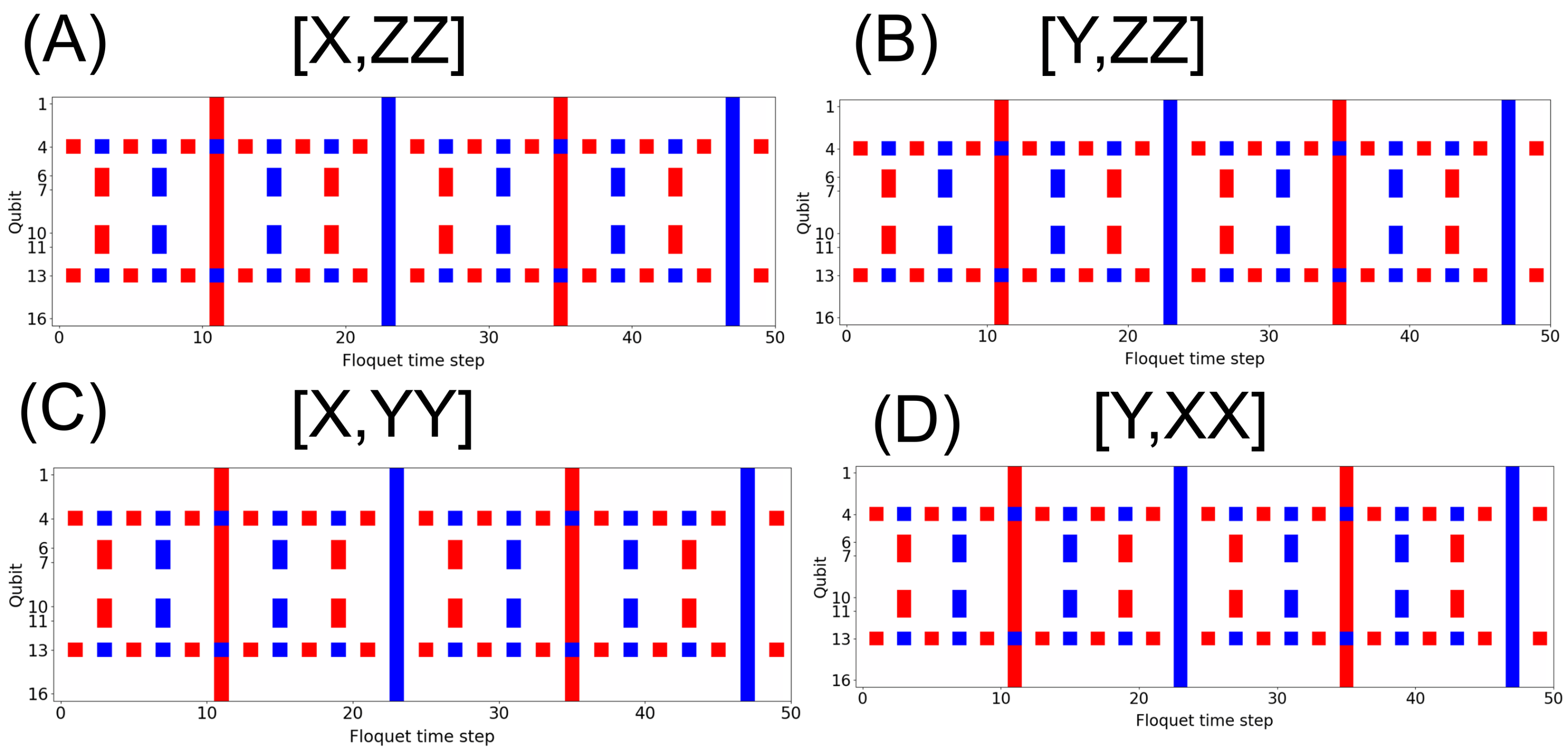
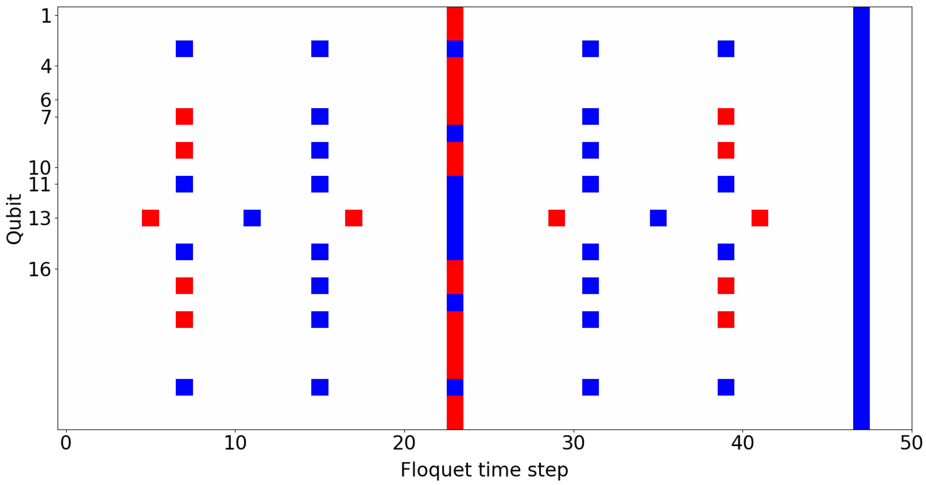
Figure 2.
A 2D Polarization measurement. The polarization measurement, = , of each qubit for 16 time steps, , in the DTC state, with and for rotations in the X axis and ZZ interactions. Red, |1〉; blue, |0〉.
Figure 2.
A 2D Polarization measurement. The polarization measurement, = , of each qubit for 16 time steps, , in the DTC state, with and for rotations in the X axis and ZZ interactions. Red, |1〉; blue, |0〉.

Figure 3.
Thermalization. The polarization measurement, = , of each qubit for each time step, t, in the system, with for the ZZ interaction and = 0 with (A) g(1 − 0.99), (B) g(1 − 0.9), (C) g(1 − 0.75), (D) g(1 − 0.5). Red, |1〉; blue, |0〉.
Figure 3.
Thermalization. The polarization measurement, = , of each qubit for each time step, t, in the system, with for the ZZ interaction and = 0 with (A) g(1 − 0.99), (B) g(1 − 0.9), (C) g(1 − 0.75), (D) g(1 − 0.5). Red, |1〉; blue, |0〉.

Figure 4.
Onsite disorder. The polarization measurement, = , of each qubit for each time step, t, in the system, with for the ZZ interactions and g = 5 with parameters (A) = 0.01, (B) = 0.1, (C) = 0.25, (D) = 0.5. Red, |1〉; blue, |0〉.
Figure 4.
Onsite disorder. The polarization measurement, = , of each qubit for each time step, t, in the system, with for the ZZ interactions and g = 5 with parameters (A) = 0.01, (B) = 0.1, (C) = 0.25, (D) = 0.5. Red, |1〉; blue, |0〉.
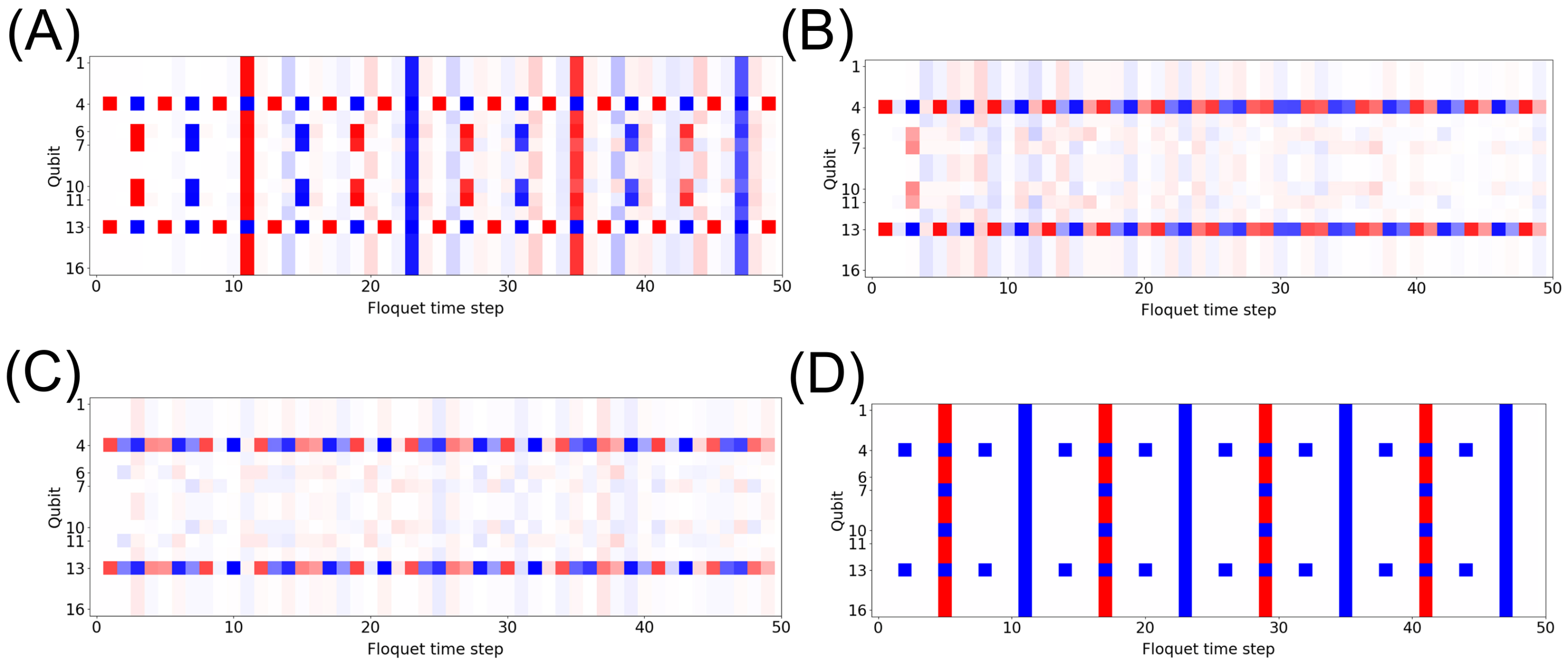
Figure 5.
A 2D DTC circuit. An example of a 2D DTC crystal algorithm with 4 qubits implemented, which results in a 2 × 2 square with interacting qubits. This algorithm is repeated for t Bloch–Floquet time steps and then measured at the end. All qubits are initialized to |0〉.
Figure 5.
A 2D DTC circuit. An example of a 2D DTC crystal algorithm with 4 qubits implemented, which results in a 2 × 2 square with interacting qubits. This algorithm is repeated for t Bloch–Floquet time steps and then measured at the end. All qubits are initialized to |0〉.

Disclaimer/Publisher’s Note: The statements, opinions and data contained in all publications are solely those of the individual author(s) and contributor(s) and not of MDPI and/or the editor(s). MDPI and/or the editor(s) disclaim responsibility for any injury to people or property resulting from any ideas, methods, instructions or products referred to in the content. |
© 2023 by the author. Licensee MDPI, Basel, Switzerland. This article is an open access article distributed under the terms and conditions of the Creative Commons Attribution (CC BY) license (https://creativecommons.org/licenses/by/4.0/).
Share and Cite
MDPI and ACS Style
Sims, C. Formation of Tesseract Time Crystals on a Quantum Computer. Crystals 2023, 13, 1265. https://doi.org/10.3390/cryst13081265
AMA Style
Sims C. Formation of Tesseract Time Crystals on a Quantum Computer. Crystals. 2023; 13(8):1265. https://doi.org/10.3390/cryst13081265
Chicago/Turabian StyleSims, Christopher. 2023. "Formation of Tesseract Time Crystals on a Quantum Computer" Crystals 13, no. 8: 1265. https://doi.org/10.3390/cryst13081265
Note that from the first issue of 2016, this journal uses article numbers instead of page numbers. See further details here.