
Twin Peaks: Interrogating Otolith Pairs to See Whether They Keep Their Stories Straight


Abstract
1. Introduction
2. Materials and Methods
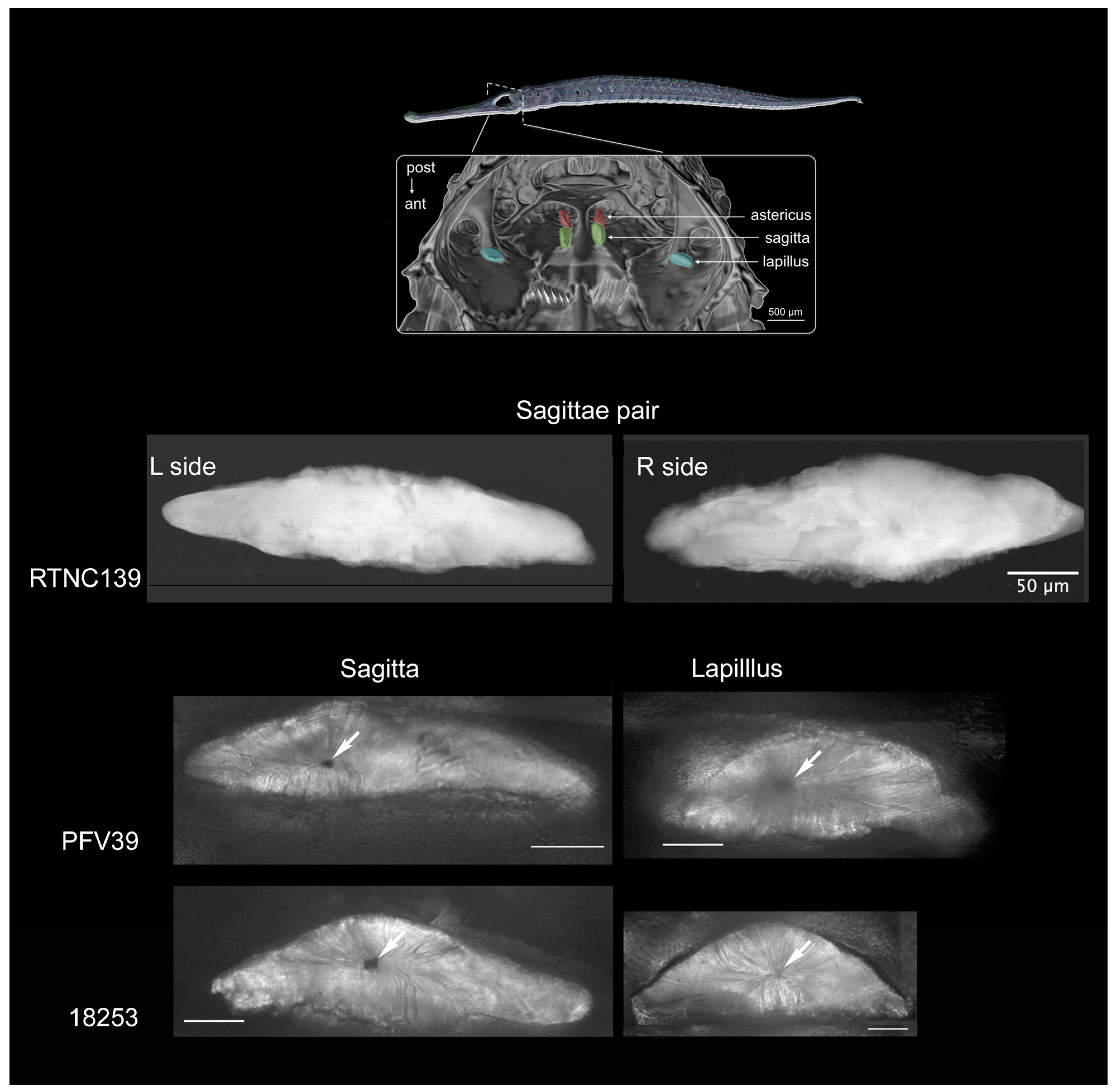
2.1. Sample Preparation
2.2. Synchrotron-Induced X-ray Fluorescence Scanning
2.3. Element Distribution Analysis
2.4. Sr:Ca Molar Ratio Processing
2.5. Trace Elements
2.6. Sulphur and Increment Addressing
3. Results
3.1. Global and Hyperfine Sr Integration in the Otoliths
3.2. Sulphur-Based Counting of Growth Increments
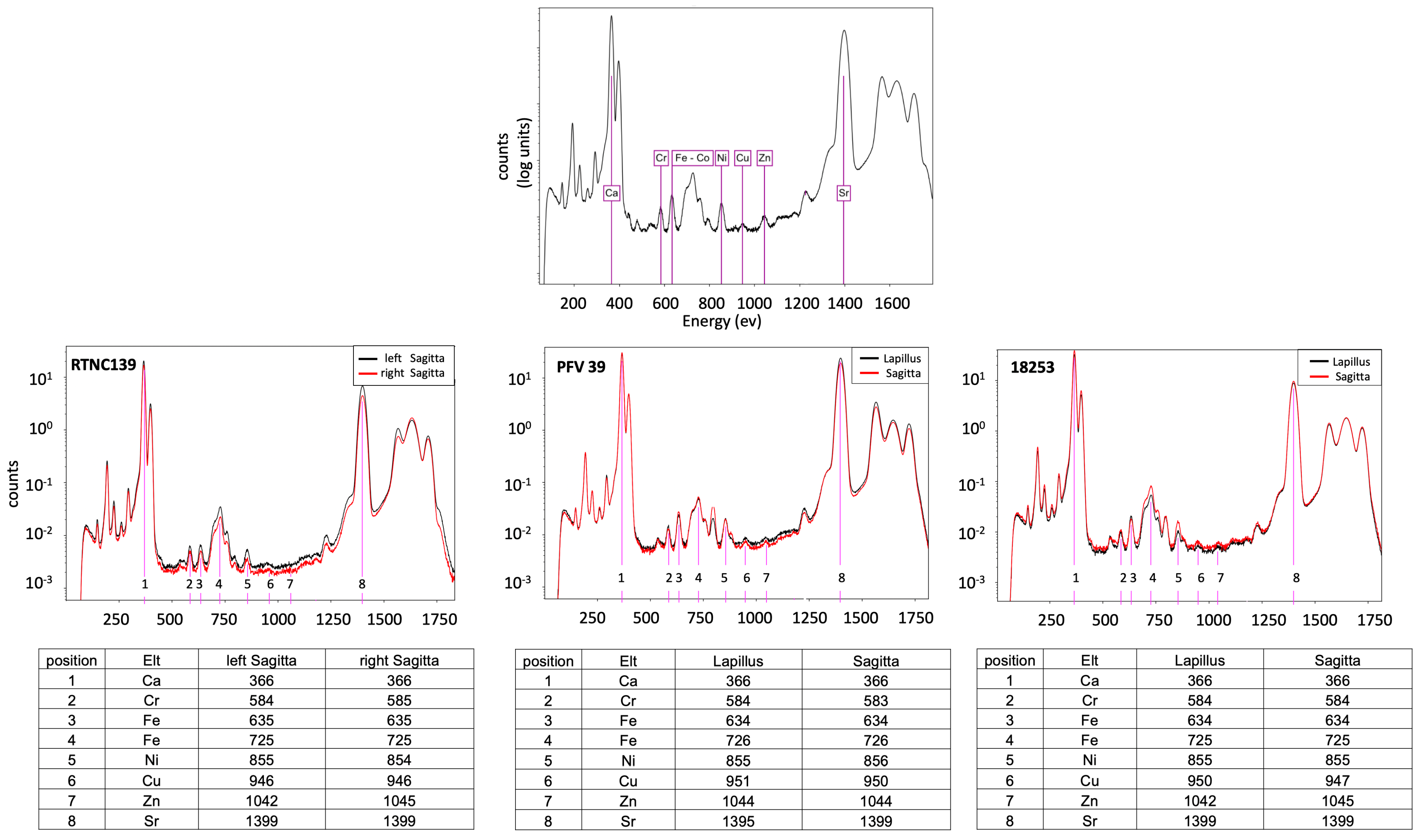
3.3. Trace Element Distribution
4. Discussion
4.1. Sr/Ca Global Maps
4.2. Sulphur Peaks
4.3. Trace Element Incorporation
4.4. Cues from Specific Location and Concentration Patterns of Trace Metal Elements
4.4.1. Zinc Incorporation
4.4.2. Zinc as a Proxy of Biomineralization Processes
4.4.3. Zinc Localisation and Otolith Element Patchiness
4.4.4. Integrated Chemical and Biological Processes
5. Conclusions
Author Contributions
Funding
Data Availability Statement
Acknowledgments
Conflicts of Interest
References
- Schulz-Mirbach, T.; Ladich, F.; Plath, M.; Heß, M. Enigmatic ear stones: What we know about the functional role and evolution of fish otoliths. Biol. Rev. 2019, 94, 457–482. [Google Scholar] [CrossRef] [PubMed]
- Popper, A.N.; Fay, R.R. Sound detection and processing by fish: Critical review and major research questions (part 2 of 2). Brain Behav. Evol. 1993, 41, 26–38. [Google Scholar] [CrossRef]
- Anken, R.H.; Ibsch, M.; Breuer, J.; Rahmann, H. Effect of hypergravity on the Ca/Sr composition of developing otoliths of larval cichlid fish (Oreochromis mossambicus). Comp. Biochem. Physiol. Part A Mol. Integr. 2001, 128, 369–377. [Google Scholar] [CrossRef] [PubMed]
- Inoue, M.; Tanimoto, M.; Oda, Y. The role of ear stone size in hair cell acoustic sensory transduction. Sci. Rep. 2013, 3, 2114. [Google Scholar] [CrossRef] [PubMed]
- Dunkelberger, D.G.; Dean, J.M.; Watabe, N. The ultrastructure of the otolithic membrane and otolith in the juvenile mummichog, Fundulus heteroclitus. J. Morphol. 1980, 163, 367–377. [Google Scholar] [CrossRef] [PubMed]
- Lychakov, D.V.; Rebane, Y.T.; Lombarte, A.; Fuiman, L.A.; Takabayashi, A. Fish otolith asymmetry: Morphometry and modeling. Hear. Res. 2006, 219, 1–11. [Google Scholar] [CrossRef] [PubMed]
- Campana, S.E. Chemistry and composition of fish otoliths: Pathways, mechanisms, and applications. Mar. Ecol. Prog. Ser. 1999, 188, 263–297. [Google Scholar] [CrossRef]
- Campana, S.E.; Thorrold, S.R. Otoliths, increments, and elements: Keys to a comprehensive understanding of fish populations? Can. J. Fish. Aquat. Sci. 2001, 58, 30–38. [Google Scholar] [CrossRef]
- Lecomte-Finiger, R. L‘otolithe: La ≪boîte noire≫ des Téléostéens. Annee. Biol. 1999, 38, 107–122. [Google Scholar] [CrossRef]
- Bergenius, M.A.; McCormick, M.I.; Meekan, M.G.; Robertson, D.R. Environmental influences on larval duration, growth and magnitude of settlement of a coral reef fish. Mar. Biol. 2005, 147, 291–300. [Google Scholar] [CrossRef]
- Grammer, G.L.; Morrongiello, J.R.; Izzo, C.; Hawthorne, P.J.; Middleton, J.F.; Gillanders, B.M. Coupling biogeochemical tracers with fish growth reveals physiological and environmental controls on otolith chemistry. Ecol. Monogr. 2017, 87, 487–507. [Google Scholar] [CrossRef]
- Haÿ, V.; Berland, S.; Medjoubi, K.; Somogyi, A.; Mennesson, M.I.; Keith, P.; Lord, C. Unmasking pipefish otolith using synchrotron-based scanning X-ray fluorescence. Sci. Rep. 2023, 13, 4794. [Google Scholar] [CrossRef] [PubMed]
- de Pontual, H.; MacKenzie, K.M.; Tabouret, H.; Daverat, F.; Mahé, K.; Pecheyran, C.; Hüssy, K. Heterogeneity of Otolith Chemical Composition from Two-Dimensional Mapping: Relationship with biomineralization mechanisms and implications for microchemistry analyses. J. Fish. Biol. 2024, 104, 20–33. [Google Scholar] [CrossRef] [PubMed]
- Lord, C.; Haÿ, V.; Medjoubi, K.; Berland, S.; Keith, P. Travelling in Microphis (Teleostei: Syngnathidae) Otoliths with Two-Dimensional X-ray Fluorescence Maps: Twists and Turns on the Road to Strontium Incorporation. Biology 2024, 13, 446. [Google Scholar] [CrossRef] [PubMed]
- Zimmerman, C.E. Relationship of otolith strontium-to-calcium ratios and salinity: Experimental validation for juvenile salmonids. Can. J. Fish. Aquat. Sci. 2005, 62, 88–97. [Google Scholar] [CrossRef]
- Zimmerman, C.E.; Swanson, H.K.; Volk, E.C.; Kent, A.J. Species and Life History Affect the Utility of Otolith Chemical Composition for Determining Natal Stream of Origin for Pacific Salmon. Trans. Am. Fish. Soc. 2013, 142, 1370–1380. [Google Scholar] [CrossRef]
- Parkinson, K.L.; Booth, D.J.; Lee, J.E. Validation of otolith daily increment formation for two temperate syngnathid fishes: The pipefishes Stigmatopora argus and Stigmatopora nigra. J. Fish Biol. 2012, 80, 698–704. [Google Scholar] [CrossRef] [PubMed]
- Lowenstam, H.A. Minerals formed by organisms. Science 1981, 211, 1126–1131. [Google Scholar] [CrossRef]
- Hüssy, K.; Limburg, K.E.; de Pontual, H.; Thomas, O.R.B.; Cook, P.K.; Heimbrand, Y.; Blass, M.; Sturrock, A.M. Trace Element Patterns in Otoliths: The Role of Biomineralization. Rev. Fish. Sci. Aquac. 2021, 29, 445–477. [Google Scholar] [CrossRef]
- de Goeyse, S.; Webb, A.E.; Reichart, G.J.; de Nooijer, L.J. Carbonic anhydrase is involved in calcification by the benthic foraminifer Amphistegina lessonii. Biogeosciences 2021, 18, 393–401. [Google Scholar] [CrossRef]
- Smith, N.G.; Jones, C.M. Substituting otoliths for chemical analyses: Does sagitta = lapillus? Mar. Ecol. Prog. Ser. 2006, 313, 241–247. [Google Scholar] [CrossRef]
- Hedges, K.J.; Ludsin, S.A.; Frayer, B.J. Effects of ethanol preservation on otolith microchemistry. J. Fish Biol. 2004, 64, 923–937. [Google Scholar] [CrossRef]
- Somogyi, A.; Medjoubi, K.; Baranton, G.; Le Roux, V.; Ribbens, M.; Polack, F.; Philippot, P.; Samama, J.P. Optical design and multi-length-scale scanning spectro-microscopy possibilities at the Nanoscopium beamline of Synchrotron Soleil. J. Synchrotron Rad. 2015, 22, 1118–1129. [Google Scholar] [CrossRef] [PubMed]
- Medjoubi, K.; Leclercq, N.; Langlois, F.; Buteau, A.; Lé, S.; Poirier, S.; Mercère, P.; Sforna, M.C.; Kewish, C.M.; Somogyi, A. Development of fast, simultaneous and multi-technique scanning hard X-ray microscopy at Synchrotron Soleil. J. Synchrotron Rad. 2013, 20, 293–299. [Google Scholar] [CrossRef] [PubMed]
- Bergamaschi, A.; Medjoubi, K.; Messaoudi, C.; Marco, S.; Somogyi, A. MMX-I: Data-processing software for multimodal X-ray imaging and tomography. J. Synchrotron Rad. 2016, 23, 783–794. [Google Scholar] [CrossRef] [PubMed]
- Fiji. Available online: http://fiji.sc/cgi-bin/gitweb.cgi (accessed on 5 June 2024).
- Schindelin, J.; Arganda-Carreras, I.; Frise, E.; Kaynig, V.; Longair, M.; Pietzsch, T.; Preibisch, S.; Rueden, C.; Saaldfeld, S.; Schmid, B.; et al. Fiji: An open-source platform for biological-image analysis. Nat. Methods 2012, 9, 676–682. [Google Scholar] [CrossRef] [PubMed]
- PyMca, version 5.9.2; European Synchrotron Radiation Facility: Grenoble, France, 2004. Available online: http://pymca.sourceforge.net/ (accessed on 6 June 2024).
- Solé, V.A.; Papillon, E. PyMca–X-Ray Spectrum Analysis in Python; European Synchrotron Radiation Facility (ESRF): Grenoble, France, 2004; p. 38043. [Google Scholar]
- Solé, V.A.; Papillon, E.; Cotte, M.; Walter, P.; Susini, J.A.A. Multiplatform Code for the Analysis of Energy-Dispersive X-Ray Fluorescence Spectra. Spectroc. Acta Part B At. Spectrosc. 2007, 62, 63–68. [Google Scholar] [CrossRef]
- R Development Core Team. R, version 4.2.3; R Foundation for Statistical Computing: Vienna, Austria, 2020. Available online: https://www.R-project.org/ (accessed on 15 March 2023).
- Keith, P. Biology and Ecology of Amphidromous Gobiidae of the Indo-Pacific and the Caribbean Regions. J. Fish. Biol. 2003, 63, 831–847. [Google Scholar] [CrossRef]
- Potter, I.C.; Tweedley, J.R.; Elliott, M.; Whitfield, A.K. The ways in which fish use estuaries: A refinement and expansion of the guild approach. Fish Fish. 2015, 16, 230–239. [Google Scholar] [CrossRef]
- Elsdon, T.S.; Gillanders, B.M. Consistency of patterns between laboratory experiments and field collected fish in otolith chemistry: An example and applications for salinity reconstructions. Mar. Freshwater Res. 2005, 56, 609–617. [Google Scholar] [CrossRef]
- Thomas, O.R.B.; Ganio, K.; Roberts, B.R.; Swearer, S.E. Trace element–protein interactions in endolymph from the inner ear of fish: Implications for environmental reconstructions using fish otolith chemistry. Metallomics 2017, 9, 239–249. [Google Scholar] [CrossRef] [PubMed]
- Jessop, B.; Cairns, D.; Thibault, I.; Tzeng, W. Life history of American eel Anguilla rostrata: New insights from otolith microchemistry. Aquat. Biol. 2008, 1, 205–216. [Google Scholar] [CrossRef]
- Brown, R.J.; Severin, K.P. Otolith chemistry analyses indicate that water Sr:Ca is the primary factor influencing otolith Sr:Ca for freshwater and diadromous fish but not for marine fish. Can. J. Fish. Aquat. Sci. 2009, 66, 1790–1808. [Google Scholar] [CrossRef]
- McFadden, A.; Wade, B.; Izzo, C.; Gillanders, B.M.; Lenehan, C.E.; Pring, A. Quantitative electron microprobe mapping of otoliths suggests elemental incorporation is affected by organic matrices: Implications for the interpretation of otolith chemistry. Mar. Freshw. Res. 2015, 67, 889–898. [Google Scholar] [CrossRef]
- Borelli, G.; Guibbolini, M.E.; Mayer-Gostan, N.; Priouzeau, F.; De Pontual, H.; Allemand, D.; Puverel, S.; Tambutte, E.; Payan, P. Daily variations of endolymph composition: Relationship with the otolith calcification process in trout. J. Exp. Biol. 2003, 206, 2685–2692. [Google Scholar] [CrossRef] [PubMed]
- Arias, J.L.; Neira-Carrillo, A.; Arias, J.I.; Escobar, C.; Bodero, M.; David, M.; Fernandez, M.S. Sulfated polymers in biological mineralization: A plausible source for bioinspired engineering. J. Mater. Chem. 2004, 14, 2154–2160. [Google Scholar] [CrossRef]
- Iida, M.; Watanabe, S.; Tsukamoto, K. Oceanic larval duration and recruitment mechanism of the amphidromous fish Sicyopterus japonicus (Gobioidei: Sicydiinae). Reg. Stud. Mar. Sci. 2015, 1, 25–33. [Google Scholar] [CrossRef]
- Bounket, B.; Gibert, P.; Gennotte, V.; Argillier, C.; Carrel, G.; Maire, A.; Logez, M.; Morat, F. Otolith shape analysis and daily increment validation during ontogeny of larval and juvenile European chub Squalius cephalus. J. Fish Biol. 2019, 95, 444–452. [Google Scholar] [CrossRef] [PubMed]
- Fey, D.P.; Lejk, A.M.; Greszkiewicz, M. Daily deposition of growth increments in sagittae and lapilli of laboratory-reared larval northern pike (Esox lucius). Fish. Bull. 2018, 116, 302–309. [Google Scholar] [CrossRef]
- Morioka, S.; Machinandiarena, L. Comparison of daily increment formation pattern between sagittae and lapilli of ling (Genypterus blacodes) larvae and juveniles collected off Argentina. N. Z. J. Mar. Freshw. Res. 2001, 35, 111–119. [Google Scholar] [CrossRef]
- Campana, S.E. Photographic Atlas of Fish Otoliths of the Northwest Atlantic Ocean, In Canadian Special Publication of Fisheries and Aquatic Sciences; NRC Research Press: Ottawa, Canada, 2004; Volume 133, pp. 1–11. [Google Scholar]
- Morales-Nin, B. Review of the growth regulation processes of otolith daily increment formation. Fish. Res. 2000, 46, 53–67. [Google Scholar] [CrossRef]
- Hüssy, K. Otolith shape in juvenile cod (Gadus morhua): Ontogenetic and environmental effects. J. Exp. Mar. Bio. Ecol. 2008, 364, 35–41. [Google Scholar] [CrossRef]
- Vignon, M.; Morat, F. Environmental and genetic determinant of otolith shape revealed by a non-indigenous tropical fish. Mar. Ecol. Prog. Ser. 2010, 411, 231–241. [Google Scholar] [CrossRef]
- Vignon, M. Ontogenetic trajectories of otolith shape during shift in habitat use: Interaction between otolith growth and environment. J. Exp. Mar. Bio. Ecol. 2012, 420, 26–32. [Google Scholar] [CrossRef]
- Baumann, H.; Gagliano, M. Changing otolith/fish size ratios during settlement in two tropical damselfishes. Helgol. Mar. Res. 2011, 65, 425–429. [Google Scholar] [CrossRef]
- Protasowicki, M.; Kosior, M. Long-term observations of selected heavy metals contained in otoliths of cod from the Southern Baltic. Kieler Meeresforsch. Sonderh. 1988, 6, 424–431. [Google Scholar]
- Arslan, Z.; Secor, D.H. Analysis of trace transition elements and heavy metals in fish otoliths as tracers of habitat use by American eels in the Hudson River estuary. Estuaries 2005, 28, 382–393. [Google Scholar] [CrossRef]
- Hansson, S.V.; Desforges, J.P.; van Beest, F.M.; Bach, L.; Halden, N.M.; Sonne, C.; Mosbech, A.; Søndergaard, J. Bioaccumulation of mining derived metals in blood, liver, muscle and otoliths of two Arctic predatory fish species (Gadus ogac and Myoxocephalus scorpius). Environ. Res. 2020, 183, 109194. [Google Scholar] [CrossRef] [PubMed]
- Daros, F.A.; Condini, M.V.; Altafin, J.P.; de Oliveira Ferreira, F.; Hostim-Silva, M. Fish otolith microchemistry as a biomarker of the world’s largest mining disaster. Sci. Total Environ. 2022, 807, 151780. [Google Scholar] [CrossRef] [PubMed]
- Sturrock, A.M.; Hunter, E.; Milton, J.A.; EIMF; Johnson, R.C.; Waring, C.P.; Trueman, C.N. Quantifying physiological influences on otolith microchemistry. Methods Ecol. Evol. 2015, 6, 806–816. [Google Scholar] [CrossRef]
- Miller, P.A.; Munkittrick, K.R.; Dixon, D.G. Relationship between concentrations of copper and zinc in water, sediment, benthic invertebrates, and tissues of white sucker (Catostomus commersoni) at metal-contaminated sites. Can. J. Fish. Aquat. Sci. 1992, 49, 978–984. [Google Scholar] [CrossRef]
- Pender, P.J.; Griffin, R.K. Habitat history of barramundi Lates calcarifer in a north Australian river system based on barium and strontium levels in scales. T. Am. Fish. Soc. 1996, 125, 679–689. [Google Scholar] [CrossRef]
- Daverat, F.; Lanceleur, L.; Pécheyran, C.; Eon, M.; Dublon, J.; Pierre, M.; Schäfer, J.; Baudrimont, M.; Renault, S. Accumulation of Mn, Co, Zn, Rb, Cd, Sn, Ba, Sr, and Pb in the otoliths and tissues of eel (Anguilla anguilla) following long-term exposure in an estuarine environment. Sci. Total Environ. 2012, 437, 323–330. [Google Scholar] [CrossRef] [PubMed]
- Andronis, C.; Evans, N.J.; McDonald, B.J.; Nice, H.E.; Gagnon, M.M. Otolith microchemistry: Insights into bioavailable pollutants in a man-made, urban inlet. Mar. Pollut. Bull. 2017, 118, 382–387. [Google Scholar] [CrossRef] [PubMed]
- Fowler, A.J.; Campana, S.E.; Thorrold, S.R.; Jones, C.M. Experimental assessment of the effect of temperature and salinity on elemental composition of otoliths using solution-based ICPMS. Can. J. Fish. Aquat. Sci. 1995, 52, 1421–1430. [Google Scholar] [CrossRef]
- Forrester, G.E. A field experiment testing for correspondence between trace elements in otoliths and the environment and for evidence of adaptation to prior habitats. Estuaries 2005, 28, 974–981. [Google Scholar] [CrossRef]
- Hicks, A.S.; Closs, G.P.; Swearer, S.E. Otolith microchemistry of two amphidromous galaxiids across an experimental salinity gradient: A multi-element approach for tracking diadromous migrations. J. Exp. Mar. Bio. Ecol. 2010, 394, 86–97. [Google Scholar] [CrossRef]
- Gauldie, R.W.; Nathan, A. Iron content of the otoliths of tarakihi (Teleostei: Cheilodactylidae). N. Z. J. Mar. Freshw. Res. 1977, 11, 179–191. [Google Scholar] [CrossRef]
- Begg, G.A.; Cappo, M.; Boyle, S. Waters of eastern Australia by analysis of minor and trace. Fish. Bull. 1998, 96, 653–666. [Google Scholar]
- Keith, P.; Lord, C.; Maeda, K. Indo-Pacific Sicydiine Gobies: Biodiversity, Life Traits and Conservation; Société Française d’Ichtyologie: Paris, France, 2015. [Google Scholar]
- Perfetto, R.; Del Prete, S.; Vullo, D.; Sansone, G.; Barone, C.; Rossi, M.; Capasso, C. Biochemical characterization of the native α-carbonic anhydrase purified from the mantle of the Mediterranean mussel, Mytilus galloprovincialis. J. Enzyme Inhib. Med. Chem. 2017, 32, 632–639. [Google Scholar] [CrossRef] [PubMed]
- de Nooijer, L.J.; Toyofuku, T.; Kitazato, H. Foraminifera promote calcification by elevating their intracellular pH. Proc. Natl. Acad. Sci. USA 2009, 106, 15374–15378. [Google Scholar] [CrossRef] [PubMed]
- Borelli, G.; Mayer-Gostan, N.; De Pontual, H.; Boeuf, G.; Payan, P. Biochemical relationships between endolymph and otolith matrix in the trout (Oncorhynchus mykiss) and turbot (Psetta maxima). Calcif. Tissue Int. 2001, 69, 356–364. [Google Scholar] [CrossRef] [PubMed]
- Payan, P.; De Pontual, H.; Bœuf, G.; Mayer-Gostan, N. Endolymph chemistry and otolith growth in fish. C. R. Palevol 2004, 3, 535–547. [Google Scholar] [CrossRef]


| Species | ID | Collection N° | SL | Country | River | Otolith Pair |
|---|---|---|---|---|---|---|
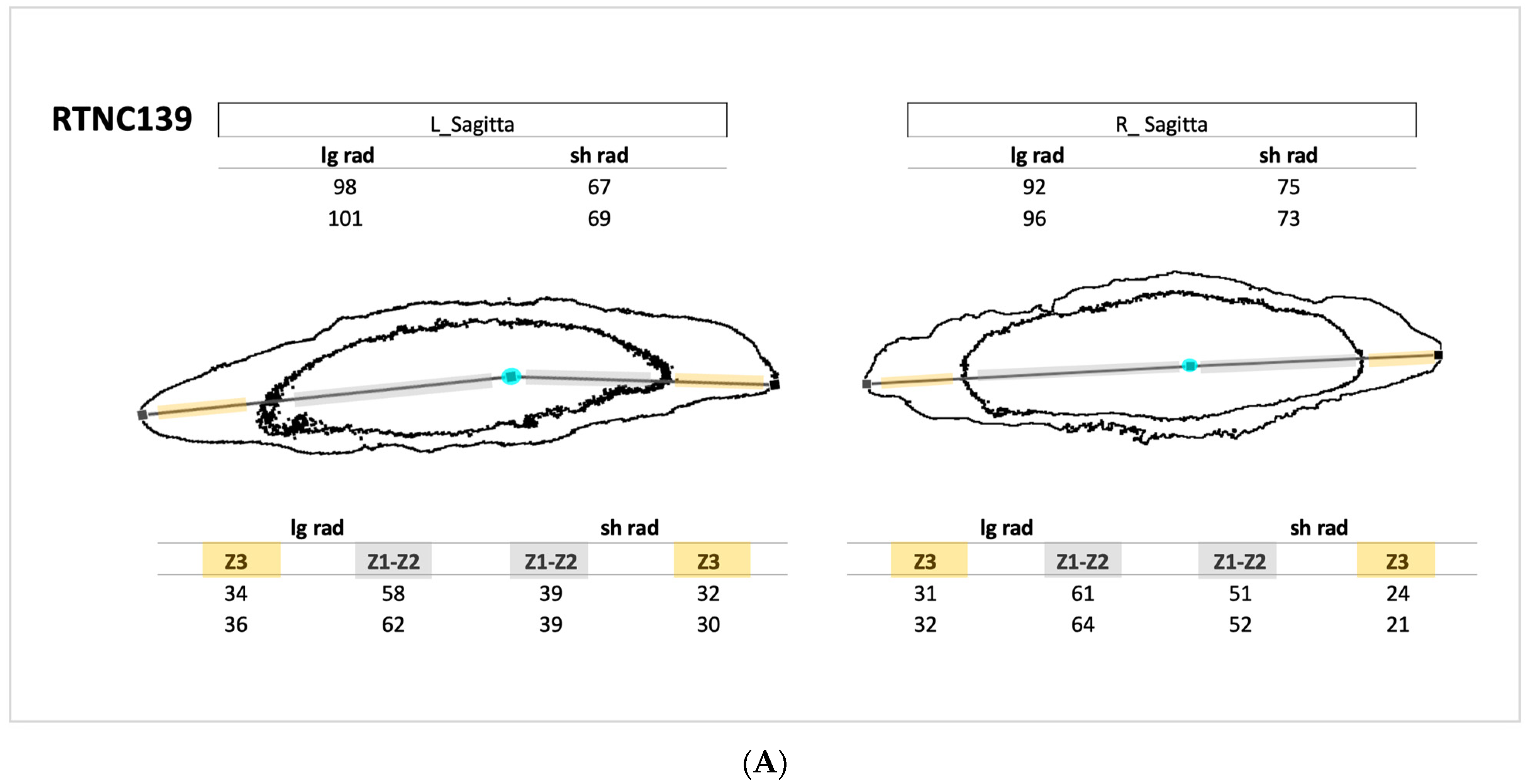
| Microphis brachyurus | RTNC139 | MNHN-IC-2021-0322 | 105.57 | New Caledonia | Garana | Left Sagitta Right Sagitta |
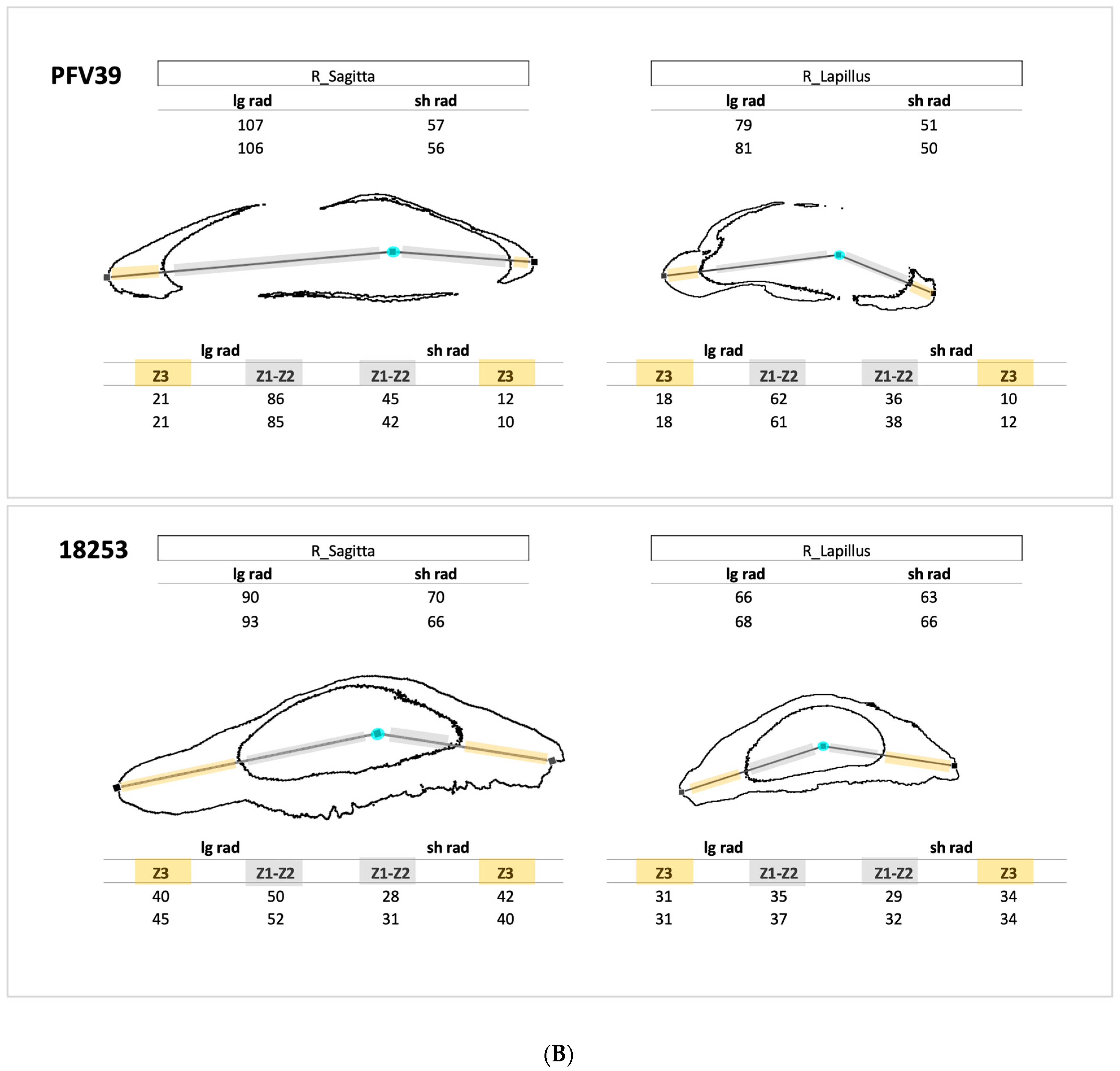
| Microphis brachyurus | PFV39 | MNHN-IC-2023-0052 | 109.36 | French Polynesia | Papenoo | Right Sagitta Right Lapillus |
| Microphis nicoleae | 18253 | MNHN-IC-2023-0047 | 97.65 | Solomon Islands | Rakata | Right Sagitta Right Lapillus |
Disclaimer/Publisher’s Note: The statements, opinions and data contained in all publications are solely those of the individual author(s) and contributor(s) and not of MDPI and/or the editor(s). MDPI and/or the editor(s) disclaim responsibility for any injury to people or property resulting from any ideas, methods, instructions or products referred to in the content. |
© 2024 by the authors. Licensee MDPI, Basel, Switzerland. This article is an open access article distributed under the terms and conditions of the Creative Commons Attribution (CC BY) license (https://creativecommons.org/licenses/by/4.0/).
Share and Cite
Lord, C.; Berland, S.; Haÿ, V.; Medjoubi, K.; Keith, P. Twin Peaks: Interrogating Otolith Pairs to See Whether They Keep Their Stories Straight. Crystals 2024, 14, 705. https://doi.org/10.3390/cryst14080705
Lord C, Berland S, Haÿ V, Medjoubi K, Keith P. Twin Peaks: Interrogating Otolith Pairs to See Whether They Keep Their Stories Straight. Crystals. 2024; 14(8):705. https://doi.org/10.3390/cryst14080705
Chicago/Turabian StyleLord, Clara, Sophie Berland, Vincent Haÿ, Kadda Medjoubi, and Philippe Keith. 2024. "Twin Peaks: Interrogating Otolith Pairs to See Whether They Keep Their Stories Straight" Crystals 14, no. 8: 705. https://doi.org/10.3390/cryst14080705
APA StyleLord, C., Berland, S., Haÿ, V., Medjoubi, K., & Keith, P. (2024). Twin Peaks: Interrogating Otolith Pairs to See Whether They Keep Their Stories Straight. Crystals, 14(8), 705. https://doi.org/10.3390/cryst14080705