Exploring the Premelting Transition through Molecular Simulations Powered by Neural Network Potentials

Abstract

The premelting layer on crystal surfaces significantly affects the stability, surface reactivity, and phase transition behaviors of crystals. Traditional methods for studying this layer—experimental techniques, classical simulations, and even first-principle simulations—have significant limitations in accuracy and scalability. To overcome these challenges, we employ molecular dynamic simulations based on neural network potentials to investigate the structural and dynamic behavior of the premelting layer on ice. This approach matches the accuracy of first-principle calculations while greatly improving computational efficiency, allowing us to simulate the ice–vapor interface on a much larger scale. In this study, we conducted a one-nanosecond simulation of the ice–vapor interface involving 1024 water molecules. This significantly exceeds the time and size scales of previous first-principle studies. Our simulation results indicate complete surface melting. Furthermore, our simulation results reveal dynamic heterogeneity within the premelting layer, with molecules segregated into clusters of low and high mobility.

1. Introduction

The surface of ice in contact with air is covered by a thin film of liquid water, known as the premelting layer. Initially proposed by Faraday in 1842 as an explanation for the reduced friction of ice surfaces [1], the existence of the premelting layer was not empirically confirmed until 1987 [2]. Subsequent research has demonstrated that premelting layers are not unique to ice but also occur on various other crystalline surfaces [3].

The premelting layer plays a crucial role in mediating physical and chemical processes within the atmosphere. Notably, it facilitates the transfer of electrical charges between colliding ice particles in clouds, a mechanism crucial in lightning formation [4]. Additionally, due to its enhanced solubility for ions, the premelting layer serves as a key locus for a variety of atmospheric chemical reactions. For instance, within this layer, hypochlorous acid undergoes conversion to chlorine gas, which subsequently contributes to ozone depletion upon its release into the atmosphere [5]. Similarly, the transformation of atmospheric sulfur dioxide into sulfuric acid within the premelting layer plays key roles in the acidification of snow [6,7].

Recent progress in the field, underpinned by computer simulations and experimental findings, revealed the heterogeneous nature of the premelting layer, indicating it may consist of multiple thermodynamic phases [8,9,10,11,12]. Computer simulation-based studies demonstrate that the layer is not a simple uniform film of liquid water but contains regions that exhibit both liquid-like and solid-like properties, with the ability to transition dynamically between these states [8,9]. Recent experiments show that many droplets emerge on the surface of the premelting layer during the growth of ice crystals [10,11,12]. This has led to the hypothesis that these droplets may represent a distinct thermodynamic phase [10,11,12,13], suggesting a complex structural composition of the premelting layer.

Despite the progress made in understanding the premelting layer, significant uncertainties remain regarding the microscopic mechanisms that dictate its structural and dynamic characteristics. The variation in thickness measurements obtained through different experimental techniques underscores the challenges in accurately characterizing this complex interfacial layer [2,14,15]. Theoretical studies of the premelting layer have largely been based on the Lifshitz theory [16,17,18,19,20]. The most recent application of the Lifshitz theory takes into account dispersion interactions and also incorporates short-ranged correlations such as hydrogen bonding between water molecules [20]. Additionally, the Lifshitz theory has been used to explain the appearance of droplets on the premelting layer during ice crystal growth [21].

In this study, we utilize molecular dynamic simulations enhanced by neural network potentials to probe the premelting layer, aiming to surpass the limitations inherent in experimental methodologies and classical simulation algorithms. Simulations are able to provide insights into the microscopic mechanisms governing the premelting layer, which are often obscured in experimental studies. Traditionally, the field has relied on classical simulation algorithms [8,9,19,22], which are constrained by the use of artificially constructed force fields and the challenges in capturing complex effects, such as the breaking of chemical bonds and electron polarization.

Transitioning to first-principle molecular dynamic simulations addresses these constraints, delivering results that markedly differ from classical approaches [23,24]. However, the computational burden of first-principle simulations limits their application to small-sized systems, thus constraining our ability to draw comprehensive conclusions about the premelting layer’s heterogeneity or thickness near the melting point.

To overcome these limitations, we utilize machine learning-based first-principle simulations, significantly enhancing computational efficiency. Neural network-based potentials, trained on data derived from density functional theory (DFT), is able to not only achieve a level of accuracy on par with the DFT calculations itself [25,26,27,28,29,30,31], but also operate at a significantly higher computational speed [32]. This approach enables us to extend the time and spatial scales of our simulations beyond the reach of conventional DFT-based methods, allowing for a more detailed and accurate exploration of the premelting layer while maintaining first-principles accuracy.

Utilizing the neural network potentials, this work conducts large-scale molecular dynamic simulations to explore the premelting layer at the redvapor–ice interface across varying temperatures. The results indicate that complete surface melting happens as the temperature approaches the bulk ice melting temperature. Furthermore, we observed dynamic heterogeneity within the premelting layer, with molecules segregated into clusters of high and low mobility. This is reminiscent of the behavior seen in supercooled liquids [33].

2. Methods

2.1. Neural Network Potential

In this work, we employed the neural network potential for water molecules developed by Wohlfahrt et al. [34] to simulate the ice–redvapor interface. This potential employs the Behler–Parrinello-style neural network (BPNN), which uses distinct neural networks for each type of atoms within the system. Separate neural networks were designed for the oxygen and hydrogen atoms in water molecules.

Each atomic neural network’s input comprises a set of symmetry functions that characterize the local atomic environment. These functions are designed to remain invariant to translations, rotations, and permutations of identical atoms. For the neural network potential used in this work, Type 2 and Type 4 symmetry functions were used. The Type 2 symmetry function captures the radial distribution of atoms around the central atom, which is defined as

$$G_i^2=\sum _{j\ne i}{e}^{-\eta {(r_{ij}-r_s)}^2}{f}_c\left(r_{ij}\right).$$

(1)

Here, $G_i^2$ represents a Type 2 symmetry function that describes the local environment of atom i. $r_{ij}$ denotes the distance of atom j with respect to atom i. The term $e^{-\eta {(r_{ij}-r_s)}^2}$ is a Gaussian function that assigns a weight to the distance $r_{ij}$ depending on how close $r_{ij}$ is to a reference distance $r_s$ and the width of the Gaussian $\eta$. $f_c\left(r_{ij}\right)$ is a cutoff function, which ensures that only neighbors within a certain distance $r_c$ contribute to $G_i^2$. Its definition is as follows

$$f_c\left(r_{ij}\right)=\left\{\begin{array}{cc}{tanh}^3\left[1-{\displaystyle \frac{r_{ij}}{r_c}}\right]\hfill & \mathrm{with}{r}_{ij}\le r_c\hfill \\ 0\hfill & \mathrm{with}{r}_{ij}>r_c\hfill \end{array}\right.$$

(2)

The Type 4 symmetry function is determined by both the angular and radial distribution of atoms around the central atom, which is defined as

$$G_i^4=2^{1-\zeta }\sum _{j\ne i}\sum _{k\ne i,j}\left[{(1+\lambda cos\left({\alpha }_{ijk}\right))}^{\zeta }\right]e^{-\eta (r_{ij}^2+r_{ik}^2+r_{jk}^2)}{f}_c\left(r_{ij}\right)f_c\left(r_{ik}\right)f_c\left(r_{jk}\right).$$

(3)

Here, ${\alpha }_{ijk}$ is the angle with vertex at atom i, formed by connecting it to neighboring atoms j and k. $\lambda$ and $\zeta$ are parameters that control the contribution of the angle ${\alpha }_{ijk}$ to the symmetry function.

The neural network for the hydrogen atom uses 27 symmetry functions as inputs, whereas the network for the oxygen atom uses 30 symmetry functions. These symmetry functions are obtained by varying the parameters, specifically $r_s$, $\eta$, $\lambda$, $\zeta$ in the definition of the Type 2 and Type 4 symmetry functions. Precise values of the parameters used can be found in ref. [35]. Both networks have a cutoff distance of 6.35 Angstroms, meaning only atoms within this radius from the central atom are considered when calculating the symmetry functions. Previous research indicated that extending this cutoff distance beyond 6.35 Angstroms does not significantly enhance the potential’s accuracy [35].

The neural networks for both hydrogen and oxygen atoms consist of two hidden layers, each containing 25 nodes. The total energy of the water molecule system is computed by summing the energy contributions from each atomic neural network. Each atomic network predicts the energy contribution of its central atom based on the symmetry functions. This energy decomposition allows for an accurate and efficient representation of the potential energy surface of water molecules. The forces experienced by the atoms, essential for conducting molecular dynamics simulations, are derived by computing the gradient of the total energy with respect to the atomic coordinates.

This potential is trained from a comprehensive dataset consisting of 8007 configurations, encompassing a broad spectrum of water states including bulk liquid, bulk ice, water–vapor, and ice–water interfaces. The energy and forces of these configurations are obtained by DFT calculations with the RevPBE functional [36], augmented by Grimme’s D3 correction [37]. These training configurations are processed by the n2p2 software (version 2.2.0) [38,39] to generate the neural network potential. Previous studies [34,35] have shown that this neural network potential can accurately predict properties such as the melting point of ice and the water–vapor coexistence curve, making it an excellent choice for studying the premelting layer. The melting temperature of ice Ih obtained with this potential, denoted as $T_m$, is $274\pm 3$ K [35], which closely matches the experimental value.

2.2. Simulation Settings

The system we simulated consists of a slab of ice in contact with vapor on both sides, as depicted in Figure 1. Periodic boundary conditions are employed to minimize boundary effects. We focused on ice in the Ih phase, which is the most common ice phase found in nature. The initial structure of the iceIh was generated using the GenIce2 software (version 2.2.5.6) [40], arranging the ice into a $4\times 4\times 4$ supercell structure, with each unit cell comprising 16 water molecules. Consequently, the simulated system contains 1024 water molecules, a scale significantly exceeding that of prior first-principle studies on the premelting layer. This enhanced scale allows for a more detailed exploration of the premelting layer’s properties and behaviors under various conditions.

The most common crystal planes of iceIh in contact with vapor are the basal, primary prismatic, and secondary prismatic facets of ice (Figure 2). These different facets are known to affect the thickness of the premelting layer [14]. Therefore, in this work, we separately investigated these specific interfaces of ice in contact with vapor to understand how the unique characteristics of each facet affect the premelting layer.

The molecular dynamic simulations are conducted using the 21Nov2023 version of the LAMMPS software, which has builtin n2p2 support. The simulations are carried out in the NVT ensemble. The time step for the simulation was set to 1fs.

In this work, the ice phase is in contact with vapor on both sides along the z-direction (see Figure 1). Given that the vapor phase is large and contains a minimal number of water molecules, the pressure along the z-direction remains close to zero. However, since the crystal is not in contact with vapor along the x and y directions, the pressure along these two directions will not be zero. To illustrate this point, in Figure 3, we present the pressure tensor as a function of simulation time at 260 K, where the primary prismatic facet is in contact with vapor. The instantaneous pressure tensor exhibits significant fluctuations, which is typical in NVT simulations. However, after time averaging, the time-averaged $P_{zz}$ stays close to zero once the system equilibrates, as expected. In contrast, the time-averaged $P_{xx}$ and $P_{yy}$ approach approximately 300 bar and 450 bar, respectively. The time-averaged off-diagonal elements of the pressure tensor—$P_{xy}$, $P_{yz}$, and $P_{xz}$—remain close to zero. It is important to note that the nonzero pressure along the x and y directions of the crystal may influence premelting behavior.

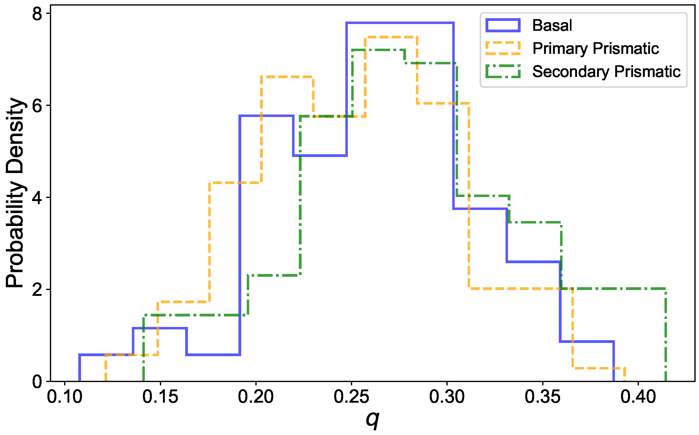
2.3. Local Structural Order Parameter

In this study, we utilized the local structural order parameter proposed by Limmer and Chandler [19] to distinguish whether a water molecule is in a liquid-like or ice-like state. This order parameter was originally developed by Limmer and Chandler to investigate the melting transition at the ice–vapor interface and has proven effective for characterizing the local structural environment of water molecules. It is closely related to the $q_6$ parameter developed by Steinhardt et al. [41] and Lechner et al. [42].

The precise definition of this order parameter is as follows:

$$q^{\left(i\right)}={\displaystyle \frac{1}{4}}{\left(\sum _{m=-6}^6{\left|\sum _{j\in \mathrm{nn}\left(i\right)}{q}_{6m}^{\left(j\right)}\right|}^2\right)}^{1/2},$$

(4)

with

$$q_{6m}^{\left(i\right)}={\displaystyle \frac{1}{4}}\sum _{j\in \mathrm{nn}\left(i\right)}{Y}_{6m}({\varphi }_{ij},{\theta }_{ij}).$$

(5)

Here, $q^{\left(i\right)}$ is the order parameter for the i-th water molecule, represented by its oxygen atom. The summation ${\displaystyle \sum _{j\in \mathrm{nn}\left(i\right)}}$ is performed over the four nearest neighbor oxygens surrounding the central oxygen atom i. The spherical harmonics $Y_{6m}$ are of degree 6, capturing the angular dependence between the central oxygen atom i and its neighboring oxygen atom j. The angles ${\varphi }_{ij}$ and ${\theta }_{ij}$ represent the azimuthal and polar angles, respectively, of the vector connecting these atoms. These functions are crucial for describing the local orientational order.

The construction of q involves averaging the $q_{6m}$ values of neighboring atoms, ensuring that the computed order parameter reflects the local structural information from both the first and second solvation shells.

High values of q typically indicate a local environment resembling the crystalline structure of ice, characterized by a well-defined tetrahedral arrangement. In contrast, lower q values suggest a more disordered, liquid-like state. To determine the criterion value of q that distinguishes liquid-like and ice-like molecules, we performed simulations of bulk ice and bulk liquid separately, using the same neural network potential employed in our study of the ice–vapor interface. The bulk ice simulations were conducted at 175 K, while the bulk liquid simulations were performed at 325 K. The q values obtained from these simulations are summarized in Figure 4. As shown, most liquid-like molecules have q values less than 0.42, whereas most ice-like molecules have q values greater than that threshold. Consequently, we used a criterion value of 0.42 to determine whether a water molecule is ice-like or liquid-like.

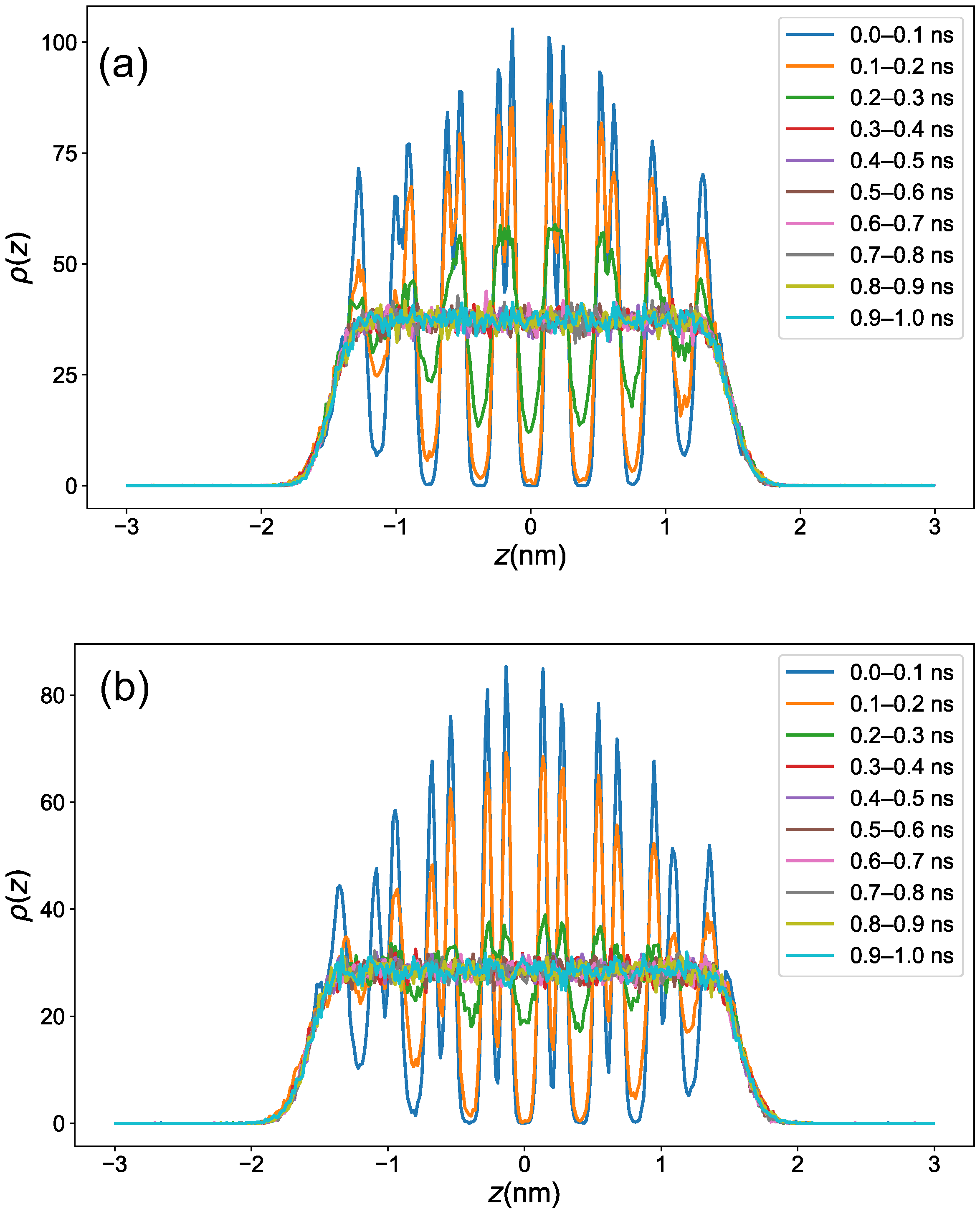
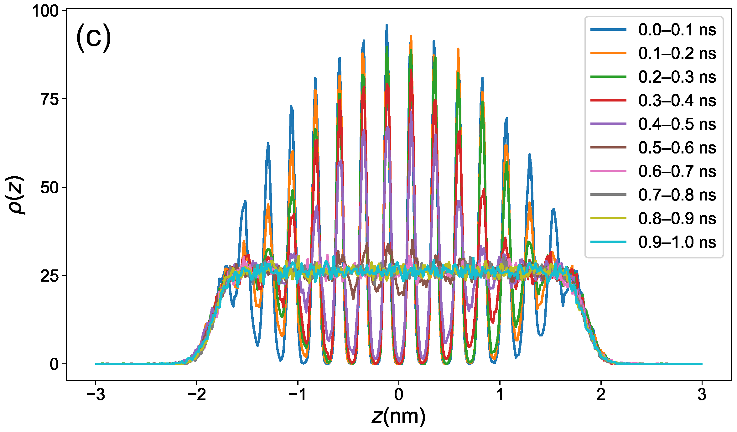
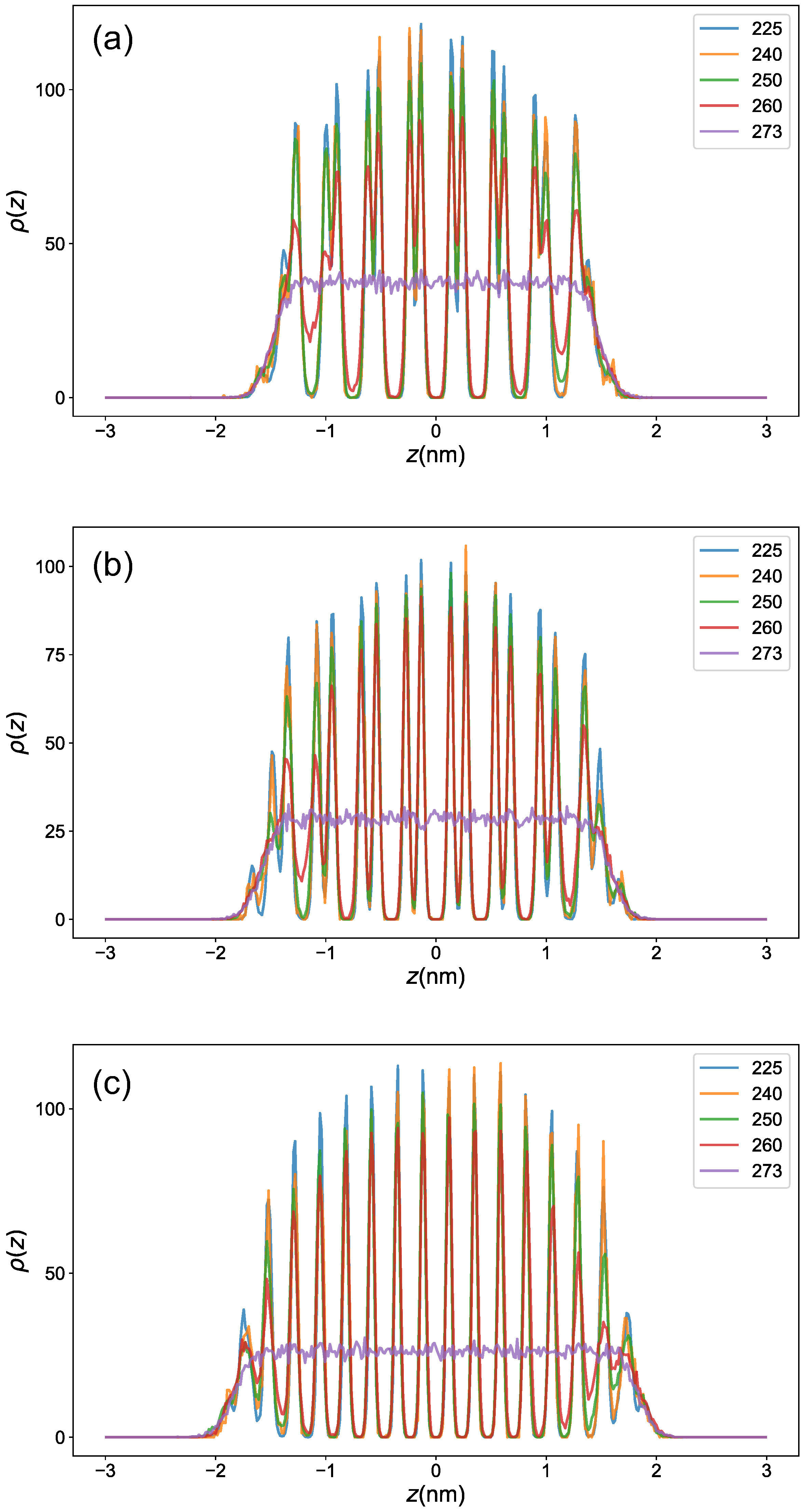
2.4. Density Profile across the Interface

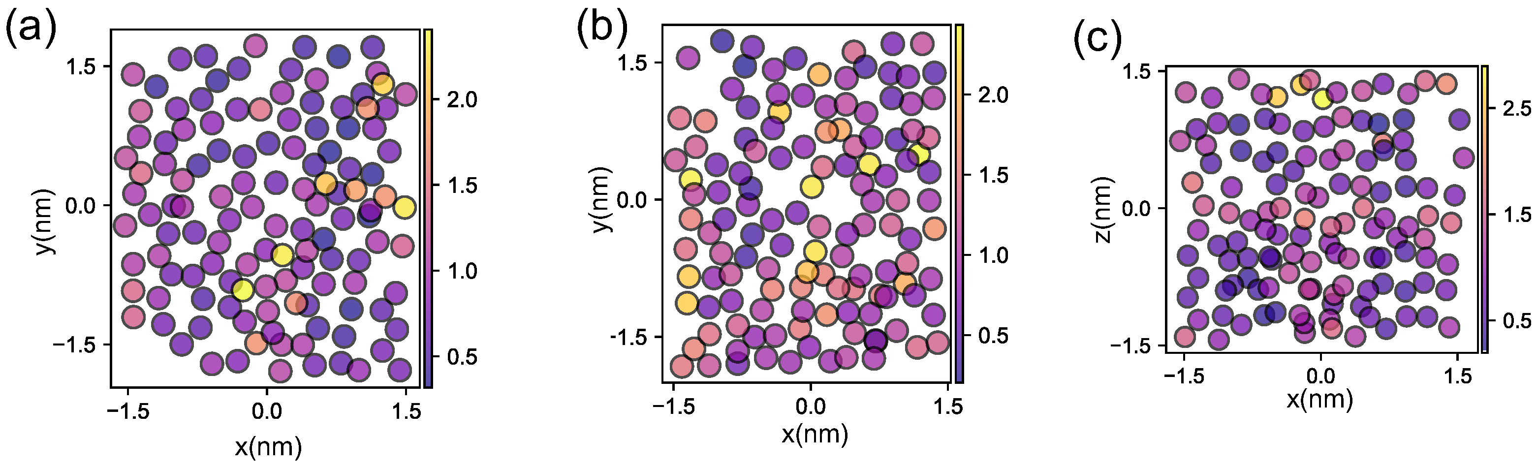
In this work, we analyzed the density profile of oxygen atoms across the vapor–ice interface, which is defined as

$$\rho \left(z\right)={\displaystyle \frac{1}{A}}〈\sum _{i=1}^N\delta (z_i-z)〉,$$

(6)

where A denotes the area of the simulation box in xy plane, $z_i$ is the z-coordinate of the oxygen atom of the i-th molecule, and $〈\cdots 〉$ indicates the ensemble average.

To numerically obtain the density profile $\rho \left(z\right)$, we follow these steps. First, we divide the z-coordinate axis into a series of small bins with width $\Delta z$. For each configuration in the simulation, we count the number of oxygen atoms whose z-coordinates fall within each bin. This counting process is repeated for numerous configurations sampled from the molecular dynamics trajectory. Next, we average the counts over all configurations to smooth out fluctuations. Finally, we normalize the averaged counts by dividing by $A\Delta z$, yielding the density profile $\rho \left(z\right)$.

2.5. Propensity

In this study, we explore the dynamical properties of the premelting layer by examining the molecular propensity within it. Propensity is a well-established metric that gauges the mobility of molecules and is commonly used to identify regions with different mobility for supercooled liquids or glasses, where dynamics can be highly heterogeneous. It is defined as the average squared displacement of each molecule over a time period t [43,44]:

$$\mathrm{propensity}\left(i\right)=\langle \left|\right|r_i\left(t\right)-r_i{\left(0\right)\left|\right|}_2{\rangle }_{\mathrm{iso}}.$$

(7)

Here, i indicates the i-th molecule, identified by its oxygen atom; $r_i\left(t\right)$ marks the position of the molecule’s oxygen atom at time t; and ${\left|\right|\cdots \left|\right|}_2$ denotes the L2 norm. The ${\langle \cdots \rangle }_{\mathrm{iso}}$ notation represents averaging over the isoconfigurational ensemble. This ensemble comprises trajectories that originate from the same structural configuration but diverge due to initial velocities being sampled from a Maxwell distribution. The propensity is obtained by averaging the squared displacement over these paths.

In this particular study, the propensity is obtained by averaging over 10 different trajectories that all start from the same configuration. The time interval t is 100 ps.

3. Results

3.1. Equilibration

To investigate the premelting transition as the temperature approaches the melting temperature, which is $274\pm 3$ K for this neural network potential [35], we performed a series of simulations at temperatures ranging from 225 K to 273 K. We separately simulated cases where the basal, primary prismatic, and secondary prismatic facets of ice are in contact with vapor. For each facet, all simulations at different temperatures started from the perfect crystal form specific to that facet. To ensure the system equilibrates, we conducted 1 ns-long simulations for each trajectory.

To determine whether the system has equilibrated, we plotted the percentage of liquid-like water molecules as a function of simulation time in Figure 5. A water molecule is considered liquid-like if the structural order parameter q is less than 0.42, as discussed in Section 2.3. At the beginning of the simulation, no water molecules are liquid-like since we start from a perfect ice state. As the simulation progresses, some water molecules become liquid-like. The number of liquid-like water molecules stablizes in less than 600 ps for all temperatures investigated, as shown in Figure 5.

We also analyzed the evolution of the oxygen density profile over time. Figure 6 shows the number density profiles across the interface as a function of time at 273 K for the primary prismatic, secondary prismatic, and basal facets. As observed, the number density profiles converges after 600 ps. For all other simulation temperatures, the number density profiles converges even faster than at 273 K.

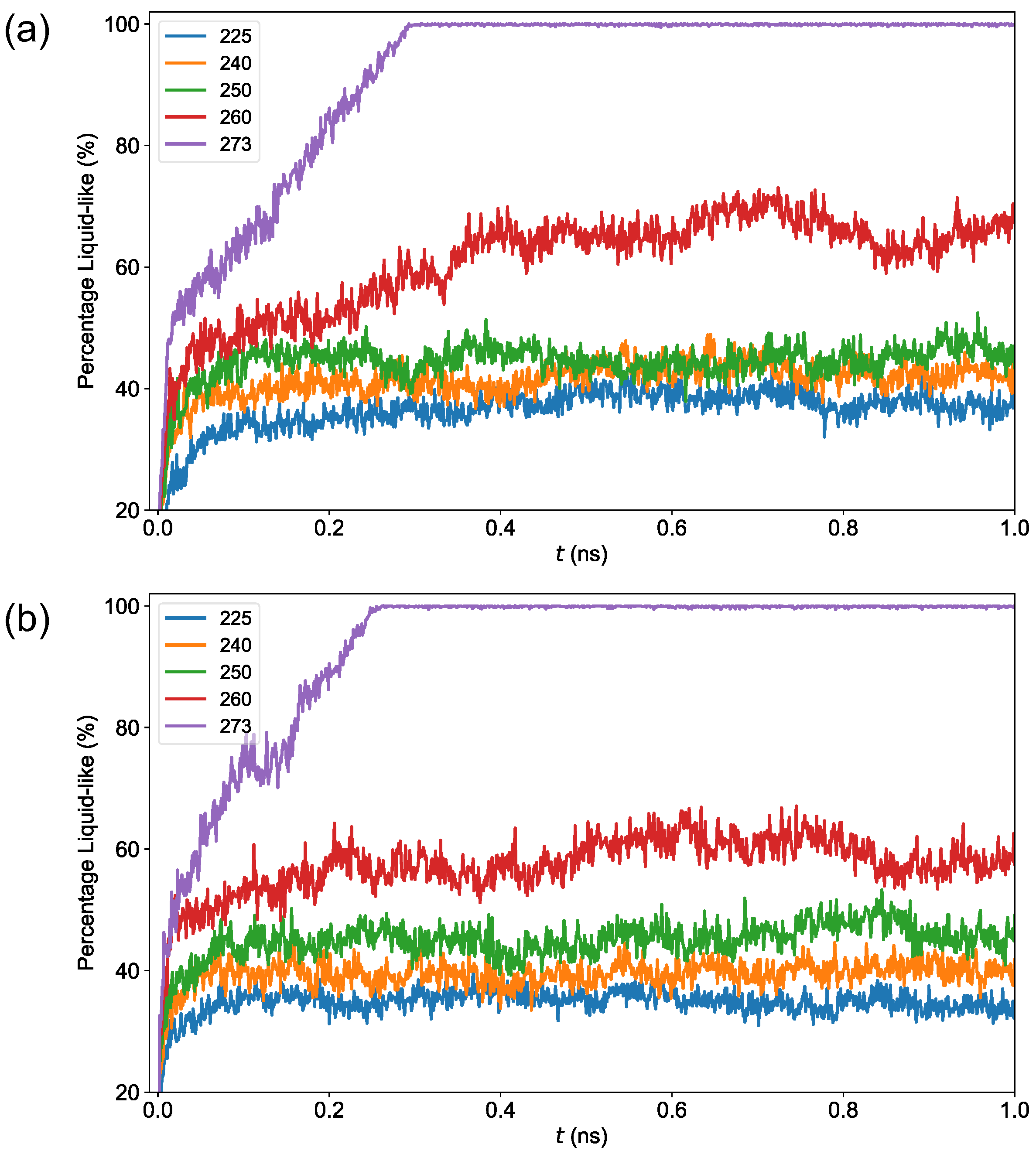
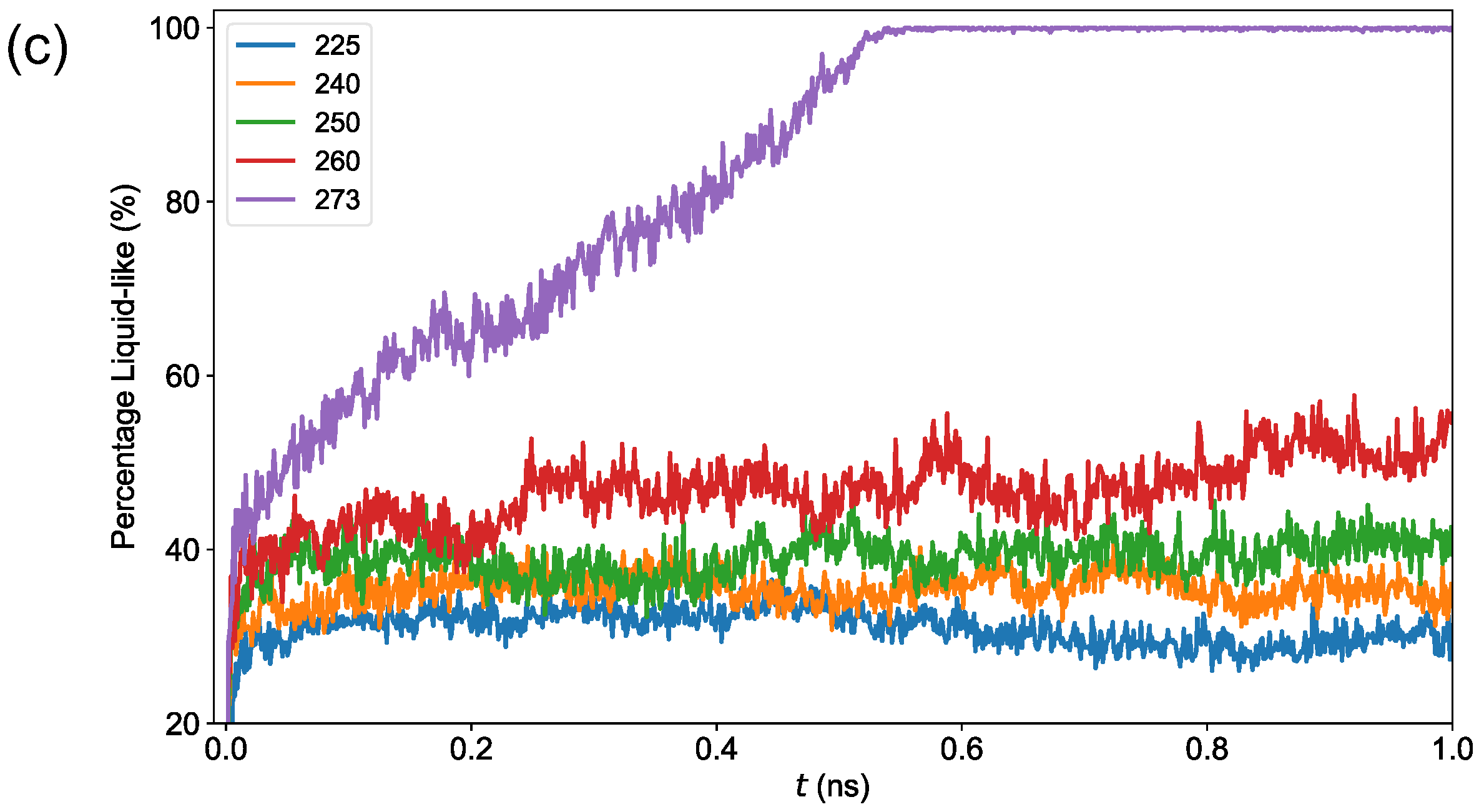
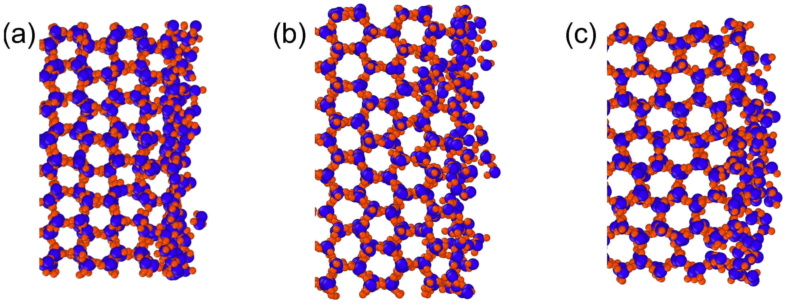
3.2. Premelting Transition

We used the data from the final 100 ps of the 1 ns simulation to obtain stable estimates of the percentage of liquid-like molecules and the density profile. Figure 7 summarizes how the percentage of liquid-like molecules varies with temperature for the primary prismatic, secondary prismatic, and basal facets, respectively. Figure 8 displays the density profiles at various temperatures for these different facets.

As shown in Figure 7, all water molecules become liquid-like when the simulation temperature reaches 273 K, which indicates that complete surface melting happens. However, it is important to note that this is not proof that complete surface melting happens in real physical systems. In fact, experimental evidence on whether complete surface melting occurs at the ice–vapor interface remains inconclusive, with different experiments providing contradictory results [45,46]. The most recent theoretical study by Luengo-Márquez et al. [20], which is based on Lifshitz theory and incorporates dispersion interaction and hydrogen bonding effects, suggests that incomplete surface melting occurs at the melting temperature. The complete melting observed in our simulations may be attributed to the neural network potential’s use of a short cutoff distance of 6.35 Angstroms, which fails to account for the long-range tail of the van der Waals interaction. According to Luengo-Márquez et al. [20], the van der Waals interaction inhibits complete surface melting. This could explain why we observe complete surface melting, as the long-range vdW interaction is not properly accounted for by the potential. Additionally, the size of our simulation box might be too small to make definitive claims about complete or incomplete surface melting.

It is also observed from Figure 7 that the percentage of liquid-like molecules generally differs among the primary prismatic and secondary prismatic. This discrepancy is expected since the hydrogen bonding interactions among water molecules at the interface vary across these three facets, which could affect the width of the premelting layer.

3.3. Dynamic Heterogeneity

We analyzed the dynamical behavior of molecules within the premelting layer at a temperature of 250 K, where a thin premelting layer forms on the primary prismatic, secondary prismatic, and basal facet. Figure 9 shows snapshots of the configurations at 250 K, illustrating the formation of this layer. We specifically focused on the layer on the primary prismatic facet that is located at a distance z greater than 1.2 nm from the center of the bulk ice, the layer on the secondary prismatic facet that is located at a distance z greater than 1.4 nm from the center of bulk, and the layer on the basal facet that is located at a distance z greater than 1.2 nm from the center of bulk. These layers have completely melted, meaning they are entirely composed of liquid-like molecules, as evidenced by the fact that their order parameter q are all less than 0.42, as shown in Figure 10.

The metric we used to quantify the dynamics of the molecules is propensity. Propensity is defined as the squared displacement of a molecule over a given time period, averaged across different trajectories. A detailed definition of this metric can be found in Section 2.5. For our calculations, we used a time period of 100 ps, and the propensity was averaged over 10 different trajectories. Each of these trajectories began from the same initial configuration, which was selected as the final configuration of a preceding 1 ns-long trajectory.

Figure 11 illustrates the propensity of molecules within the premelting layer. The figure reveals regions of high and low mobility. This segregation suggests that the molecules in this liquid layer move collectively, akin to the behavior observed in supercooled liquids [33].

4. Discussion

In this study, we conducted molecular dynamic simulations of the ice–vapor interface at various temperatures across different ice facets. We examined the structural and dynamical properties of the premelting layer. Our results indicate that complete surface melting occurs as the temperature approaches the melting point. Additionally, our simulations reveal that molecules within the premelting layer segregate into clusters of high and low mobility.

We conducted 1 ns-long simulations. The results showed that the percentage of liquid-like water molecules and the density profile number stabilized within 600 ps for all temperatures investigated. However, this does not necessarily indicate full equilibration, as the system may be temporarily trapped in a metastable state. Ensuring complete equilibration would ideally require much longer simulations, potentially on the order of tens of nanoseconds, which are computationally challenging, and while neural network potentials are significantly faster than DFT-based calculations, they are still much more computationally expensive than classical empirical potentials [32]. Future work to optimize the implementation of neural network potentials is necessary to enable simulations on much larger spatial and temporal scales.

Whether complete surface melting happens as the temperature approaches melting temperature has been a long-debated issue. Recent theoretical studies suggest that surface melting remains incomplete at the melting temperature [20]. Our observation of complete surface melting may be due to the fact that the neural network potential used did not account for long-range dispersion interactions. Additionally, the small size of our simulated system might have caused complete surface melting to appear as a finite size artifact. To verify whether complete surface melting truly occurs, simulations should be conducted on much larger systems with long-range dispersion interactions fully taken into account. However, this would require significant simulation time, as current neural network potentials are still more computationally expensive to implement compared to classical potentials, as previously mentioned.

The neural network potential used in our study also missed the long-ranged electrostatic interaction, specifically the tail of the $1/r$ interaction. This is a fundamental limitation of Behler–Parrinello-style neural networks, which apply a cutoff to the symmetry functions and thus fail to capture long-range electrostatic effects. The long-ranged electrostatic interaction significantly affects the orientation of O-H bonds at the interface [28] and may influence the properties of the premelting layer. Recently, several neural network potential models have attempted to incorporate long-ranged electrostatics [28,29,47,48]. In the future, utilizing these enhanced potentials to simulate the ice–vapor interface could be beneficial.

Recently, Bapst et al. [33] used Graph Neural Network to predict the propensity of supercooled liquids based on their initial configurations. In the future, it would be interesting to explore the possibility of using machine learning techniques to predict the propensity of molecules within the premelting layer based on their initial configurations. Additionally, it has been discovered that supercooled liquid consists of both high-density and low-density liquid phases [49,50,51,52,53,54]. Given that the premelting layer exists as a liquid layer at low temperatures, investigating whether it also comprises high-density and low-density phases would be intriguing. However, verifying this would require simulations on a much larger spatial and temporal scale than those conducted in this study.

All simulations in this work are conducted in the NVT ensemble, with the size of the simulation box remaining fixed as the simulation temperature varies. Since the crystal is in contact with vapor along the z-direction, the z component of the crystal’s pressure remains close to zero. However, the x and y components of the pressure are not zero, since the crystal is anisotropic, which may influence premelting behavior. In future studies, implementing proper pressure control to maintain the x and y components of the pressure close to zero would be beneficial.

References

1. Faraday, M. Experimental Researches in Chemistry and Physics; Taylor and Francis: London, UK, 1859. [Google Scholar]
2. Kouchi, A.; Furukawa, Y.; Kuroda, T. X-ray diffraction pattern of quasi-liquid layer on ice crystal surface. J. Phys. Colloq. 1987, 48, C1-675–C1-677. [Google Scholar] [CrossRef]
3. Pluis, B.; Taylor, T.N.; Frenkel, D.; Van Der Veen, J.F. Role of long-range interactions in the melting of a metallic surface. Phys. Rev. B 1989, 40, 1353–1356. [Google Scholar] [CrossRef] [PubMed]
4. Dash, J.G.; Mason, B.L.; Wettlaufer, J.S. Theory of charge and mass transfer in ice-ice collisions. J. Geophys. Res. Atmos. 2001, 106, 20395–20402. [Google Scholar] [CrossRef]
5. Bianco, R.; Hynes, J.T. Heterogeneous Reactions Important in Atmospheric Ozone Depletion: A Theoretical Perspective. Accounts Chem. Res. 2006, 39, 159–165. [Google Scholar] [CrossRef]
6. Abbatt, J.P.D. Interactions of Atmospheric Trace Gases with Ice Surfaces: Adsorption and Reaction. Chem. Rev. 2003, 103, 4783–4800. [Google Scholar] [CrossRef]
7. Conklin, M.H.; Sommerfeld, R.A.; Kay Laird, S.; Villinski, J.E. Sulfur dioxide reactions on ice surfaces: Implications for dry deposition to snow. Atmos. Environment. Part A. Gen. Top. 1993, 27, 159–166. [Google Scholar] [CrossRef]
8. Hudait, A.; Allen, M.T.; Molinero, V. Sink or Swim: Ions and Organics at the Ice-Air Interface. J. Am. Chem. Soc. 2017, 139, 10095–10103. [Google Scholar] [CrossRef]
9. Pickering, I.; Paleico, M.; Sirkin, Y.A.; Scherlis, D.A.; Factorovich, M.H. Grand Canonical Investigation of the Quasi Liquid Layer of Ice: Is It Liquid? J. Phys. Chem. B 2018, 122, 4880–4890. [Google Scholar] [CrossRef]
10. Sazaki, G.; Zepeda, S.; Nakatsubo, S.; Yokomine, M.; Furukawa, Y. Quasi-liquid layers on ice crystal surfaces are made up of two different phases. Proc. Natl. Acad. Sci. USA 2012, 109, 1052–1055. [Google Scholar] [CrossRef] [PubMed]
11. Sazaki, G.; Asakawa, H.; Nagashima, K.; Nakatsubo, S.; Furukawa, Y. How do Quasi-Liquid Layers Emerge from Ice Crystal Surfaces? Cryst. Growth Des. 2013, 13, 1761–1766. [Google Scholar] [CrossRef]
12. Asakawa, H.; Sazaki, G.; Nagashima, K.; Nakatsubo, S.; Furukawa, Y. Prism and Other High-Index Faces of Ice Crystals Exhibit Two Types of Quasi-Liquid Layers. Cryst. Growth Des. 2015, 15, 3339–3344. [Google Scholar] [CrossRef]
13. Murata, K.I.; Asakawa, H.; Nagashima, K.; Furukawa, Y.; Sazaki, G. Thermodynamic origin of surface melting on ice crystals. Proc. Natl. Acad. Sci. USA 2016, 113, E6741–E6748. [Google Scholar] [CrossRef]
14. Dosch, H.; Lied, A.; Bilgram, J. Glancing-angle X-ray scattering studies of the premelting of ice surfaces. Surf. Sci. 1995, 327, 145–164. [Google Scholar] [CrossRef]
15. Bluhm, H.; Ogletree, D.F.; Fadley, C.S.; Hussain, Z.; Salmeron, M. The premelting of ice studied with photoelectron spectroscopy. J. Physics: Condens. Matter 2002, 14, L227–L233. [Google Scholar] [CrossRef]
16. Dash, J.G.; Rempel, A.W.; Wettlaufer, J.S. The physics of premelted ice and its geophysical consequences. Rev. Mod. Phys. 2006, 78, 695–741. [Google Scholar] [CrossRef]
17. Dzyaloshinskii, I.; Lifshitz, E.; Pitaevskii, L. The general theory of van der Waals forces. Adv. Phys. 1961, 10, 165–209. [Google Scholar] [CrossRef]
18. Elbaum, M.; Schick, M. Application of the theory of dispersion forces to the surface melting of ice. Phys. Rev. Lett. 1991, 66, 1713–1716. [Google Scholar] [CrossRef]
19. Limmer, D.T.; Chandler, D. Premelting, fluctuations, and coarse-graining of water-ice interfaces. J. Chem. Phys. 2014, 141, 18C505. [Google Scholar] [CrossRef]
20. Luengo-Márquez, J.; Izquierdo-Ruiz, F.; MacDowell, L.G. Intermolecular forces at ice and water interfaces: Premelting, surface freezing, and regelation. J. Chem. Phys. 2022, 157, 044704. [Google Scholar] [CrossRef] [PubMed]
21. Sibley, D.N.; Llombart, P.; Noya, E.G.; Archer, A.J.; MacDowell, L.G. How ice grows from premelting films and water droplets. Nat. Commun. 2021, 12, 239. [Google Scholar] [CrossRef] [PubMed]
22. Niblett, S.P.; Limmer, D.T. Ion Dissociation Dynamics in an Aqueous Premelting Layer. J. Phys. Chem. B 2021, 125, 2174–2181. [Google Scholar] [CrossRef]
23. Paesani, F.; Voth, G.A. Quantum effects strongly influence the surface premelting of ice. J. Phys. Chem. C 2008, 112, 324–327. [Google Scholar] [CrossRef]
24. Watkins, M.; Pan, D.; Wang, E.G.; Michaelides, A.; Vandevondele, J.; Slater, B. Large variation of vacancy formation energies in the surface of crystalline ice. Nat. Mater. 2011, 10, 794–798. [Google Scholar] [CrossRef]
25. Behler, J. Atom-centered symmetry functions for constructing high-dimensional neural network potentials. J. Chem. Phys. 2011, 134. [Google Scholar] [CrossRef]
26. Behler, J. Four Generations of High-Dimensional Neural Network Potentials. Chem. Rev. 2021, 121, 10037–10072. [Google Scholar] [CrossRef] [PubMed]
27. Zhang, L.; Wang, H.; Car, R.; Weinan, E. Phase Diagram of a Deep Potential Water Model. Phys. Rev. Lett. 2021, 126, 236001. [Google Scholar] [CrossRef]
28. Gao, A.; Remsing, R.C. Self-consistent determination of long-range electrostatics in neural network potentials. Nat. Commun. 2022, 13, 1572. [Google Scholar] [CrossRef]
29. Ko, T.W.; Finkler, J.A.; Goedecker, S.; Behler, J. A fourth-generation high-dimensional neural network potential with accurate electrostatics including non-local charge transfer. Nat. Commun. 2021, 12, 398. [Google Scholar] [CrossRef]
30. Ko, T.W.; Finkler, J.A.; Goedecker, S.; Behler, J. Accurate Fourth-Generation Machine Learning Potentials by Electrostatic Embedding. J. Chem. Theory Comput. 2023, 19, 3567–3579. [Google Scholar] [CrossRef]
31. Deringer, V.L.; Bartók, A.P.; Bernstein, N.; Wilkins, D.M.; Ceriotti, M.; Csányi, G. Gaussian Process Regression for Materials and Molecules. Chem. Rev. 2021, 121, 10073–10141. [Google Scholar] [CrossRef] [PubMed]
32. Mailoa, J.P.; Kornbluth, M.; Batzner, S.; Samsonidze, G.; Lam, S.T.; Vandermause, J.; Ablitt, C.; Molinari, N.; Kozinsky, B. A fast neural network approach for direct covariant forces prediction in complex multi-element extended systems. Nat. Mach. Intell. 2019, 1, 471–479. [Google Scholar] [CrossRef]
33. Bapst, V.; Keck, T.; Grabska-Barwińska, A.; Donner, C.; Cubuk, E.D.; Schoenholz, S.S.; Obika, A.; Nelson, A.W.R.; Back, T.; Hassabis, D.; et al. Unveiling the predictive power of static structure in glassy systems. Nat. Phys. 2020, 16, 448–454. [Google Scholar] [CrossRef]
34. Wohlfahrt, O.; Dellago, C.; Sega, M. Ab initio structure and thermodynamics of the RPBE-D3 water/vapor interface by neural-network molecular dynamics. J. Chem. Phys. 2020, 153, 144710. [Google Scholar] [CrossRef]
35. Morawietz, T.; Singraber, A.; Dellago, C.; Behler, J. How van der waals interactions determine the unique properties of water. Proc. Natl. Acad. Sci. United States Am. 2016, 113, 8368–8373. [Google Scholar] [CrossRef]
36. Hammer, B.; Hansen, L.B.; Nørskov, J.K. Improved adsorption energetics within density-functional theory using revised Perdew-Burke-Ernzerhof functionals. Phys. Rev. B 1999, 59, 7413–7421. [Google Scholar] [CrossRef]
37. Grimme, S.; Antony, J.; Ehrlich, S.; Krieg, H. A consistent and accurate ab initio parametrization of density functional dispersion correction (DFT-D) for the 94 elements H-Pu. J. Chem. Phys. 2010, 132, 154104. [Google Scholar] [CrossRef]
38. Singraber, A.; Behler, J.; Dellago, C. Library-Based LAMMPS Implementation of High-Dimensional Neural Network Potentials. J. Chem. Theory Comput. 2019, 15, 1827–1840. [Google Scholar] [CrossRef]
39. Singraber, A.; Morawietz, T.; Behler, J.; Dellago, C. Parallel Multistream Training of High-Dimensional Neural Network Potentials. J. Chem. Theory Comput. 2019, 15, 3075–3092. [Google Scholar] [CrossRef]
40. Matsumoto, M.; Yagasaki, T.; Tanaka, H. GenIce: Hydrogen-Disordered Ice Generator. J. Comput. Chem. 2018, 39, 61–64. [Google Scholar] [CrossRef] [PubMed]
41. Steinhardt, P.J.; Nelson, D.R.; Ronchetti, M. Bond-orientational order in liquids and glasses. Phys. Rev. B 1983, 28, 784–805. [Google Scholar] [CrossRef]
42. Lechner, W.; Dellago, C. Accurate determination of crystal structures based on averaged local bond order parameters. J. Chem. Phys. 2008, 129, 114707. [Google Scholar] [CrossRef] [PubMed]
43. Widmer-Cooper, A.; Harrowell, P. On the study of collective dynamics in supercooled liquids through the statistics of the isoconfigurational ensemble. J. Chem. Phys. 2007, 126, 154503. [Google Scholar] [CrossRef] [PubMed]
44. Berthier, L.; Jack, R.L. Structure and dynamics of glass formers: Predictability at large length scales. Phys. Rev. E 2007, 76, 041509. [Google Scholar] [CrossRef]
45. Slater, B.; Michaelides, A. Surface premelting of water ice. Nat. Rev. Chem. 2019, 3, 172–188. [Google Scholar] [CrossRef]
46. Li, Y.; Somorjai, G.A. Surface premelting of ice. J. Phys. Chem. C 2007, 111, 9631–9637. [Google Scholar] [CrossRef]
47. Zhang, L.; Wang, H.; Muniz, M.C.; Panagiotopoulos, A.Z.; Car, R.; E, W. A deep potential model with long-range electrostatic interactions. J. Chem. Phys. 2022, 156, 124107. [Google Scholar] [CrossRef]
48. Grisafi, A.; Ceriotti, M. Incorporating long-range physics in atomic-scale machine learning. J. Chem. Phys. 2019, 151, 204105. [Google Scholar] [CrossRef]
49. Debenedetti, P.G.; Sciortino, F.; Zerze, G.H. Second critical point in two realistic models of water. Science 2020, 369, 289–292. [Google Scholar] [CrossRef]
50. Kim, K.H.; Amann-Winkel, K.; Giovambattista, N.; Späh, A.; Perakis, F.; Pathak, H.; Parada, M.L.; Yang, C.; Mariedahl, D.; Eklund, T.; et al. Experimental observation of the liquid–liquid transition in bulk supercooled water under pressure. Science 2020, 370, 978–982. [Google Scholar] [CrossRef]
51. Henry, L.; Mezouar, M.; Garbarino, G.; Sifré, D.; Weck, G.; Datchi, F. Liquid–liquid transition and critical point in sulfur. Nature 2020, 584, 382–386. [Google Scholar] [CrossRef]
52. Brovchenko, I.; Geiger, A.; Oleinikova, A. Liquid-liquid phase transitions in supercooled water studied by computer simulations of various water models. J. Chem. Phys. 2005, 123, 044515. [Google Scholar] [CrossRef] [PubMed]
53. Palmer, J.C.; Martelli, F.; Liu, Y.; Car, R.; Panagiotopoulos, A.Z.; Debenedetti, P.G. Metastable liquid–liquid transition in a molecular model of water. Nature 2014, 510, 385–388. [Google Scholar] [CrossRef] [PubMed]
54. Sastry, S.; Austen Angell, C. Liquid–liquid phase transition in supercooled silicon. Nat. Mater. 2003, 2, 739–743. [Google Scholar] [CrossRef] [PubMed]
Figure 1. A snapshot of the simulation box showing a premelting layer on the primary prismatic facets, viewed through the basal facet. The initial simulation box was generated using GenIce2, with edges aligned perpendicularly to the basal, primary prismatic, and secondary prismatic facets, measuring 2.94143 nm, 3.61461 nm, and 3.12914 nm, respectively. The box was then extended along one edge to a length of 6 nm, while the other two edges retained their original lengths. This extension created a slab structure of vapor, ice, and vapor parallel to the direction of extension.
Crystals 14 00737 g001
Figure 2. (a) The basal, (b) primary prismatic, and (c) secondary prismatic facets.
Crystals 14 00737 g002
Figure 3. Pressure tensor as a function of simulation time. Panel (a) displays the diagonal components of the pressure tensor, while Panel (b) presents the off-diagonal components. The data were collected at 260 K, and correspond to the scenario where the primary prismatic facet is in contact with vapor. The z-direction represents the axis perpendicular to the interface, the x-direction is perpendicular to the secondary prismatic facet, and the y-direction is perpendicular to the basal facet. The time average was performed over a 10 ps interval.
Crystals 14 00737 g003
Figure 4. Distribution of q values obtained from bulk ice and bulk liquid simulations. The bulk ice simulations were conducted at 175 K, and the bulk liquid simulations were performed at 325 K.
Crystals 14 00737 g004
Figure 5. Time evolution of the percentage of liquid-like molecules for different crystal facets at varying temperatures. Panel (a) shows the scenario where the basal facet is exposed to vapor. Panel (b) shows the scenario where the primary prismatic facet is exposed to vapor. Panel (c) shows the scenario where the secondary prismatic facet is exposed to vapor.
Crystals 14 00737 g005aCrystals 14 00737 g005b
Figure 6. Time evolution of the number density profile of oxygen across the interface for different crystal facets at 273 K. Each line in the figure represents a time-averaged result over 100 ps. For example, the legend “0.2–0.3 ns” corresponds to the density profile obtained by averaging the configurations from 0.2 ns to 0.3 ns. Panel (a) shows the scenario where the basal facet is exposed to vapor. Panel (b) depicts the situation with the primary prismatic facet in contact with vapor. Panel (c) illustrates the condition when the secondary prismatic facet is exposed to vapor.
Crystals 14 00737 g006aCrystals 14 00737 g006b
Figure 7. Percentage of liquid-like molecules for different crystal facets at different temperatures. Results are obtained by averaging the data from the final 100 ps of the 1 ns simulation.
Crystals 14 00737 g007
Figure 8. (a) Density profiles at different temperatures across basal, (b) primary prismatic, and (c) secondary prismatic facets. The density profiles are obtained by averaging the data from the final 100 ps of the 1 ns simulation.
Crystals 14 00737 g008
Figure 9. Premelting layer on different facets at 250 K. Panel (a) shows premelting layer on the basal facet observed through the secondary prismatic facet. Panel (b) shows premelting layer on the primary prismatic facet observed through the secondary prismatic facet. Panel (c) shows premelting layer on the secondary prismatic facet observed through the basal facet.
Crystals 14 00737 g009
Figure 10. The order parameter q for the molecules in the premelting layer at 250 K. The blue solid line corresponds to the case when the premelting layer is located on the basal facet, and the range of this layer is defined to be at least 1.2 nm away from the center of the bulk. The orange dashed line corresponds to the case when the premelting layer is located on the primary prismatic facet, and the range of this layer is defined to be at least 1.2 nm away from the center of the bulk. The green dashed line corresponds to the case when the premelting layer is located on the secondary prismatic facet, the range of this layer is defined to be at least 1.4 nm away from the center of the bulk.
Crystals 14 00737 g010
Figure 11. Propensity of premelting layer at different facets. The brightness of the color of each particle indicates its propensity. The brighter the colorer, the larger the prorensity. The colorbar unit is nm2. (a) Propensity of molecules within the premelting layer on the basal facet. (b) Propensity of molecules within the premelting layer on the primary prismatic facet. (c) Propensity of molecules within the premelting layer on the secondary prismatic facet.
Crystals 14 00737 g011
Disclaimer/Publisher’s Note: The statements, opinions and data contained in all publications are solely those of the individual author(s) and contributor(s) and not of MDPI and/or the editor(s). MDPI and/or the editor(s) disclaim responsibility for any injury to people or property resulting from any ideas, methods, instructions or products referred to in the content.