3.1. Edge Dislocation Structure
The shortest perfect Burgers vector in an hcp lattice is
, and the most common dislocation slip planes are the basal,
, and prism,
, planes [
2,
12,
25]. The preference of the glide plane is determined by the energy and stability of a stacking fault. If a low-energy metastable stacking fault with vector
exists,
, then the dislocation normally dissociates in the basal plane into two Shockley partial dislocations bounding a ribbon of fcc-like stacking fault [
2,
12,
25]. Such a dissociation process is described in crystallographic notation as:
The resulting system geometry generally consists of two partial dislocations lying on the basal plane at
of the initial Burgers vector
(or
, if referred to the dislocation line) and with partial Burgers vectors
.
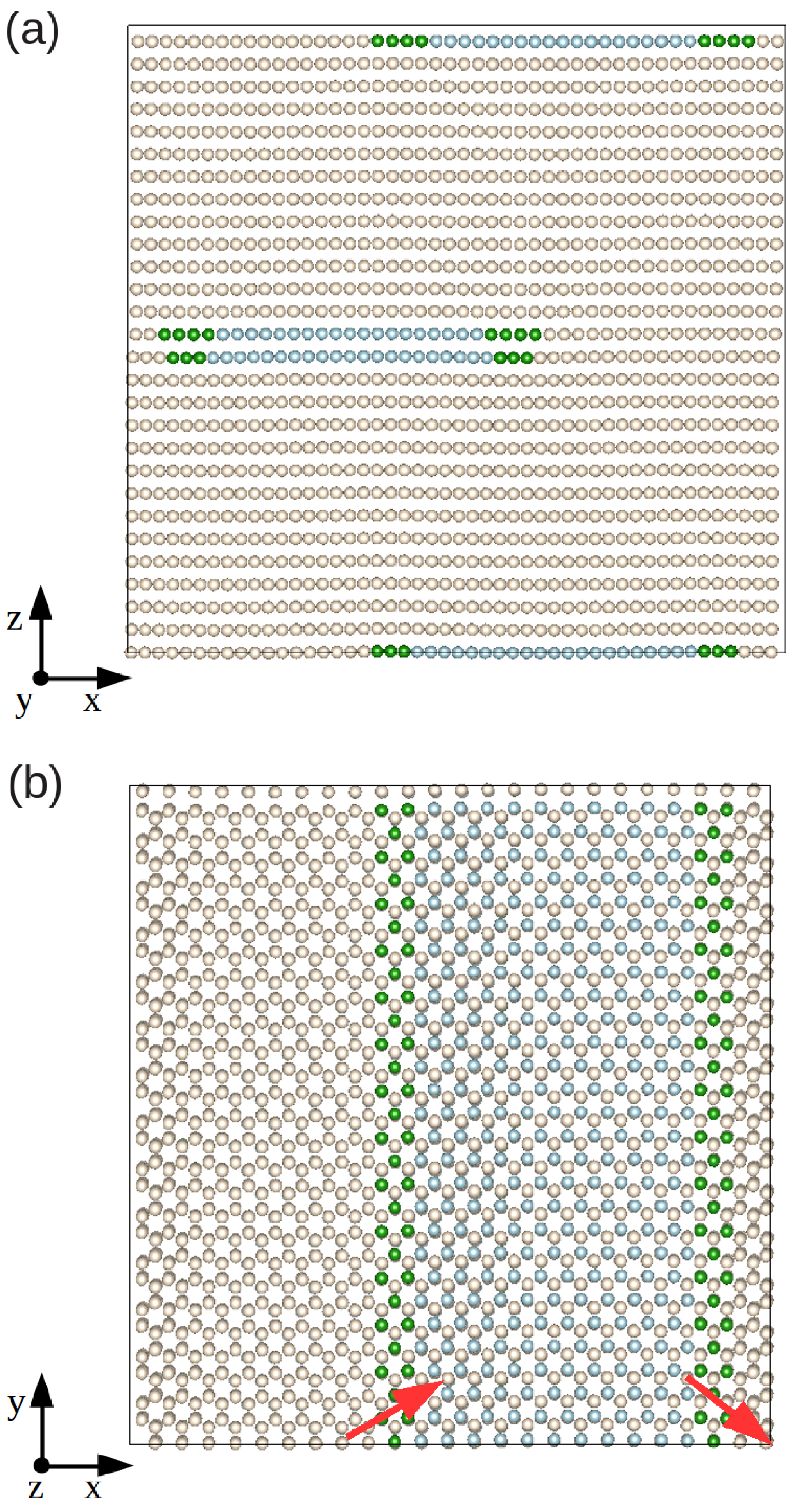
In
Figure 1a,b, we represent the final relaxed configuration of our model hcp Xe solid in which we initially created an edge dislocation with its line oriented along the
y-direction. The full relaxation was performed via minimization of all the atomic forces,
, and mechanical stresses,
(see
Section 2.1). By using the CNA analysis method (see
Section 2.2.3), we are able to distinguish the atoms that belong to the dislocation core (green) or to the fcc-like stacking fault (blue), and those that render the usual hcp ordering (yellow). The relaxed structure clearly shows two Shockley partial dislocations oriented as
and
with respect to the initial Burgers vector
, and a ribbon of fcc-like stacking fault between them; we note that the same structural behavior is observed also in classical metallic (e.g., Zr [
2,
12]) and quantum rare-gas (e.g.,
He [
11]) hcp crystals.
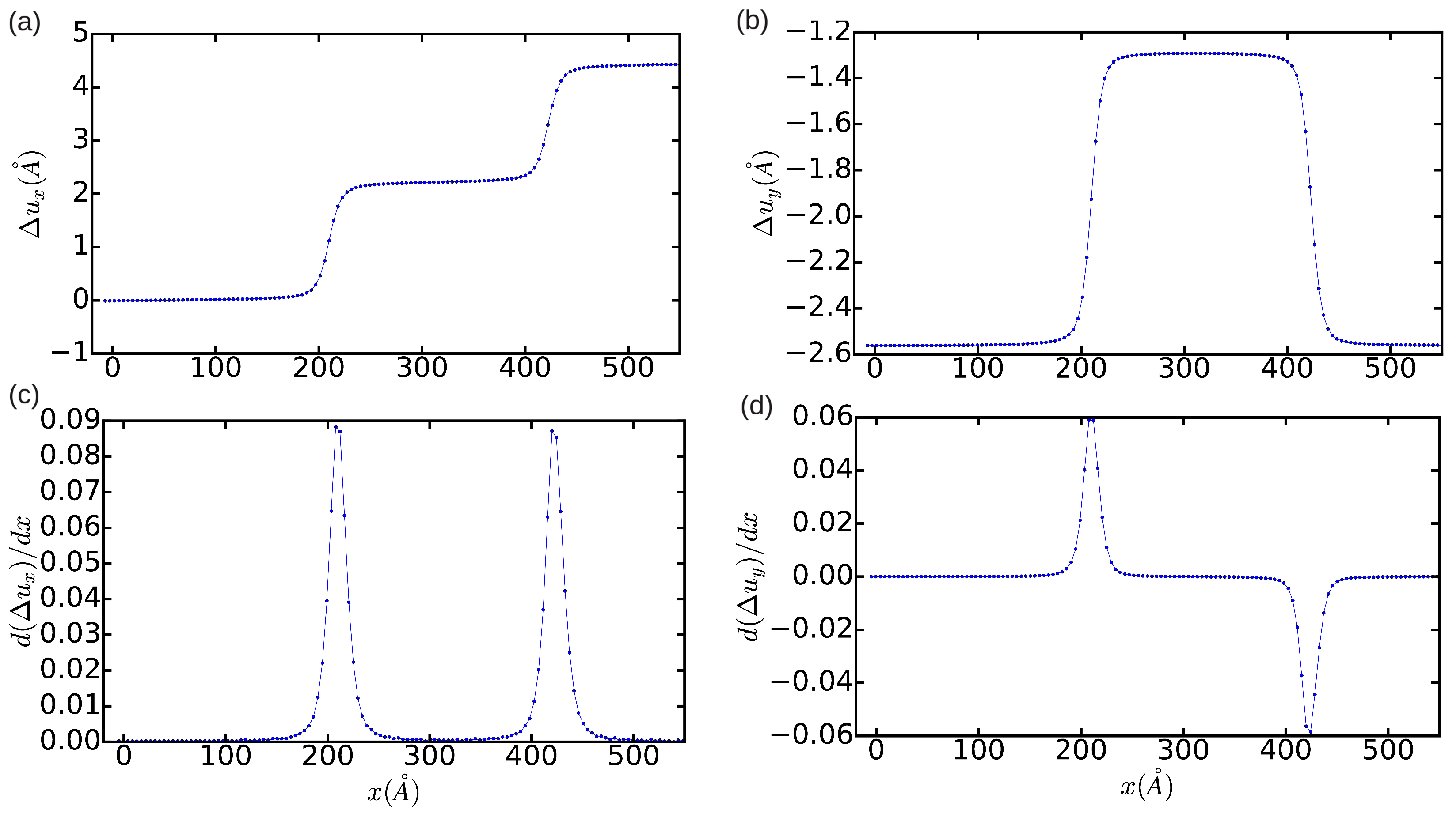
In order to provide a quantitative description of the relaxed dislocation configuration, we employed the differential displacement (DD) analysis method (
Section 2.2.1). In
Figure 2a,b, we plot the relative displacement of the atoms delimiting the glide plane, and, in
Figure 2c,d, the corresponding partial Burgers vector components
. It is shown that, as expected, integration of
and
along the
x-direction leads to non-zero edge and null screw total dislocation components, respectively. The width of the resulting fcc-like stacking fault,
, as deduced from the distance between the two maxima in
Figure 2c, is approximately equal to
. The width of the dislocation core, which can be defined as the region in which the atomic disregistry is greater than the half of its maximum, is found to be ∼12.5
a. This latter quantity has an unusually large value, which indicates the presence of very mobile dislocations (we will comment again in this point in
Section 3.3).
Concerning the technical aspects involved in the simulation of dislocations, we have analyzed the effects of reducing the size of the simulation cell on the determination of the final equilibrium state. This type of analysis is especially useful for interpreting the results obtained in quantum and first-principles simulations where, due to the high computational expense involved, one only can handle systems made up of few hundreds or thousands of atoms [
11,
26].
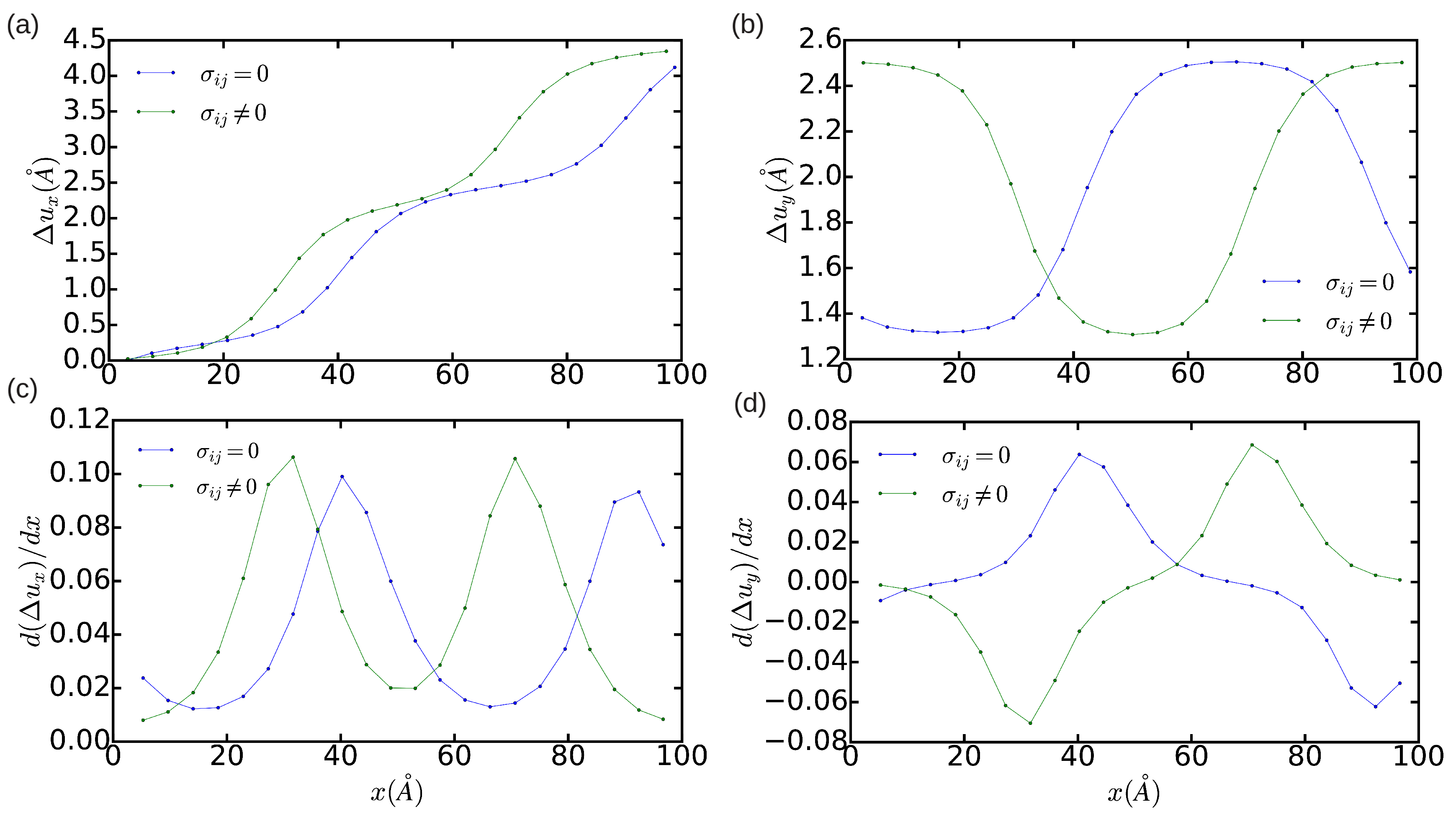
Figure 3 and
Figure 4 show the DD analysis performed in two simulation cells containing 18,424 and 1368 atoms, respectively. In the
n = 18,424 case, we have also analyzed the effects of constraining the shape of the simulation cell to orthorhombic, that is, of not relaxing it (hence
). In
Figure 3a–d (blue lines), it is appreciated that
now is equal to
and the width of the dislocation core is ∼5
a. These values are significantly smaller than the results obtained in the simulation cell containing 344,544 atoms, which in principle are not affected by finite-size errors. Nevertheless, integration of the corresponding
and
partial Burgers vector components along the
x direction still provides non-zero edge and null screw total dislocation components, and the two Shockley partial dislocations can be clearly differentiated in the DD plots shown in
Figure 3. Meanwhile, it is found that when the shear stresses on the simulation cell are not minimized the separation between the two partial dislocations reduces to approximately
. In addition, the orientation of the two partial dislocations changes from
and
to
and
, as compared to the minimum-energy case
. Nevertheless, it may be reasonably concluded that, in the particular case of simulating edge dislocations, the inaccuracies deriving from the use of relatively small orthorhombic boxes containing up to ∼
atoms are not critical. In the
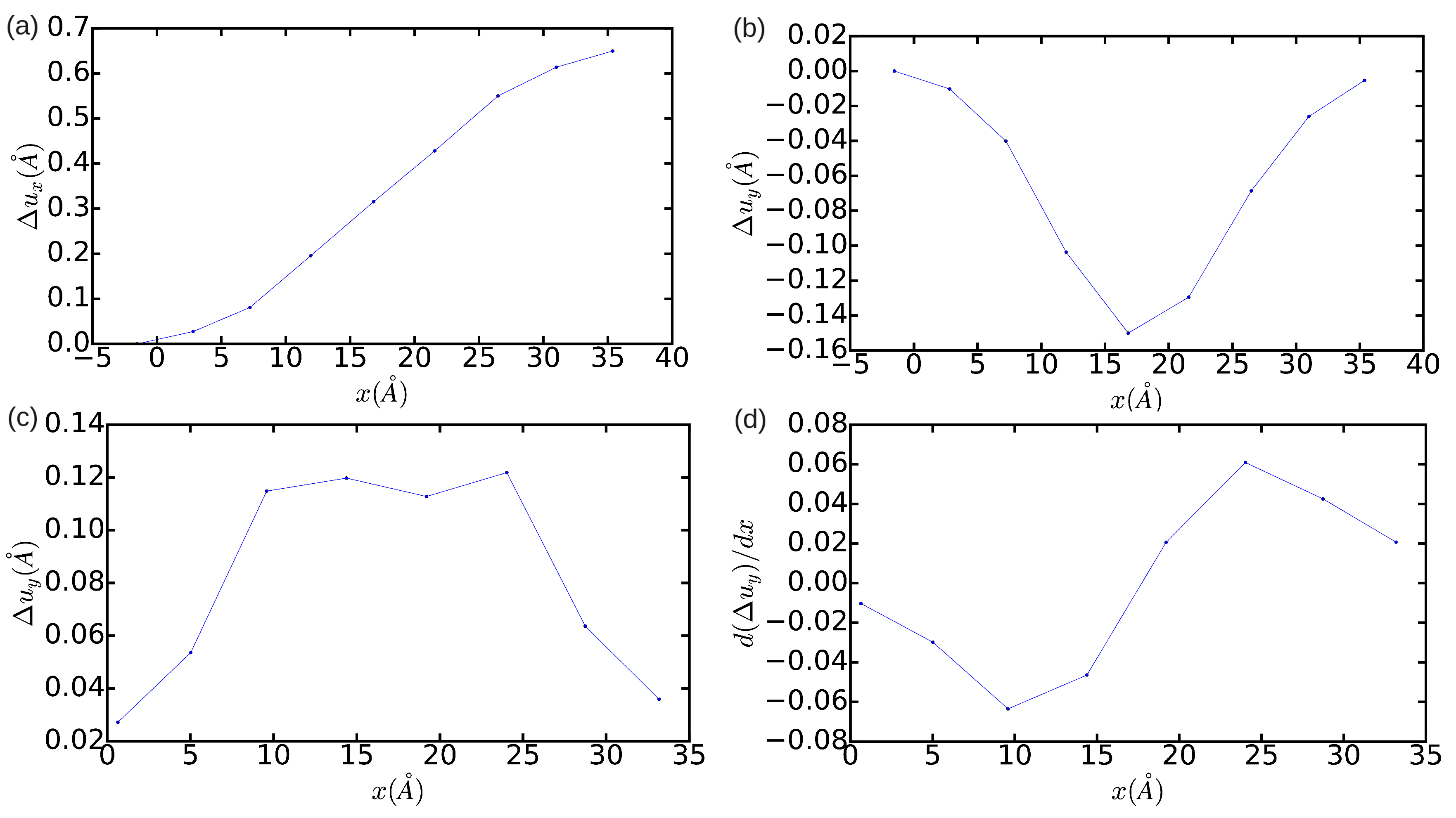
case (see
Figure 4), by contrast, it is found that the edge dislocation hardly can get dissociated owing to the limited size of the simulation cell, which artificially prevents the appearance of any stacking fault (that is, only one diffuse maximum is appreciated in
Figure 4c). Moreover, integration of the
partial Burgers vector component along the
x-direction neither provides an exact null value for the total screw dislocation component (see
Figure 4d). In view of the results enclosed in
Figure 2,
Figure 3 and
Figure 4, we may conclude that the use of small simulation cells containing just up to ∼1000 atoms is likely to produce unrealistic dislocation configurations (see, for instance, Ref. [
26]).
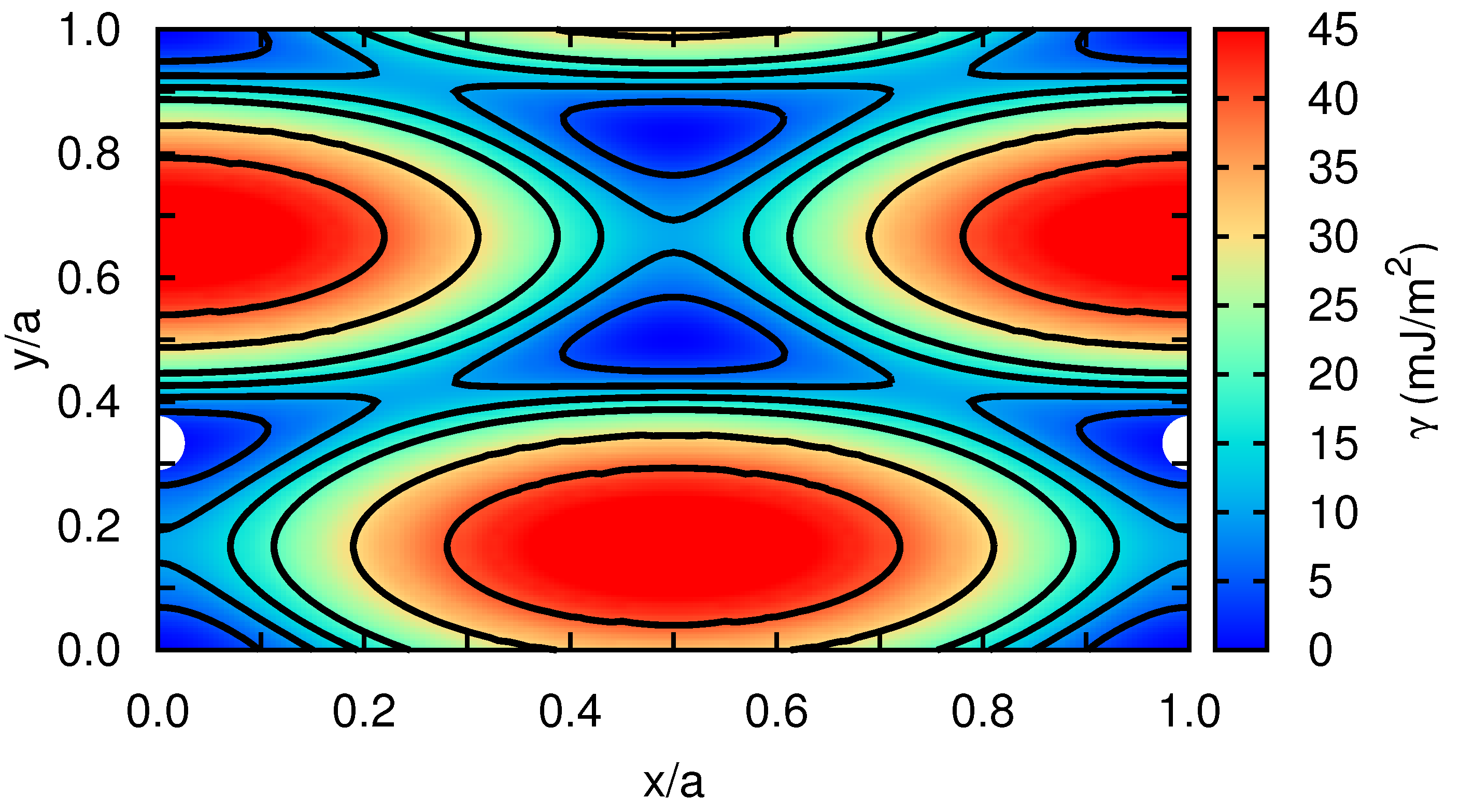
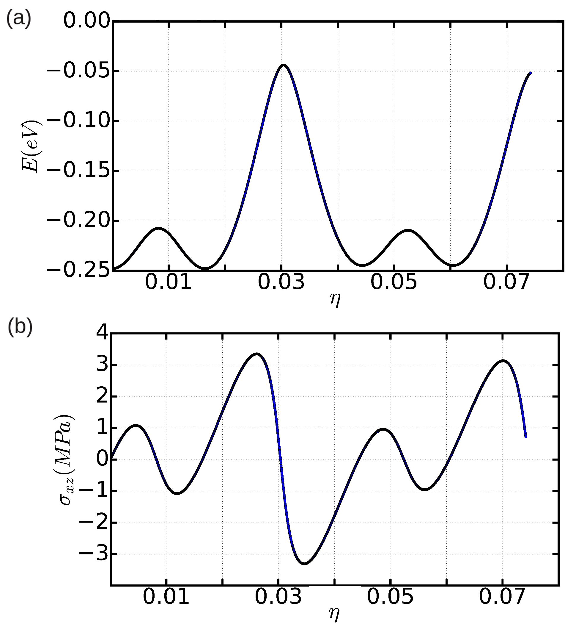
In order to get quantitative insight into the metastable stacking fault that induces the dissociation of the edge dislocation into Shockley partials within the basal plane, we have computed the stacking fault energy in our model hcp crystal as a function of the fault plane displacement,
[
12]. For this calculation, first we rigidly displace one half of the crystal with respect to the other over a grid of
points spanning all possible faults within the
x–
y plane. Subsequently, at each
point, the atoms are allowed to relax perpendicular to the fault plane, which is along the
z-direction, by potential energy minimization (i.e., zero-temperature conditions are assumed). Our simulation cell contains a total of 8100 Xe atoms, and we apply periodic boundary conditions over the
x–
y fault plane and rigid boundary conditions along
z. Our stacking fault energy results are represented in
Figure 5, for which a spline-based interpolation has been used in order to provide smooth iso-
contours. We actually find a metastable stacking fault at
, which is
, similarly to what has been reported by other authors for classical hcp metals [
12]. According to our calculations, the energy of the
stacking fault,
, is equal to
mJ/m
. (It is worth noting that the numerical accuracy in our
estimations is below
mJ/m
.) We also calculated the energy of the metastable stacking fault associated to an edge dislocation with its line laying on the hcp prism plane (see, for instance, Figure 2b in Ref. [
12]). In that case, we obtained a
value of 15 mJ/m
, which is about three orders of magnitude larger than the value calculated for the basal plane. This result shows a major tendency towards dislocation dissociation into Shockley partials in the basal plane.
As expected, the
values calculated in Xe turn out to be extremely small as compared to those obtained in other hcp crystals where the interactions between atoms are much stronger (e.g.,
mJ/m
in Zr [
12,
27,
28]). We note that Keyse and Venables already measured more than 30 years ago the stacking fault energy in fcc Xe at low temperatures by means of transmission electron microscopy techniques [
29]. In particular, they found a
value of
mJ/m
at a temperature of
K, which is about two (one) orders of magnitude larger (smaller) than the stacking fault energy that we have determined for the basal (prism) plane in the hcp phase. The reasons behind these discrepancies may be possibly understood in terms of the different crystal structure considered in our calculations and also of likely inaccuracies present in the employed interaction pairwise potential.
Once the metastable stacking fault energy is known, we can estimate from elastic theory the expected equilibrium distance between the Shockley partial dislocations, which is the width of the resulting fcc-like stacking fault, with the formula [
1,
2]:
where likely elastic anisotropic effects have been disregarded,
G represents the shear modulus of the system (which we estimate here to be 200 MPa), and
the modulus of the corresponding partial Burgers vector. By performing the necessary numerical substitutions, we find that in the basal plane
is equal to
. We recall that, in the larger simulation cell considered in this study, we have found that
approximately amounts to
(see
Figure 2c,d), which turns out to be of the same order of magnitude and larger than
. Consequently, the results obtained in the 344,544-atoms system may be considered to be virtually free of finite-size bias.
Recently, Landinez-Borda et al. have estimated an almost vanishing
value of
mJ/m
in solid
He at ultralow temperatures by using quantum Monte Carlo simulation techniques [
11]. In an attempt to quantify the importance of quantum nuclear effects on the stacking fault energy of solid helium, we have performed analogous classical
calculations to those described for Xe but considering the same volume conditions, interatomic interactions, and atomic mass than in Ref. [
11]. Our classical calculations in solid
He render a stacking fault energy of
mJ/m
, which is orders of magnitude smaller than the value estimated in solid Xe. By comparing this result to the stacking fault energy calculated by Landinez-Borda et al., we may conclude that quantum nuclear effects are responsible for a
reduction of the ∼30% . Consequently, quantum nuclear fluctuations further contribute to the dissociation of edge dislocations into partials in solid
He and probably also in any other quantum crystal (e.g., H
, Ne and LiH [
5,
30,
31]).
3.3. Dislocation Mobility: Finite-T Simulations
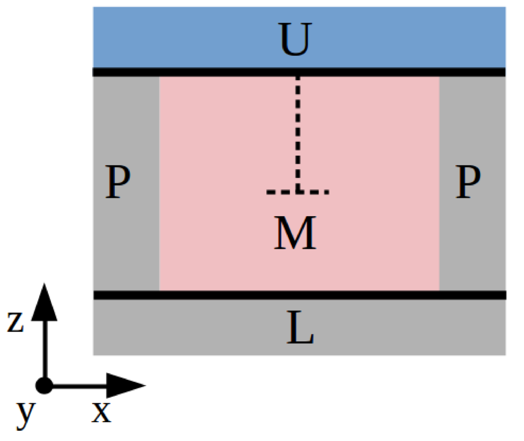
We have estimated the basal mobility of an edge dislocation in our model hcp rare-gas solid at
conditions by performing molecular dynamics (MD) simulations in a simulation cell containing
n = 18,424 atoms. Fully periodic boundary conditions are employed and a
z-vacuum slab is introduced in order to avoid the presence of additional dislocations in the upper and lower edges of the simulation cell (which otherwise would interact with the principal dislocation). No external stresses are considered in our MD simulations, which are performed in the canonical,
, microcanonical,
, and isothermal-isobaric,
ensembles. For the cases in which the volume is fixed, we use the simulation cell obtained through full geometry relaxation of the system. Likewise, the pressure is set to zero in the
calculations [
17]. All simulations are performed with a time step of
ps and last for a total of 800 ps. The position of the (dissociated) edge dislocation is monitored with three different methods: the differential displacement (DD,
Section 2.2.1), the nearest neighbor (NN,
Section 2.2.2), and the common neighbor (CNA,
Section 2.2.3). In the DD case, due to the high sensitivity of this method to thermal fluctuations, we have averaged the positions of the atoms over five consecutive time steps. In the NN case, for the sake of simplicity, we have averaged the position of the atoms with nearest neighbor number different from 12, hence we have determined the center position of the stacking fault; we note that the NN method provides inaccurate results in the
simulations owing to the fluctuations of the simulation cell, thus that particular case must be disregarded in what follows (shown here just for completitude).
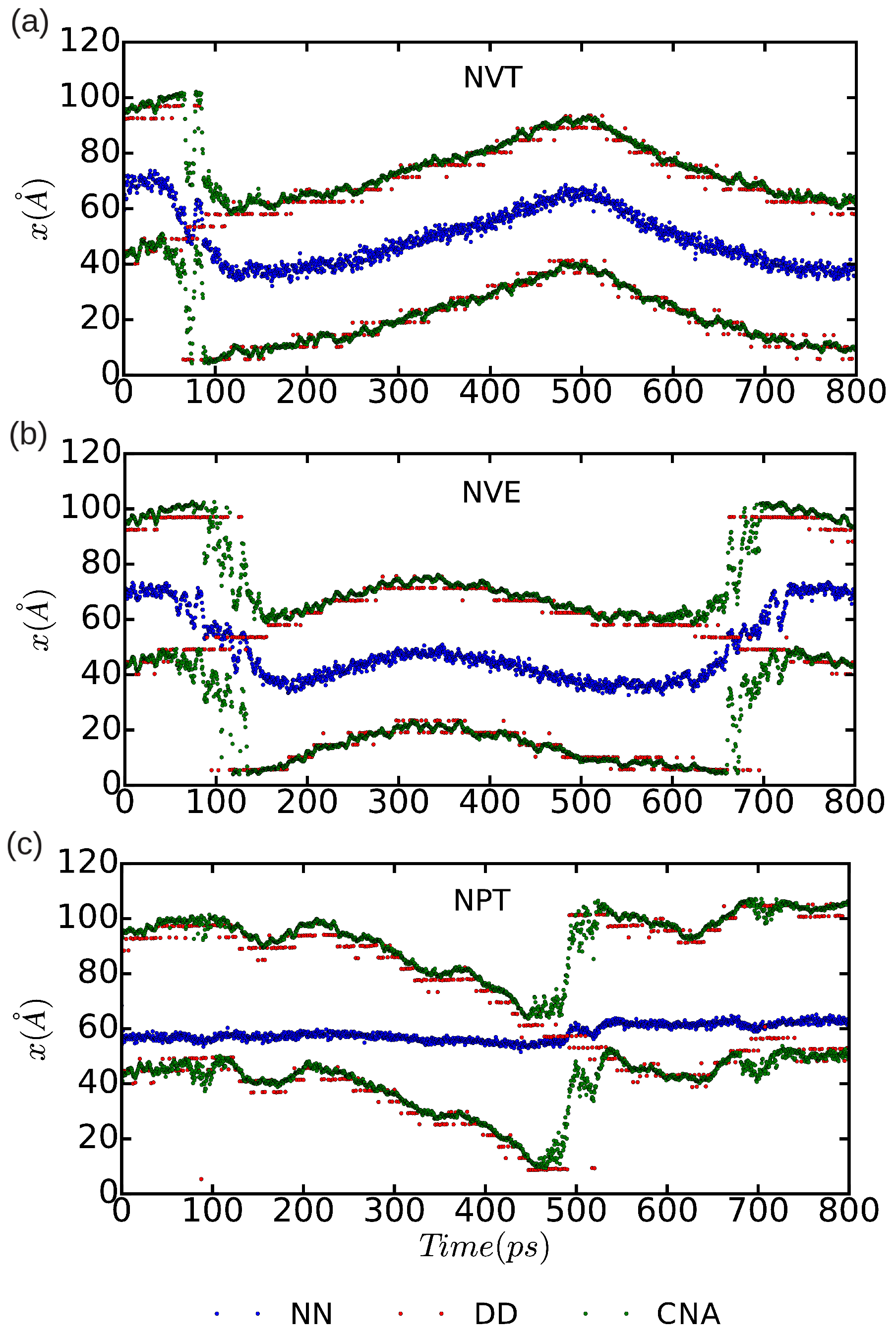
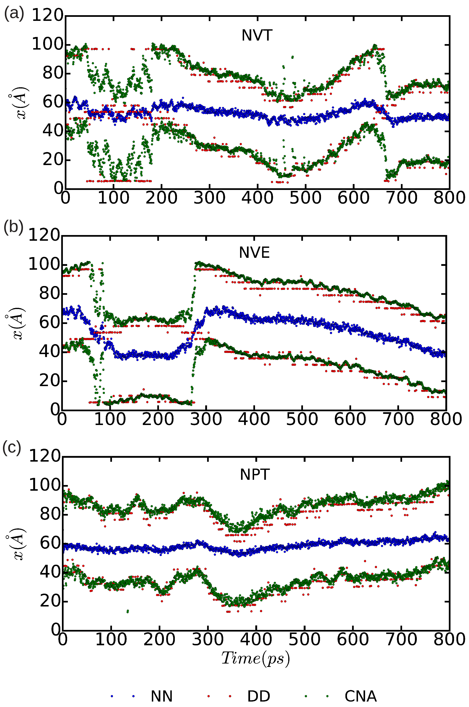
In
Figure 10 and
Figure 11, we represent the position of the (dissociated) edge dislocation expressed as a function of time at a temperature of 25 and 50 K, respectively. It is appreciated that, in spite of the absence of shear stresses, the dislocation moves at temperatures as low as 25 K, which are well below the corresponding Debye temperature (
K [
16]). (Cautiously, we have monitored the size of the fluctuating stresses in our MD simulations, which are null in average, and checked that in fact they are not responsible for the observed dislocation glide (e.g.,
fluctuations
in the
runs). The partial dislocations move either to the left or to the right along the
x-direction with equal probability, which is fully consistent with the absence of applied stresses. In our MD simulations, the partial dislocations practically remain rigid along the
y-direction as no kinks or jogs are observed along their dislocation lines (although for a more detailed analysis of the structural properties of the mobile dislocations the dimensions of our simulation cell should probably need to be increased). It is worth noting that, in the
simulations, we have selected
and assigned initial velocities to the atoms reproducing the temperatures chosen in the
and
runs; consequently, after initializing the
simulations, half of the total kinetic energy is transformed into potential and the effective temperature of the system is halved (i.e.,
and 25 K, respectively). In spite of such a reduction in temperature, one still can observe in
Figure 9b that the dislocation remains mobile in the
simulations. These results clearly make evident a very low resistance of the rare-gas lattice to dislocation glide. From
Figure 10 and
Figure 11 we can also estimate the width of the fcc-like stacking fault in our MD simulations,
, which corresponds to the position difference between the two dislocation cores. We enclose our averaged
results in
Table 1, expressed as a function of temperature and simulation ensemble. It is appreciated that all three ensembles provide consistent results and that, as expected, thermal excitations tend to increase the
fluctuations.
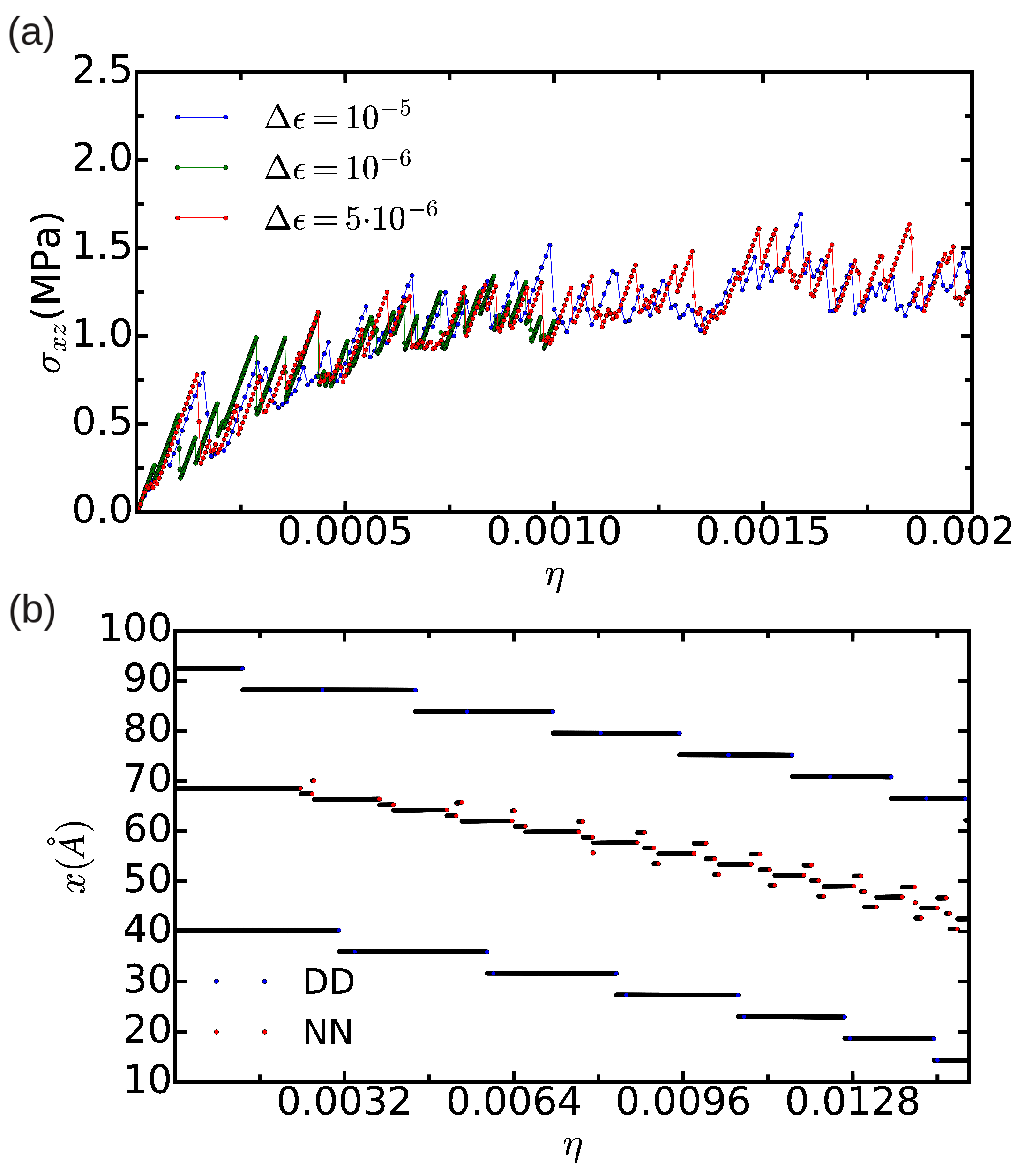
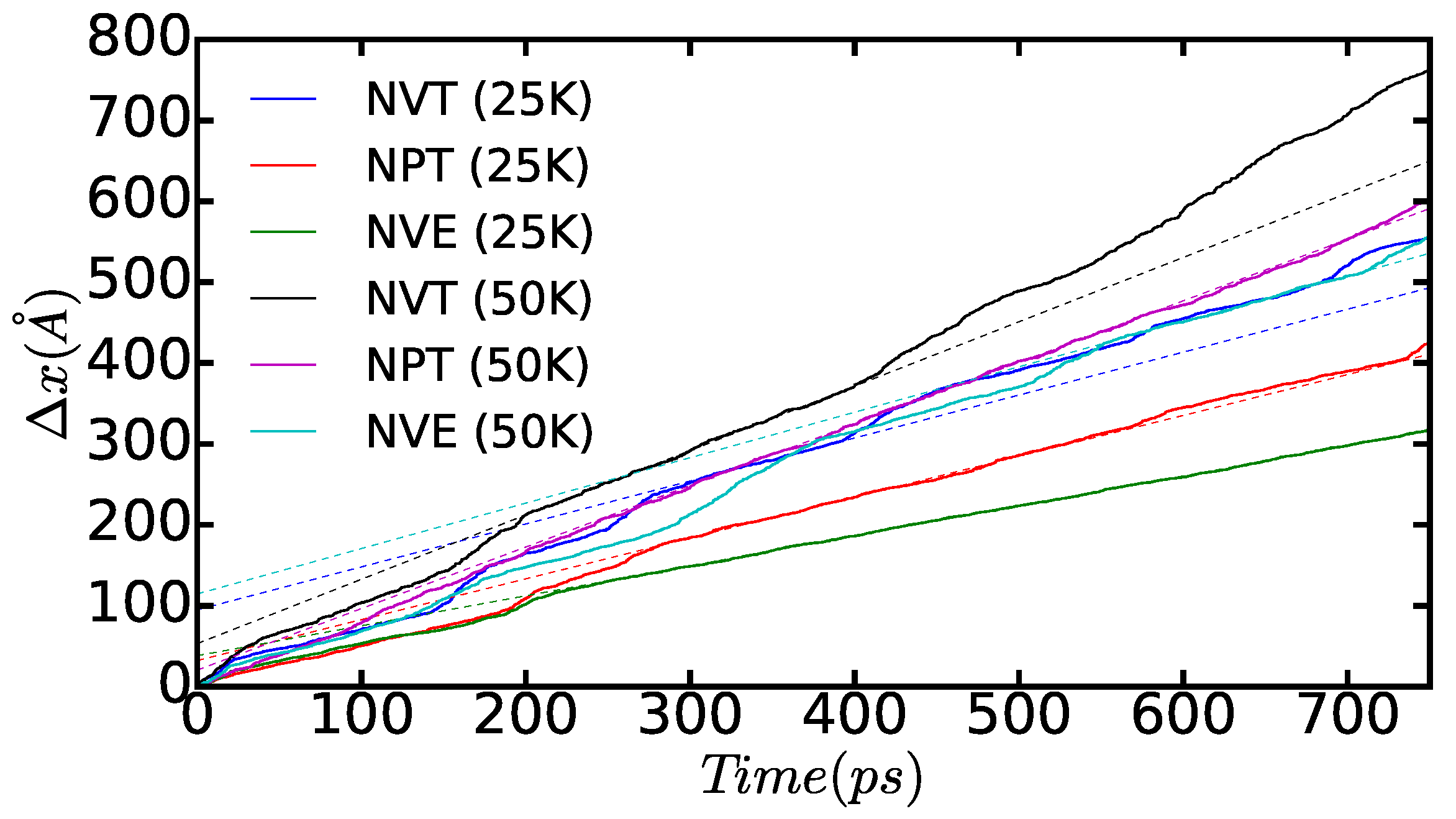
In
Figure 12, we show the time-accumulated average displacement of the dissociated edge dislocations,
, expressed as a function of time, temperature, and simulation ensemble. In particular, we calculate this quantity with the formula:
where
corresponds to the average position of the atoms belonging to the dislocations along the
x direction at time
t (that is, as shown in
Figure 10 and
Figure 11) and
is equal to a time step in our molecular dynamic simulations. A series of kinks appear in the figure that are a consequence of the dislocation cores passing through the boundaries of the simulation cell (that is, due to use of periodic boundary conditions during the crossing of an edge, some of the atoms belonging to the same dislocation core are located in one extreme of the box, whereas the rest remain in the opposite boundary). From the slope of the linear fits to the
data points, which are not affected by such a periodic boundary
artifact, we can deduce the module of the average diffusion velocity of the dislocations,
, as a function of temperature and simulated thermodynamic ensemble. The results enclosed in
Table 1 show that simulations performed both in the
and
ensembles render very similar
values; by contrast, simulations performed in the
ensemble systematically provide smaller dislocation diffusion velocities due to the effective reduction in the temperature of the system (see preceding paragraph). Interestingly, our MD results suggest a square root-like dependence of
on temperature,
. For instance, in the
and
cases, we realize that
, and, when comparing those results with the values obtained in the
ensemble, we consistently find that
. This behavior appears to depart significantly from the Arrhenius-like relation that is expected for thermally activated dislocations, namely
, and which has been observed in other materials at high temperatures [
2,
40,
41].
It is physically insightful to compare the
values obtained in our model rare-gas solid with those reported for other materials with the hcp structure. In the case of Zr, Khater and Bacon have estimated edge dislocation velocities within the basal plane of about 100 ms
at room temperature and practically vanishing applied shear stresses (see Figure 7a in Ref. [
12]). In the present case, similar
values are obtained already at a much lower temperature of 50 K and nominally zero mechanical stress. This comparison comes to show that edge dislocations in classical hcp rare-gas solids are much more mobile than in structurally analogous metals. The origins of such differences may reside on the interatomic interactions (mind that the atomic masses of Zr and Xe atoms are roughly comparable), which in the case of rare gases are extremely weak [
33].


