1. Introduction
Despite the existence of good physical methods for phasing the X-ray reflections of a protein crystal, direct phasing remains a challenging theoretical problem. Iterative projection algorithms have been widely used for phase retrieval [
1,
2,
3,
4,
5,
6,
7,
8,
9,
10,
11,
12,
13,
14,
15,
16,
17].
For crystals with high solvent content or with adequate non-crystallographic symmetry (NCS), it has been demonstrated that direct phasing is possible [
10,
12,
13]. Completely
ab initio phasing using an iterative algorithm has been reported [
13]. A crucial component of the algorithm is the hybrid-input-output (HIO) scheme employed in enforcing the solvent constraint [
1,
2,
3]. Instead of requiring the solvent density to be strictly constant, the HIO method uses a negative feedback mechanism to gradually modify the solvent density so that it tends to become more constant.
It has been argued that for HIO to work properly, oversampling is required [
5]. For a given number of protein atoms, availability of higher resolution data would therefore seem more favorable. It turns out that the oversampling condition is independent of the resolution and depends only on the structural redundancy [
5,
11,
13], i.e., the low- and medium-resolution data are sufficient for the determination of the corresponding phases as long as there is enough redundancy (high solvent content or NCS).
Ab initio phasing at very low resolution has been reported with a generalized likelihood based approach [
18,
19]. In this paper, we describe a series of trial calculations using the HIO algorithm involving data at various resolutions (from 2.85 Å to 7 Å). At each resolution, the HIO method is capable of yielding useful structural information. As expected, only 3.5 Å or higher resolution data can lead to atomic modeling. In addition, at lower resolution partial information such as the secondary structures or the protein boundary can still be obtained.
Membrane protein crystals usually have large solvent content and do not diffract to high resolution. It could be challenging to retrieve the phase using conventional methods [
20]. The results of our trial calculations indicate a potential new phasing approach for membrane proteins.
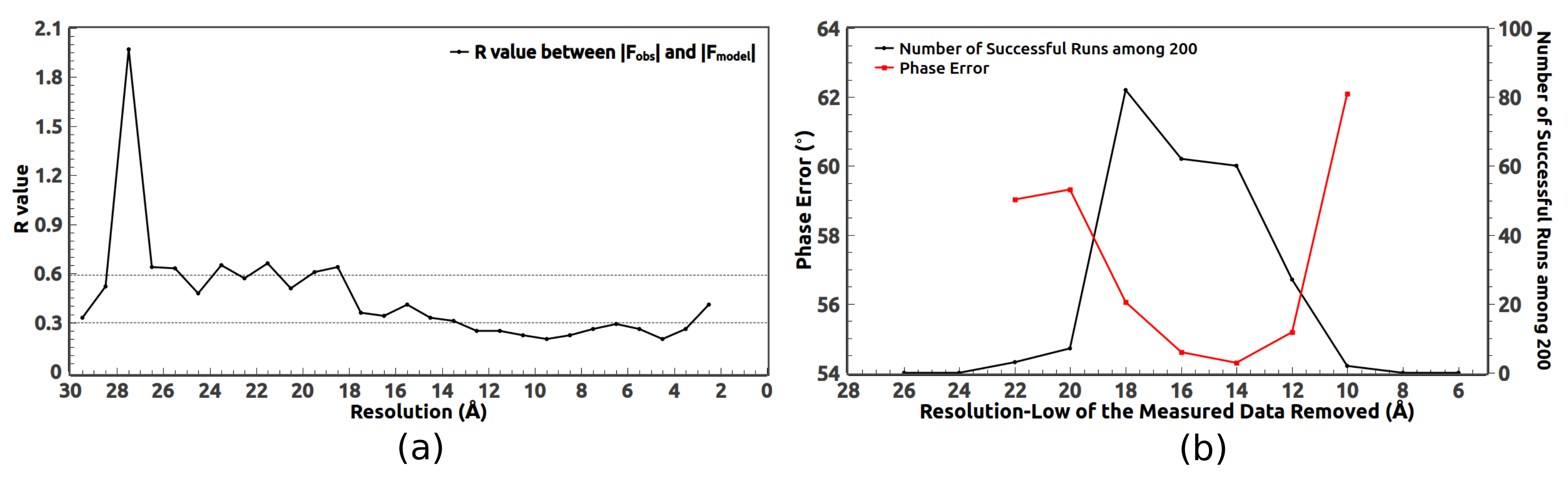
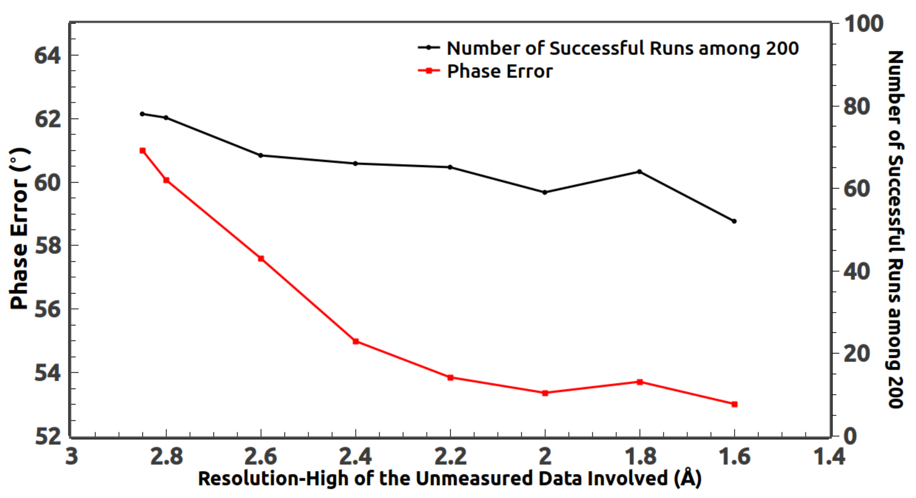
When collecting the experimental data, some low-resolution reflections are missing due to the beam stop. Those measured low-resolution reflections with very small diffraction angles are usually not accurate and deviate a lot from their expected values. They should be replaced by the calculated values during the phasing process. At the same time, we find the HIO phasing method benefits from including some unmeasured high-resolution reflections [
21,
22,
23,
24]. This is because using the calculated values of those reflections makes the computed density in real space more smooth.
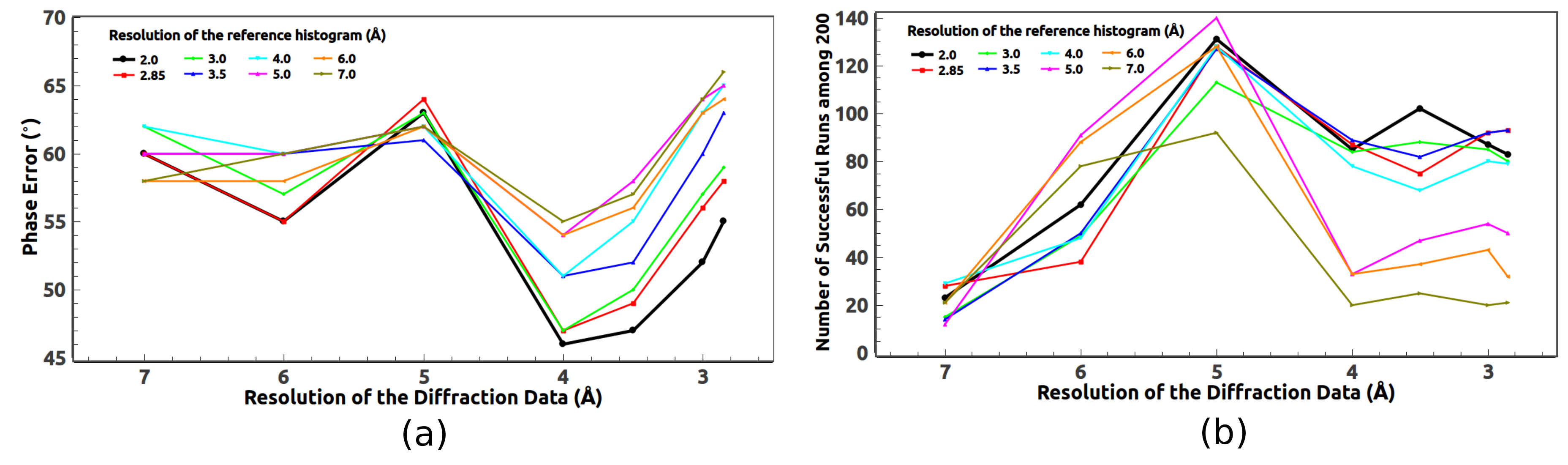
Another resolution dependence of the direct phasing method is histogram matching. A reference histogram is well-known to be very helpful for density modification inside the protein region [
25,
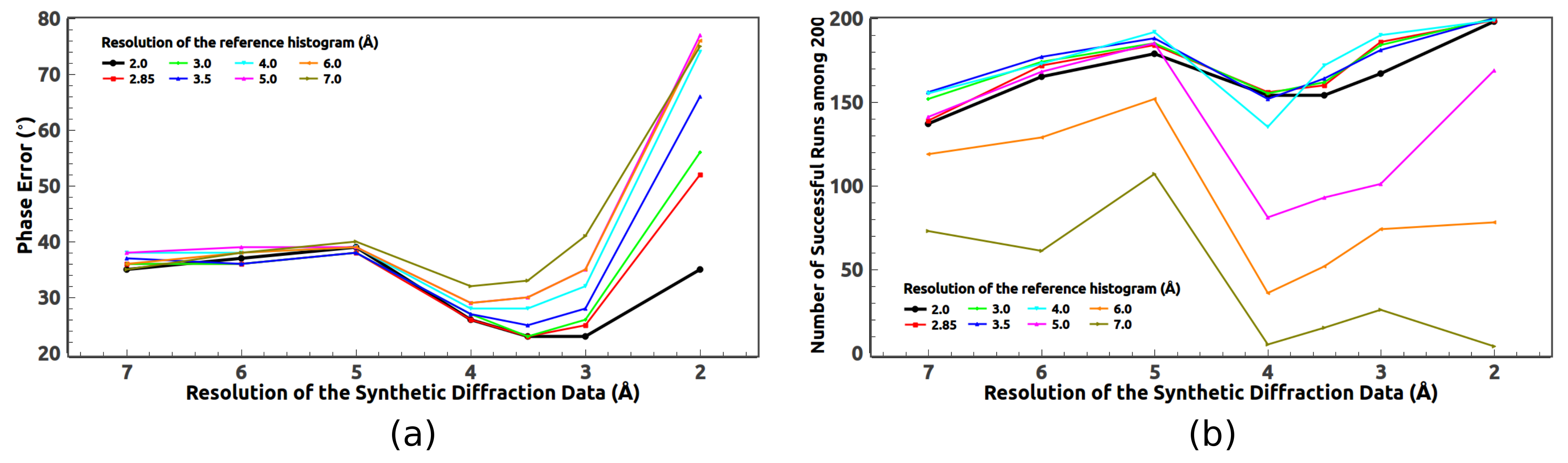
26]. It is also very much resolution dependent. It would seem only natural that the resolution of the reference histogram should match that of the diffraction data. However, trial calculations show that is not always the case.
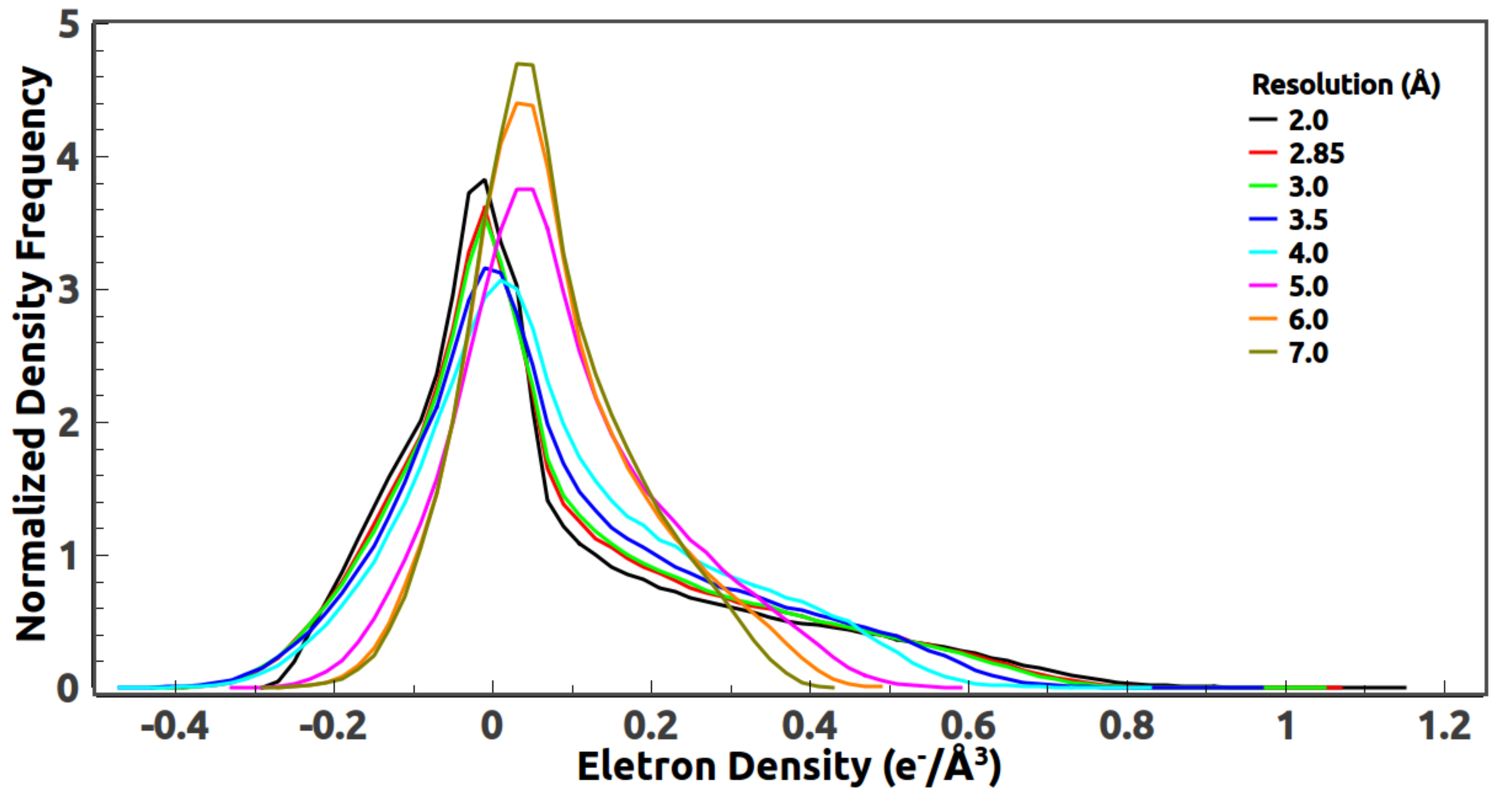
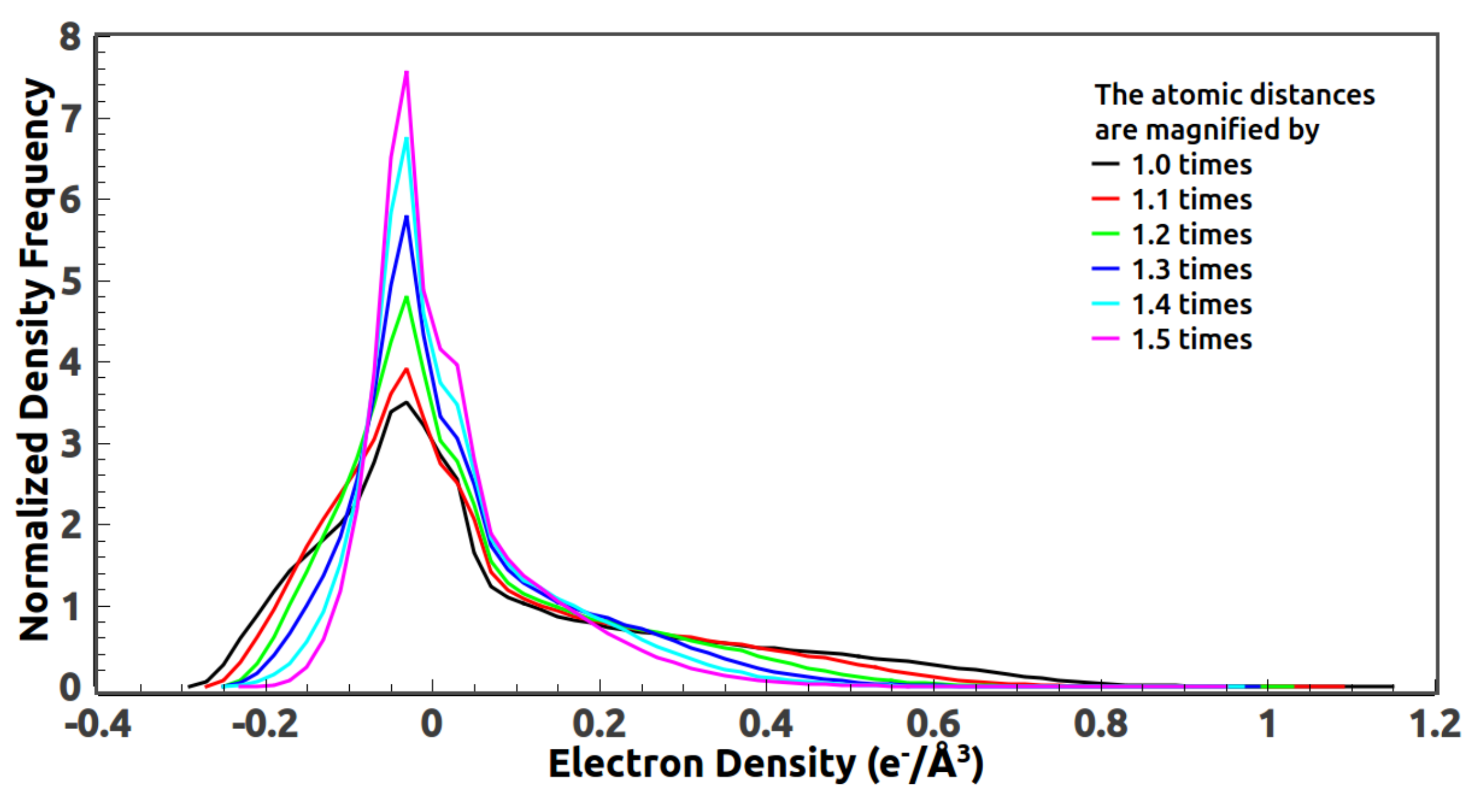
It is well-known that the density histogram is universal, i.e., independent of detailed structures. A question naturally arises, namely, what exactly does the histogram encode? Is that the average density of the protein or something else? Although this question is not directly related to the resolution dependence, we find this to be an interesting question to look at.
2. Ab Initio Phasing at Various Resolutions
Ab initio phasing using the HIO method has been described in previous articles [
13,
14,
15,
27,
28]. In this paper, we made 200 independent runs for each trial calculation and each run has 10,000 iterations. Each iteration consists of density modification in real space and using measured amplitudes in forward Fourier transform to improve phase values in reciprocal space. Before presenting the results of our trial calculations, let us briefly review the HIO phasing algorithm.
At the beginning of each iteration, data weighting [
12,
15] is used to speed up the convergence of the iterations and to increase the success rate. We give the diffraction data a weight defined in Equation (
1) where
varies with the iteration number.
is the reciprocal of the resolution (wavelength) of that reflection. The weighted data defined in Equation (
2) are used in the phasing process and updated at the beginning of each iteration. In the first iteration,
starts from a value of around 1.0 Å. The weight of high-resolution reflections are close to zero and only low- and medium-resolution reflections are involved in the phasing process. Due to a lower number of reflections involved, it helps the calculated protein boundary evolve to the correct shape which speeds up the phasing process and increases the success rate. Then
decreases smoothly in the following iterations which allows equal number of higher-resolution reflections be incorporated into the phasing procedure at each iteration until all reflections are involved at the 8000th iteration. Finally,
drops smoothly to zero from the 8000th to the 9000th iteration, so that observed reflections recover their original magnitudes. More details about how
varies have been described in our previous article [
15].
Missing reflections need to be filled with the calculated ones in each iteration. The beam stop used in the diffraction experiment often results in unmeasured reflections at very low resolution. The magnitudes of the missing reflections are replaced by the calculated values according to Equation (
3). This replacement is required in order to obtain a good electron density map in real space. About 1% of the observed data were randomly chosen and set aside as a test data set,
T, while the remainder were used as a work data set,
W [
29]. The reflections in the test data set should also be treated as missing reflections and replaced by the calculated values according to Equation (
3).
The electron density in a unit cell is defined on a grid. The grid size is chosen to be half of the high resolution limit of the phasing data. For example, the grid size is 1.43 Å for phasing 2.85 Å data, and 3.5 Å for phasing 7 Å data. Apparently, a bigger grid size leads to less computing time. However, a proper grid size is necessary in order to make sure all reflections to a given resolution have been involved in the computation.
INTEL forward and backward discrete fast Fourier transform [
30] is used to compute the electron density on each grid point in real space and the structure factors in reciprocal space.
The first iteration starts from random electron density in real space. A backward fast Fourier transform is performed to get the calculated structure factors in reciprocal space. The calculated magnitude of each reflection is replaced by the weighted observed magnitude defined in Equation (
2). The missing reflections are substituted with the calculated ones according to Equation (
3). The new magnitudes and the calculated phases are assembled to form new structure factors. A forward fast Fourier transform is performed to get the calculated electron density
in real space. The superscript
n denotes the
nth iteration.
In order to locate the protein boundary, a weighted average density on each grid point is calculated. Positive density constraint is applied during the calculation of the weighted average density, i.e., negative density is replaced by zero in the averaging. The density weighting function is defined in Equation (
4) [
7].
The subscript
i or
j represents a grid point in the asymmetric unit.
is the distance between the two grid points. The parameter
measures the width of a Gaussian function which can be used to control the convergence of the solvent region.
is chosen to be 4.0 Å at the first iteration and it decreases linearly in the following iterations. At the 9000th iteration,
is reduced to 2.5 Å, and it keeps that value when solvent flattening is applied during the last 1000 iterations. In practice, the weighted average density is calculated in reciprocal space according to the convolution theorem. More information about the calculation of the weighted average density can be found in our previous articles [
13,
14].
A cutoff value of the weighted average density is used to divide the asymmetric unit into the protein region and solvent region. The cutoff value can be found by adjusting it such that the calculated solvent content agrees with the expected solvent fraction. Since the average density of the protein is greater than the average density of the solvent, if a grid point has a weighted average density greater than the cutoff value, it is assumed to be inside the protein region. Otherwise, it is assumed to be part of the solvent.
After the protein boundary is determined, different density-modification techniques are employed to modify the calculated density in the solvent region and in the protein region, separately. In the solvent region, hybrid input-output introduces a negative feedback density according to Equation (
5) [
1,
2].
denotes the modified density of the nth iteration. is the density of the nth iteration before modification. is a feedback parameter which can be used to optimize the convergence of the algorithm. Empirically, is chosen to be 0.7. HIO does not change the calculated density of the protein region. Instead, a standard histogram-matching method is applied to make the calculated density in the protein region satisfy the density distribution of a reference histogram. After the density modification in real space, a backward fast Fourier transform is performed to get the calculated structure factors for the next iteration.
Since the HIO-modified density does not satisfy the solvent constraint, solvent flattening [
31,
32,
33,
34] is applied in real space during the last 1000 iterations according to Equation (
6).
Having reviewed the HIO phasing algorithm, we now proceed to describe the results of our trial calculations carried out for a membrane protein structure (PDB code 2JLN [
35]). 2JLN is a nucleobase-cation-symport-1 benzylhydantoin transporter which is an essential component of salvage pathways for nucleobases and related metabolites. The space group is P
. The cell dimensions are
,
, and
Å. The sequence includes 501 amino acids. Only 464 amino acids have been identified in the refined model. There are 3571 non-hydrogen atoms in the asymmetric unit. The crystal diffracts to 2.85 Å, with a low resolution cutoff at 29 Å. The completeness of the measured data is 88%. The overall R value after model refinement is about 0.24.
A proper value of solvent content is important for HIO phasing. The solvent content listed in PDB is 69% for 2JLN. After checking the model with
sfcheck [
36] in
CCP4 [
37], the volume not occupied by model is 68%. In our trial calculations, we have tested several values for the solvent content from 62% to 72%. Although all of them lead to successfully phasing, 68% turns out to be an optimal value with a high success rate and a low phase error.
For histogram matching, a protein structure (PDB code 4W6V [
38] of similar size is selected for the computation of a reference density histogram. 4W6V is a peptide transporter which mediates the cellular uptake of di- and tripeptides, and of peptidomimetic drugs. There are about 500 amino acids in the structure. Reference histograms from other structures of similar size also work. Since the histogram of a protein structure depends highly on the average temperature factor of the atomic model, the average B-factor of the reference structure should be rescaled to match the Wilson B-factor computed directly from the measured data of 2JLN. The reference histogram is computed at 2 Å resolution.
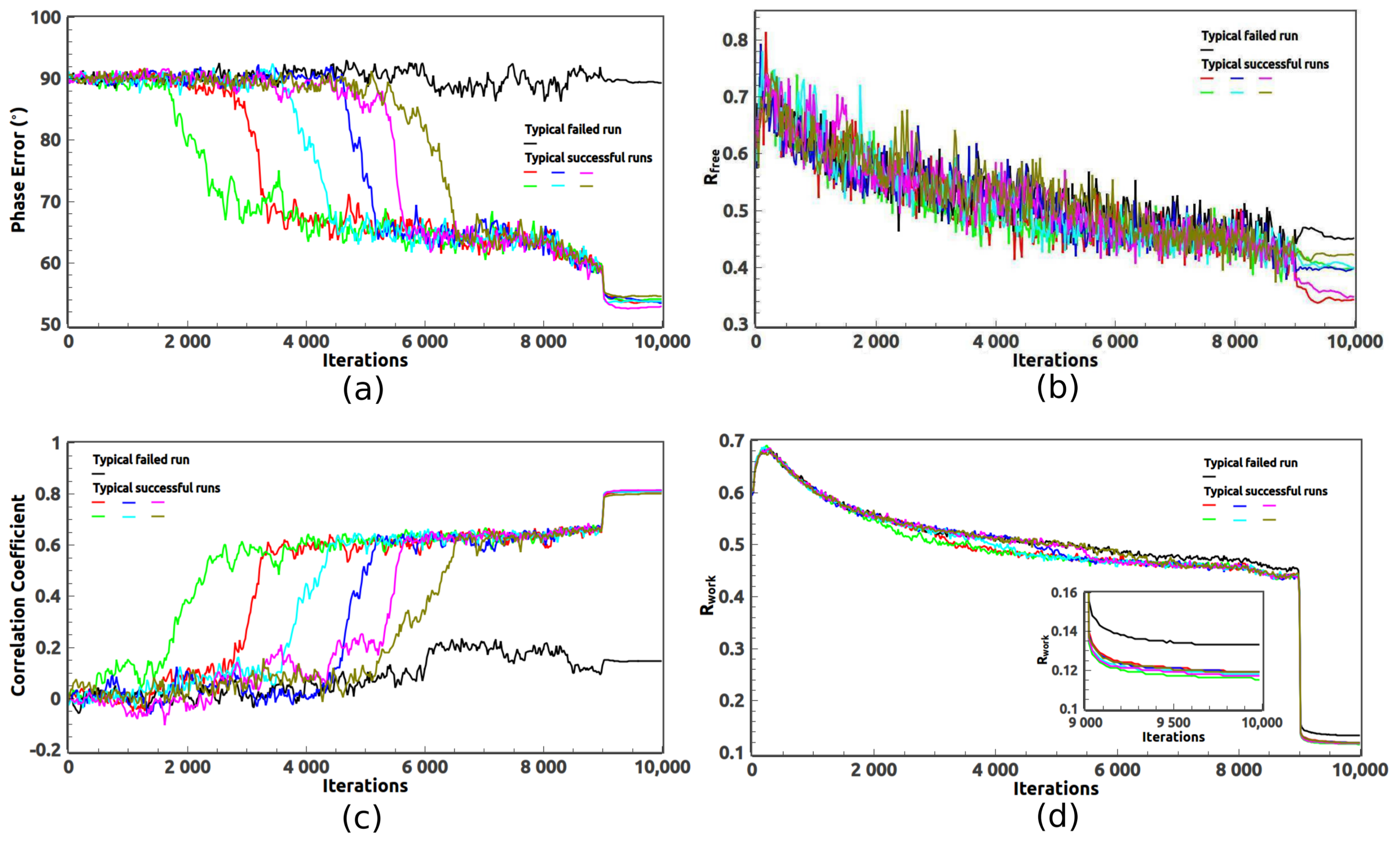
Several quantities are defined in Equations (7)–(10) to monitor the progress of the iterative phasing procedure. and measure the discrepancy between the calculated magnitudes and the observed magnitudes of the reflections in the test data set and the work data set, respectively. Since the phases of an unknown structure are not available, and should be used to identify whether good phases have been achieved. is a measure of the difference between the calculated phases and the true phases which are computed from the PDB deposited model with bulk solvent correction. The correlation coefficient, , is a measure of both calculated magnitudes and phases. The value of is close to one when good phases are achieved. Otherwise, it stays around zero.
Figure 1 shows the evolution of the error metrics defined in Equations (7)–(10). One typical failed run and six typical successful runs are presented. Initially, the phases are random and
is about 90
.
is close to zero. In a failed run, the phase error almost does not change significantly. The value of CC is close to zero. However, in a successful run, the phase error develops a sudden drop when good phases are achieved. The value of CC exhibits a sudden increase. For all runs, when the iterations proceed both
and
slowly decrease due to the progressively uniform data weighting. When solvent flattening is applied in the last 1000 iterations, the phase error further drops by several degrees and the CC value further increases.
also decreases but it can not discriminate between the failed and the successful runs due to the intermediate resolution of the measured data. However,
reached an obviously smaller value for those successful runs as shown in
Figure 1d and
Figure 2a. Therefore,
is still a good indicator when the resolution of the measured data is intermediate.
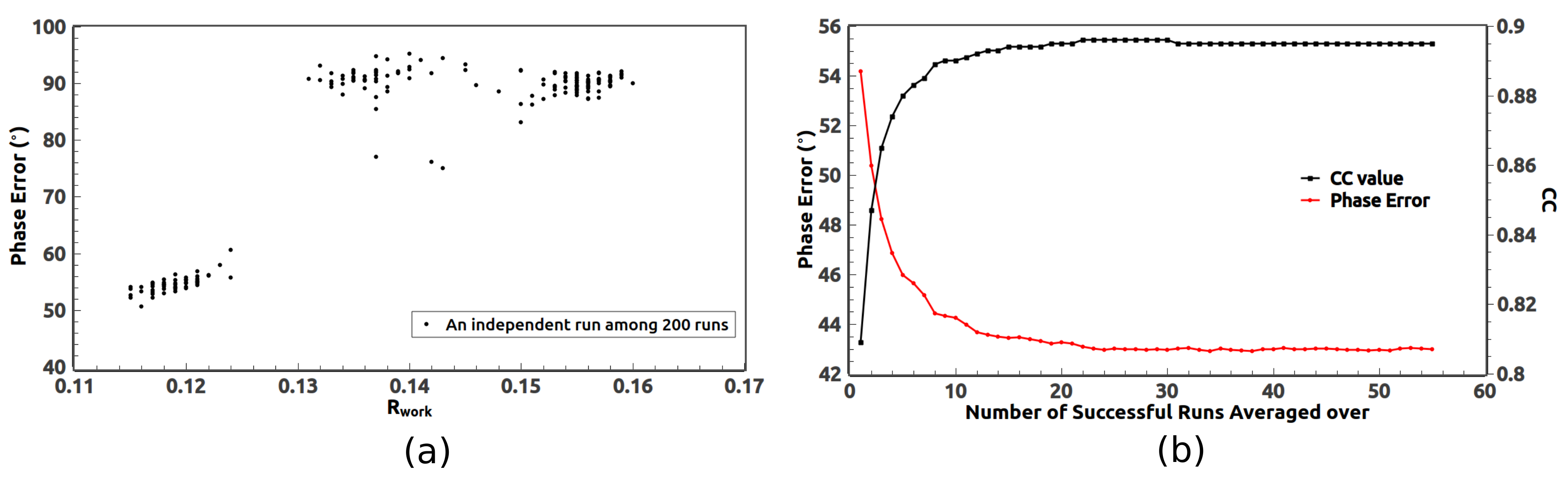
In order to identify those successful runs, we sorted
of the 200 runs in ascending order. We checked those runs with low
(less than 0.125 in
Figure 2a) and found that all of those runs are successful runs with small phase errors. We also found the lower the value of
, generally the smaller the phase error. On the other hand, those runs with high
correspond to failed runs with phase errors around
. There is a clear gap on the distribution of
in
Figure 2a which separates the failed group from the successful group.
of the failed group are not exactly the same. Some failed runs still contain some correct information about the protein boundary.
The successful runs form a set of low
(
Figure 2a) and they all correspond to a mean phase error around
. Since they started from different random phases, they approached the true phases from various directions. In other words, they are not identical due to statistical fluctuations. It is well known that averaging can reduce the fluctuations. As indicated in
Figure 2b, the mean phase error can be significantly reduced by averaging over those successful runs starting from the one with the lowest
and proceeding in the ascending order of
. Meanwhile, the CC value apparently increases. Therefore, averaging over those successful runs is a powerful phase improvement tool for the iterative phasing method.
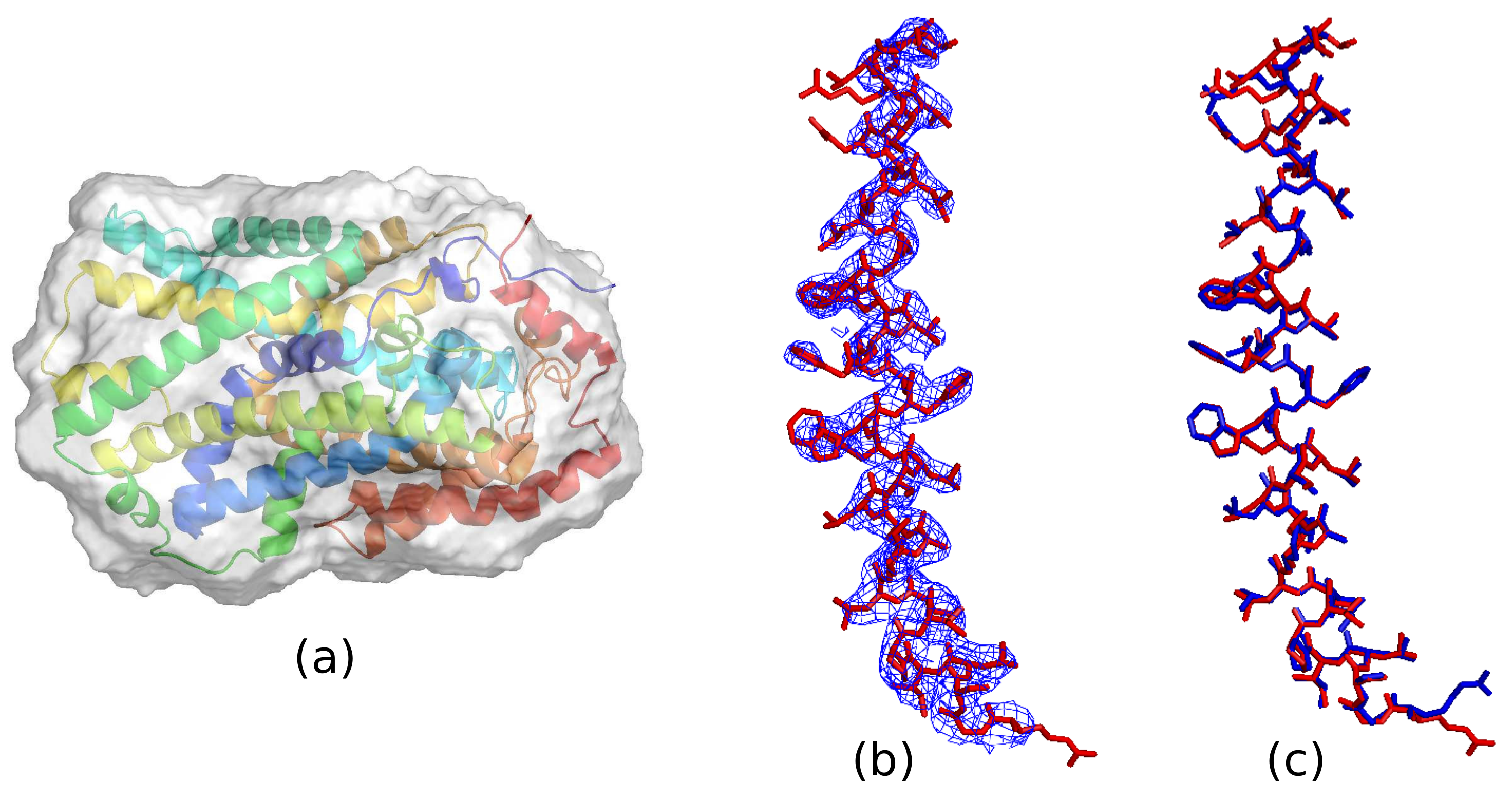
The calculated protein boundary of a typical successful run is shown in
Figure 3a. Evolving to a good boundary is crucial for the HIO method. If the protein density was not protected by a good boundary, HIO would destroy the calculated protein density during density modification and good phases would not be reached. A good comparison of the averaged density with the PDB deposited model is shown in
Figure 3b. Only one major helix of 2JLN is shown for clarity. The atomic model is well traced on the contour map of the averaged density. A model reconstructed from the averaged density using
ARP/wARP [
39] and
AutoBuild [
40] in
PHENIX [
41] is shown in
Figure 3c. The reconstructed model is quite close to the deposited model. About 81% of the 501 amino acids are positioned in the model. Further refinement is possible.
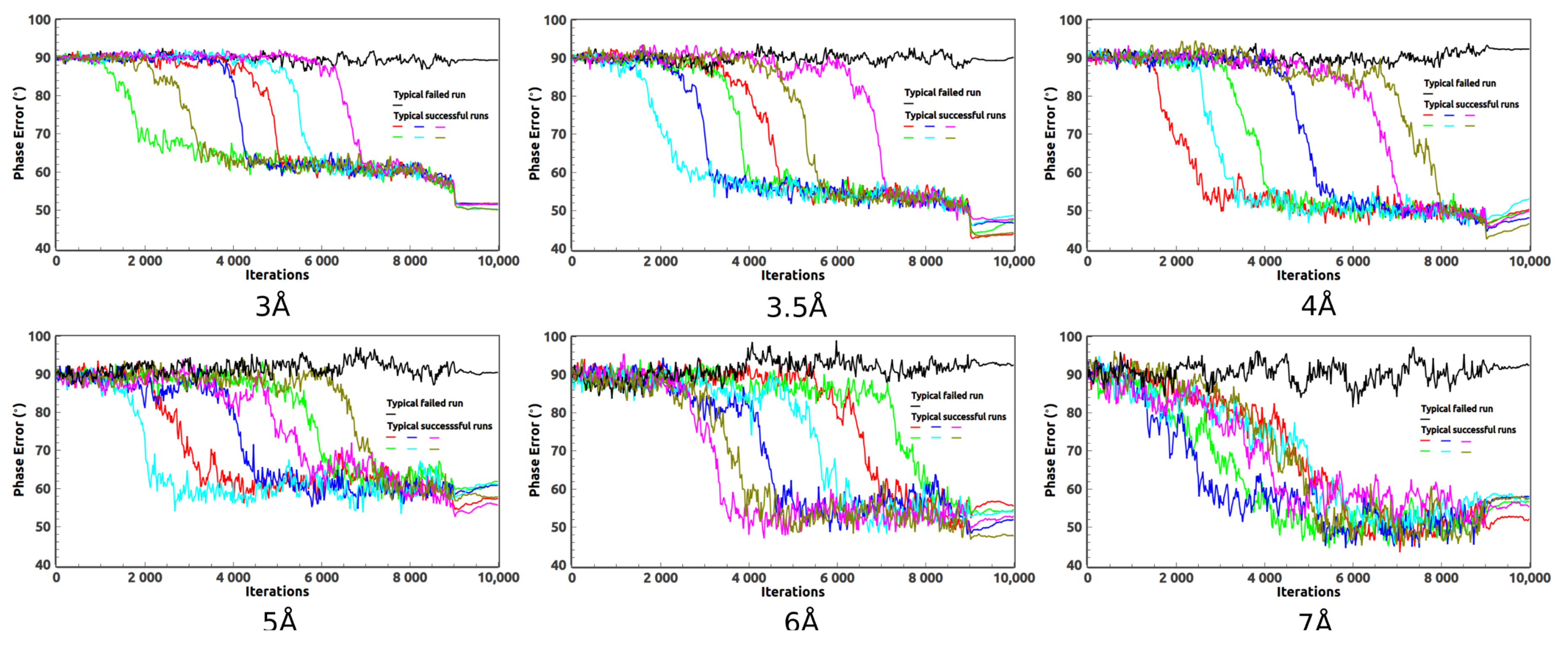
As the high-resolution data are not always available,
ab initio phasing of the medium- and low-resolution data is quite useful. In addition to the 2.85 Å data, we have also tried HIO phasing on the 3, 3.5, 4, 5, 6, and 7 Å data. For example, when phasing the 3 Å data, we pretend the measured data are limited to 3 Å. The evolution of the phase errors are displayed in
Figure 4. When phasing low-resolution data such as the 7 Å data, the expected density in the solvent region deviates a lot from a constant which weakens the power of the HIO method. As a result, a very low success rate is expected. A sudden drop of the phase error is no longer expected for those successful runs. If the resolution of the data goes much lower, such as 8 Å, it becomes difficult for the HIO method to achieve good phases for 2JLN.
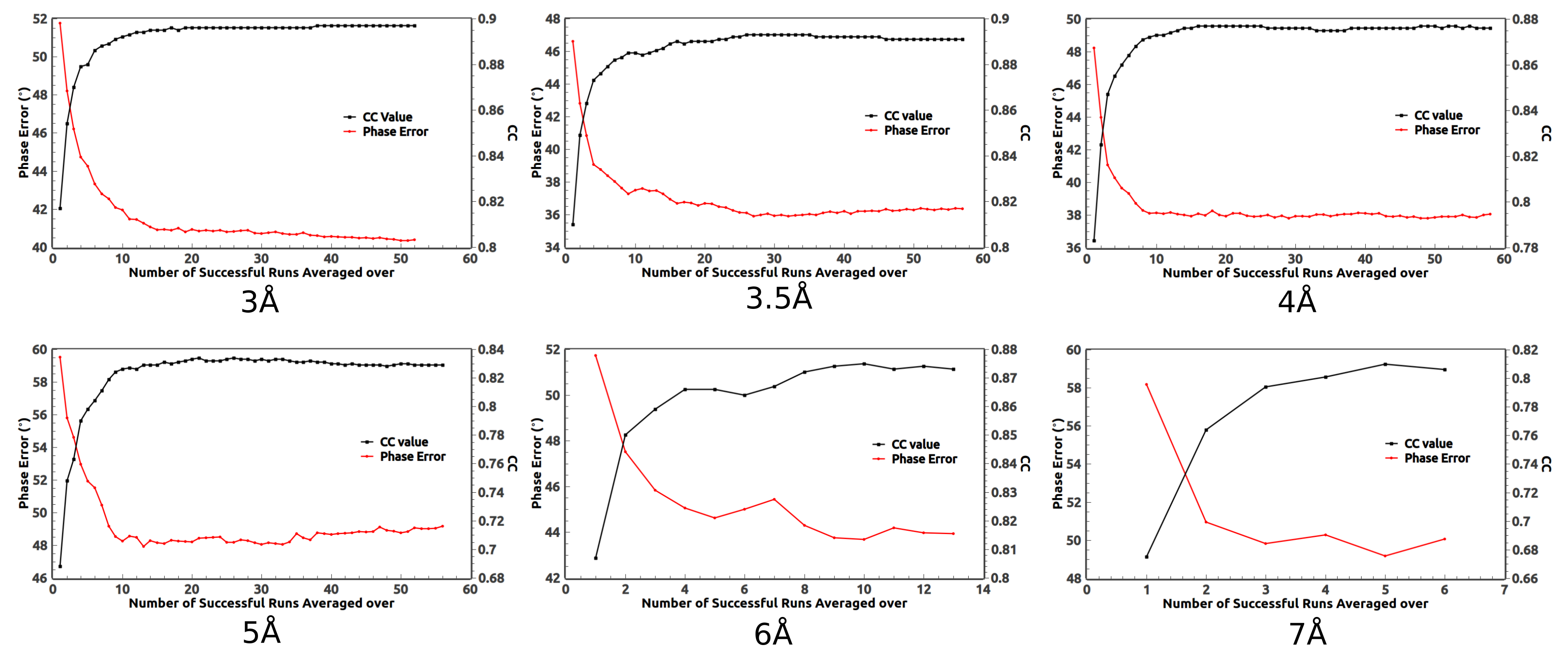
Like the 2.85 Å data, phase averaging over those successful runs can significantly improve the calculated phases of the medium- and low-resolution data as shown in
Figure 5. For the 3, 3.5, 4, and 5 Å data, there are around 50 successful runs among 200. After averaging over about 10 successful runs, the phase error becomes flat. It implies that less than 200 runs are needed in order to get the best phases. For the 6 and 7 Å data, since the success rate is low, more than 200 runs should be carried out. In fact, when averaging over more successful runs, better phases are obtained for the 6 and 7 Å data. On the other hand, averaging over too many runs may not be beneficial. In
Figure 5, the phase error of the 5 Å data slightly increases after averaging over too many runs.
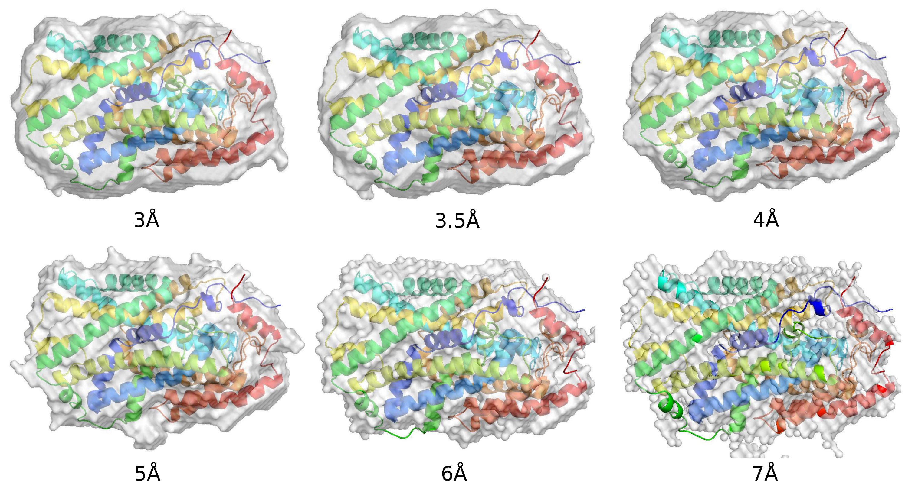
The calculated protein boundaries of typical successful runs for data of various resolutions are displayed in
Figure 6. For the 3, 3.5, 4, and 5 Å data, the reconstructed boundaries are smooth and well match the protein region. For the 6 and 7 Å data, small parts of some side chains get located outside of the calculated boundaries. The surfaces of the boundaries are rough due to the large grid size.
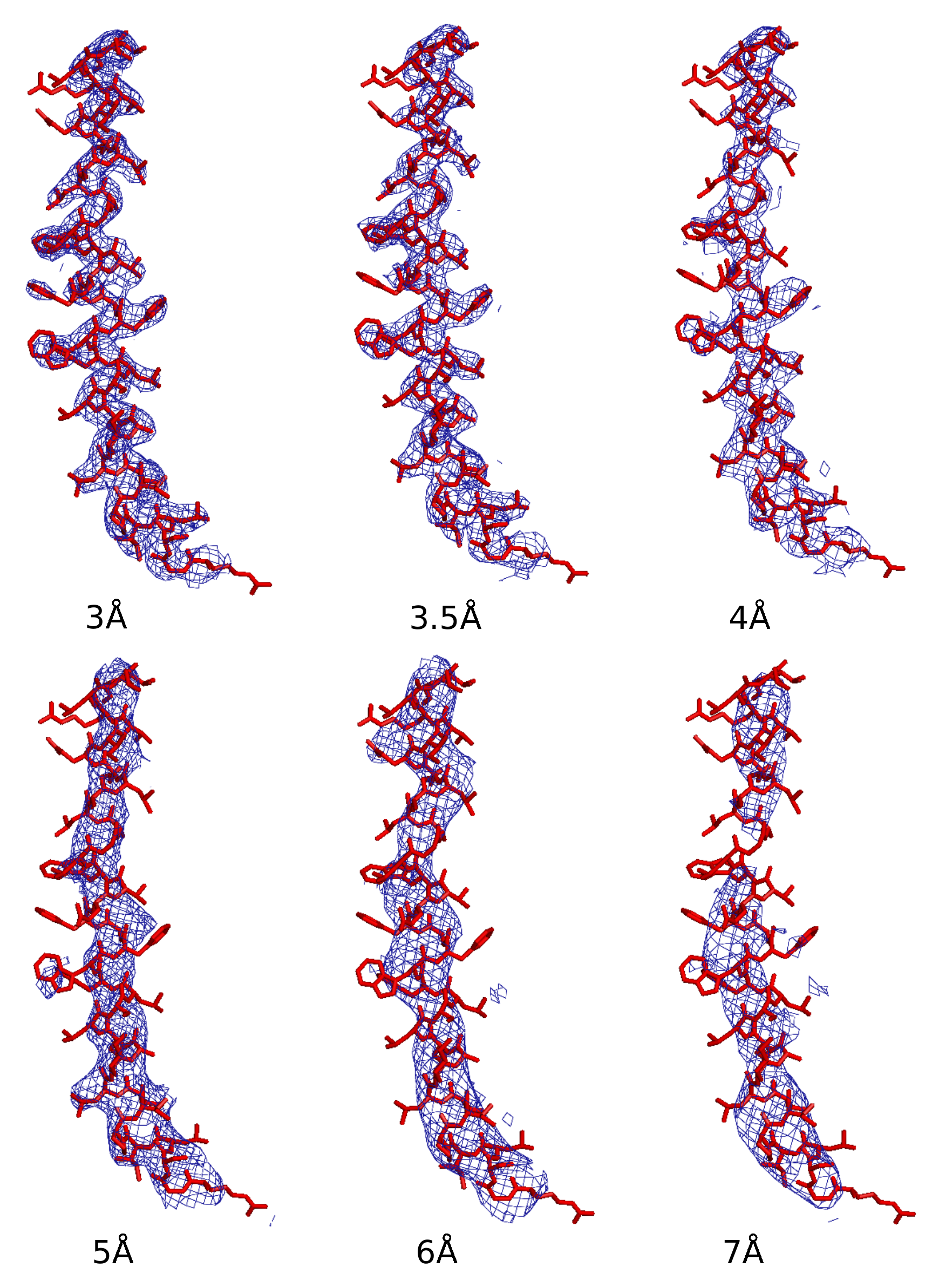
The averaged densities of those successful runs for data of various resolutions are shown in
Figure 7. The PDB deposited model is superimposed as a reference. Side chains can be traced on the density maps of the 3 and 3.5 Å data. For the 4 Å data, side chains are not very interpretable but the secondary structures are clearly visible. For the 5 and 6 Å data, secondary structures can be traced. For the 7 Å data, only partial secondary structures can be traced.
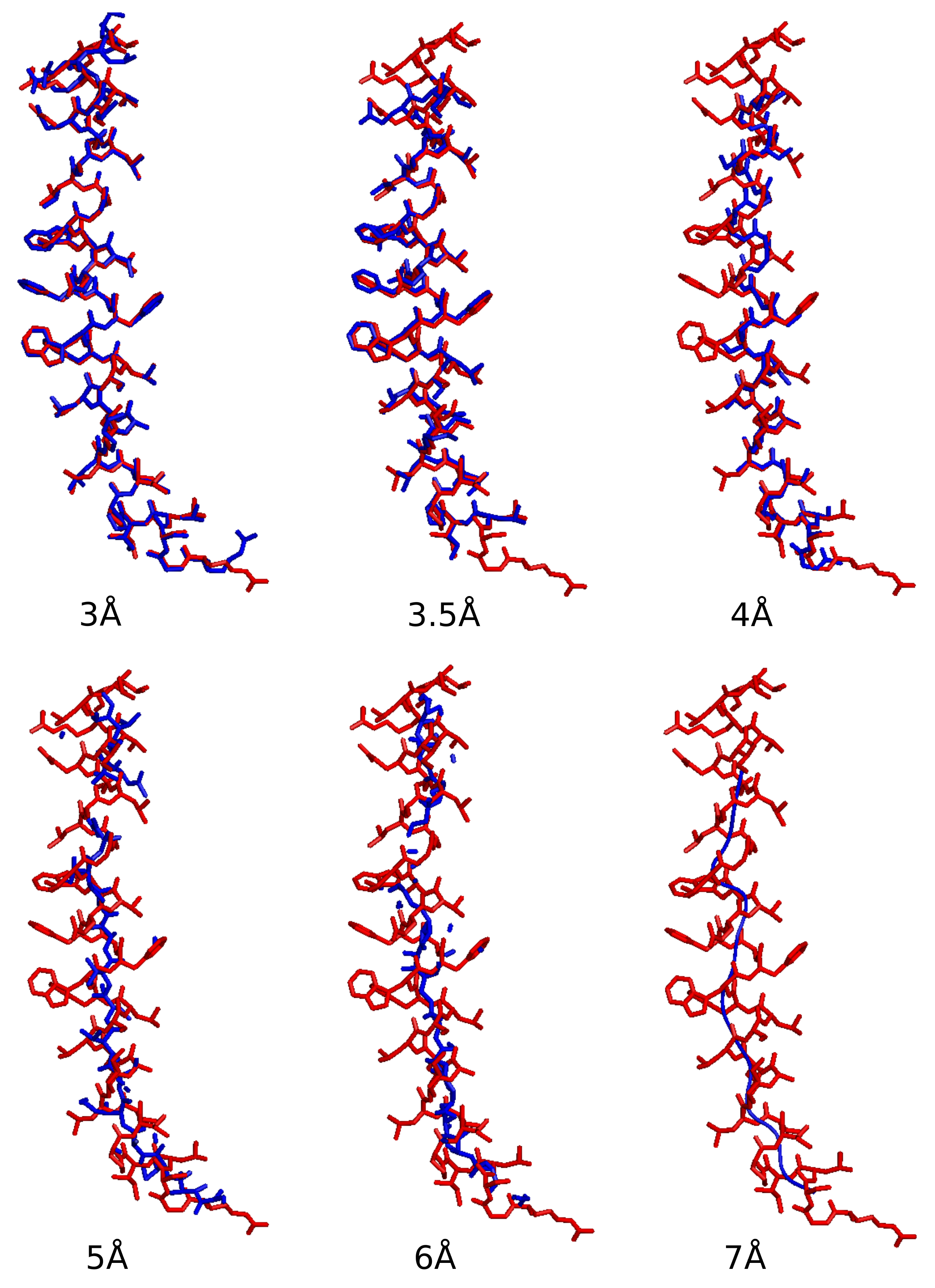
The reconstructed models of the averaged densities for data of various resolutions are displayed in
Figure 8. Side chains can be rebuilt for the 3 and 3.5 Å data using
ARP/wARP [
39]. Secondary structures can be clearly traced for the 4 Å data. They can be located for the 5 and 6 Å data, but not completely. For the 7 Å data, only partial helix can be traced.
In summary,
Table 1 lists the success rate, the final phase error, the final CC value, and the completeness of the reconstructed models for data of various resolutions. For the 2.85, 3, 3.5, 4, and 5 Å data, the number of successful runs are around 55 among 200. For the 6 and 7 Å data, the success rates decrease a lot. Overall, the final phase errors are less than
and the final CC values are above 0.8. The completeness of the reconstructed model declines when the resolution of the data decreases, as the expected density in the solvent region is not flat for low-resolution data, which is not favorable to the HIO method. For the 8 Å data, no successful runs have been reached. The 3 Å data seems better than the 2.85 Å data in rebuilding the model. That is probably because the measured data in the resolution shell from 2.85 to 3 Å contain more errors which can be seen in
Figure 9a.


