Abstract
In cholesteric liquid crystals (CLC) problems related to the localized optical modes for a non-collinear geometry are studied here in the two wave dynamic diffraction theory approximation. This approximation, which insures the results accuracy order of δ (where δ is the CLC dielectric anisotropy), is applied because for a non-collinear geometry there is no exact analytic solution of the Maxwell equations and a theoretical description of the experimental data becomes more complicated. The dispersion equation for non-collinear localized edge modes (called conical modes (CEM)) is found and analytically solved for the case of thick layers and for this case the lasing threshold and the conditions of the anomalously strong absorption effect are found. It is shown that qualitatively CEMs are very similar to the localized edge modes (EM) in CLCs related to a collinear geometry, i.e., for the case of light propagation along the spiral axis however the CEMs differ by their polarization properties (the CEM eigen polarizations are elliptical ones depending on the degree of CEM deviation from the collinear geometry in contrast to the circular eigen polarizations in the EM case). What is concerned of the CEM quantitative values of the parameters they are “worth” (the photonic effects are not so pronounced) than for the corresponding ones for EM. The CEM lasing threshold is higher than the one for EM, etc. Performed theoretical studies of possible conversion of EMs into CEMs showed that it can be due to the EM reflection at dielectric boundaries at the conditions of a high pumping wave focusing. Known experimental results on the CEM are discussed and optimal conditions for CEM observations are formulated.
1. Introduction
Recently there are very intense experimental and theoretical activities in the field of localized optical modes (edge modes (EM) and defect modes (DM)) in chiral liquid crystals (CLC) mainly due to the possibilities to reach a low lasing threshold for the distributed feedback (DFB) lasing [1,2,3,4], to use the defect modes as narrow band filters [5,6] and to enhance the nonlinear optical high harmonic generation [7] in chiral liquid crystals. The localized EM and DM exist as a localized electromagnetic eigenstate in a CLC layer or at a structure defect in the layer with its frequency outside of the forbidden band gap (for EMs) or in the forbidden band gap (for DMs). EM and DM were investigated initially in the three-dimensionally periodic dielectric structures [5]. The corresponding EMs and DMs in chiral liquid crystals, and more general in spiral media, are very similar to the corresponding modes in one-dimensional scalar periodic structures. They reveal abnormal reflection and transmission outside (for EMs) and inside (for DMs) the forbidden band gap [1,2] and allow DFB lasing at a low lasing threshold [3]. A qualitative difference with the case of scalar periodic media is connected with the polarization properties. It should be noted that most studies of the localized EM and DM are related to the localized modes in collinear geometry, i.e., for the case of light propagation along the spiral axis [1,2,3]. Much less attention was paid to the localized modes in CLC for noncollinear geometry. It is due to the fact that all photonic effects in CLC are most pronounced just for the collinear geometry and also partially due to the fact that a simple exact analytic solution of the Maxwell equations is known for the collinear geometry, whereas for a noncollinear geometry there is no exact analytic solution of the Maxwell equations and a theoretical description of the experimental data becomes more complicated. It is why in papers related to the localized modes in CLC for a non-collinear geometry and observing phenomena similar to the case of collinear geometry [8,9,10,11,12,13] their interpretation is not so clear. Meanwhile, theoretical approaches based on numerical calculations and approximate theory were widely applied to the conventional CLC optics in non-collinear geometry and are used insufficiently for the non-collinear (conic) localized modes in CLC, in particular, for the non-collinear (conical) edge localized modes (CEM). The term “conic” used for the non-collinear geometry appeared because in an experiment a set of CEMs, emitted in a cone formed around the CLC axis, are usually observed simultaneously. In spite the fact that an individual CEM is formed by a superposition of only two plane waves propagating at an angle to the CLC axis, the cone arises because the CEM energy is degenerated on the propagation directions of the mentioned plane waves (their wave vectors directions) if these directions are formed by both wave vectors simultaneous rotation around the CLC axis.
The present paper is aimed for a partial covering of the mention gap in the theoretical description of the collinear and non-collinear localized modes presenting below an approximate analytic theory of CEM in CLC in the framework of two-wave dynamical diffraction theory and its application to the non-collinear DFB lasing in CLC. Recently, a paper [14] devoted to the conical edge modes of higher diffraction orders in photonic liquid crystals was published. This paper is devoted to an application of the presented in the present paper general two-wave dynamical diffraction theory to some specific simple case where essential simplifications occur. In particular, eigen polarizations are the linear ones and for a second diffraction order as a small theory parameter appears the squared CLC dielectric anisotropy δ2.
2. CLC Eigen Waves at Oblique Incidence
To describe conical localized edge modes in CLC (CEM), as it was done in [15] for the case of collinear geometry, one has to know eigen waves in CLC in the process of solving a boundary problem. An exact finding of eigen waves in CLC for non-collinear geometry demands a numerical approach to the problem. However, there is a small parameter for CLC, namely, the local dielectric anisotropy δ, which allows us to apply an approximate approach, the two-wave dynamical diffraction theory. It means that close to the Bragg condition an electromagnetic wave in CLC being a sum of many Bloch harmonics is approximated by a sum of the two most pronounced harmonics. The problem of eigen waves in CLC for non-collinear geometry (as well the optical problems of a CLC layer: reflection, transmission, etc.) in the two-wave dynamical diffraction approximation was solved by Belyakov and Dmitrienko with coworkers (see [16,17]). It was found that in this approximation the eigen wave in a CLC might be presented as a superposition of two elliptically polarized plane waves with the ellipticity of polarization depending on the angle between the helical axis and the wave propagation direction. So, in the solving of a boundary problem (see Figure 1) determining CEM we shall use the known eigen waves expressions [16,17]:
where q± are the additions to the wave vectors due to diffraction, σ+ and σ− are the unit vectors of elliptical polarizations, and the wave vectors K± are related by the Bragg condition via τ, the CLC reciprocal lattice vector (τ = 4π p, where p is the CLC pitch), δ = (ε1 − ε2)/(ε1 + ε2) is the CLC dielectric anisotropy (with ε1 and ε2 being the principal values of CLC dielectric tensor), ε0 = (ε1 + ε2)/2, κ = ωε0½/c the z-axis is directed along the spiral axis, and kt is the wave vector tangential component. In (1) j labels four eigen waves [16,17].
E(r,t) = e−iωt [E+σ + exp(iK+z)+ E− σ−exp(iK− z)]exp(iktr), K+ − K− = τ, Kj+ = τ/2 ± q±,
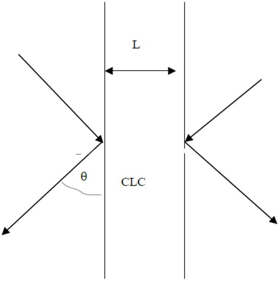
Figure 1.
Schematic of the boundary problem for conical edge modes.
The polarizations vectors σ+ and σ− may be presented in the form:
where ex and ey are orthogonal unit vectors perpendicular to the wave vectors of plane waves forming the eigen waves, and αi and βi are parameters determining the type of polarizations. For example, αi = π/4 and βi = π/2 (−π/2) correspond to the right and left circular polarizations, respectively.
σi = (cosαiex + eiβ sinαiey),
In the two-wave dynamical diffraction approximation the dependences on the propagation direction and the frequency of the polarization vectors σ+ and σ− and other parameters in (1) have to be found from the solution of the equation
which after substitution in it (1) reduces to the following system of two vector linear equations [16,17]:
where ε0, ετ, and ε−τ are the only nonzero Fourier expansion components of the CLC dielectric tensor [16,17]. A detailed analysis of the eigen waves in CLC, in particular, their polarization properties, at an oblique light propagation was performed in [16,17]. It was found that in a typical situation two eigen waves with “diffracting” elliptical polarizations (and with the corresponding q− in (1)) experience diffraction scattering and two others with “non-diffracting” (or weakly diffracting with the corresponding q+ in (1)) elliptical polarizations are very weakly influenced by the diffraction scattering. For a normal incidence, as it is well known, these polarizations are reduced to the left and right circular polarizations. For a non-collinear geometry the eigen waves polarization vectors are slightly changing inside the stop-band (at variations of the wavelength or the propagation direction).
RotRot E = c−2ε(z)∂2 E/∂t2,
(ε0 − K+2/κ2) E+ σ+ + ετ E− σ− = 0, ε−τ E+ σ+ + (ε0 − K−2/κ2)E−σ− = 0,
As an approximation for the eigen waves polarization vectors (neglecting their changes inside the stop-band) a kinematic expression may be taken into account for the eigen polarizations (see Equations. (2.19) and (2.21) in [17]). If we assumed that the vector ex in (2) lies in the scattering plane formed by the wave vector K+ and K− the parameter β in (2) becomes equal to π/2 and the kinematic approximation gives:
α = ±arctgsinθ.
Since localized modes, in particular CEM, are connected with diffracting eigen-waves in CLC we shall restrict the consideration below only to the diffracting eigen-waves.
For diffracting eigen-waves the general expressions describing eigen-waves [16,17] may be simplified. Nevertheless, the polarization vectors have to be found from the general expressions [16,17]. In the case of a CLC layer with its surfaces being perpendicular to the helical axis (see Figure 1) the Bragg condition relates to the parallel to τ tangential components of the wave vectors entering in (1) and tangential components of the wave vectors for the diffracting eigen-waves are determined by the formula
where α = τ(τ + 2k)/k2 is the parameter determining deviation of the wave vector from the Bragg condition and 2θ is the angle between the wave vectors of two plane waves in eigen wave (1), or the scattering angle. The ratio of amplitudes (E−/E+) in the two diffracting eigen waves determined by the Equation (1) is given by the expression
Kjt+ = τ/2 ± q,
q = (τ/4)[(α)2 − (δ/2)2(1 + sinθ)2]½,
ξ+ = (E−/E+)± = (δ/2)(1 + sinθ)/{α ± [(α)2 − (δ/2)2 (1 + sinθ)2].
Note, that the general expression for parameter α = τ(τ + 2k)/k2 reduces to α = 2(Δω/ωB)sinθB for a changing the frequency by Δω at the fixed incidence angle and to α = 2ΔθsinθB for a changing the incidence angle by Δθ at the fixed frequency, where ωB and θB are the Bragg frequency and the Bragg angle, respectively.
3. Boundary Problem in Noncollinear Geometry
One can begin consideration of the boundary problem in the formulation, which assumes that a plane optical wave of diffracting polarization is obliquely incident at the planar CLC layer. The amplitudes of the two eigen waves E±+ and E±− excited in the layer by the incident wave (with the amplitude of incident wave equal to unity and a propagation direction close to the one determined by a wave vector in the CLC eigen wave) are determined by the following equations
where L is the layer thickness.
E++ + E−+ = 1,
exp[i Kt−+L]ξ+ E++ + exp[iKt−−L]ξ−E−+ = 0,
The amplitude reflection Ra and transmission Ta coefficients for light of diffracting polarization take the form:
Ra = −i(δ/2)(1 + sinθ)(sinqL)/[(4q/τ)cosqL − iαsinqL].
Ta = (4q/τ)exp[iτL/2]/[(4q/τ)cosqL − iαsinqL].
The reflection R = |Ra|2 and transmission T = |Ta|2 coefficients experience oscillations versus the frequency outside the stop-band. In nonabsorbing layers the relation R + T = 1 holds for all frequencies. At q = nπ/L, where n is an integer number, R = 0 and T = 1.
As it is known [15] the dispersion equation for an edge mode can be obtained as a condition of solvability of a homogeneous equation obtained from Equation (6), i.e., zero value of the Equation (6) determinant:
tg(qL) = −4i(q/τ)/α.
In a general case the solution of Equation (10) determining the CEM frequencies (ωCEM) can be found only numerically. The CEM frequencies ωCEM occur to be complex quantities, which may be presented as ωCEM = ω0CEM(1 + iΔ), where Δ (determining imaginary part of frequency) in real situations is a small parameter. So, the localized modes are weakly decaying in time, i.e., they are quasistationary modes. Luckily, an analytic solution may be found for some limiting case, namely, for a sufficiently small Δ ensuring the condition (qL)Im(q/τ) << 1. In this case the values of a real part of ωCEM, i.e., ω0CEM, are coinciding with the frequencies of zero values of the reflection coefficient R for a nonabsorbing layer and the complex CEM frequencies are determined by the relations:
where n is an integer number numerating CEMs.
(Lq) = nπ, Δ = −(1/4)δ(1 + sinθ))(nπ)2/[(δ/2) (1 + sinθ) Lτ/4]3,
The CEM life-time in this limiting case is
where c is the speed of light.
τCEM = (Lε0½/c)[L(δ/2)(1 + sinθ)/pn]2,
In the found solution of the homogeneous system (8) the eigen solutions amplitude ratio is −1 and the electromagnetic field inside the layer is a superposition of two eigen waves of the form determined by Equation (1) with the found from the homogeneous system the amplitude ratio E−+/ E++ = −1.
The following from (1) expression for the electromagnetic field inside the layer is given by the formula
where ωn is the nth CEM frequency, qn and ξn± are determined by the dispersion Equations (10) and (7), respectively, and r┴ is the radius-vector parallel to the layer surface. In the limiting case of (qL)Im(q/τ) << 1 the qn is determined by the expression (11) and the expression (12) reduces to a more simple formula:
where the exact value qn is substituted by an approximate value qn = nπ/L. The presented (13,14) eigen solution of the boundary problem is localized in a layer of thickness L standing wave with being modulated along the z amplitude. The number of modulation periods at the layer thickness L is coinciding with the CEM number n. The CEM energy density distributions along the layer normal following from Equation (12) for the CEM numbers n = 1, 2, and 3 are shown in Figure 2. The Figure 2 presents a total energy density distribution in the layer along the normal to its surfaces.
E(z, r┴,t) = exp[i(r┴kcosθ − ωnt)][2σ+iexp(iτz/2)sin(qnz) + σ−exp(−iτz/2)(ξn+exp(iqnz) −
ξn−exp(−iqnz))],
ξn−exp(−iqnz))],
E (z, r┴,t) = exp[i(r┴kcosθ − ωnt)][2σ+iexp(iτz/2)sin(nπz/L) + σ−exp(−iτz/2)(ξn+exp(i nπz/L) −
ξn−exp(−i nπz/L))],
ξn−exp(−i nπz/L))],
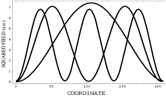
Figure 2.
Calculated non-collinear localized edge modes (CEM) energy density (arbitrary units) versus the coordinate (in the dimensionless units zτ) inside the layer for the three first CEMs (δ(1 + sinθ)/2 = 0.05, N = 33, n = 1, 2, and 3).
However, in each point of the layer the total density is presented by two plane waves propagating in the different directions, so one may calculate separately for any point in the layer the intensities of waves propagating in the different directions. Figure 3 shows the energy density coordinate distributions of the waves propagating inside and outside of the layer close to the layer surfaces.
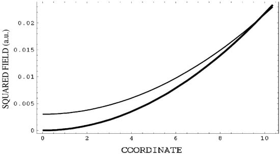
Figure 3.
Calculated CEM energy (arbitrary units) distributions close to the chiral liquid crystal (CLC) layer surface versus coordinate (in the dimensionless units zτ) for a plane wave directed inside (bold line) and outside the layer for the first edge mode (δ(1 + sinθ)/2 = 0.05, N = 16.5, n = 1).
One can see that at the layer surface the energy density of the wave propagating inside the layer was strictly zero, however, for the same point the energy density of the wave propagating outside the layer was not zero, however small. It means that the CEM energy was leaking from the layer through its surfaces. The expression for the leaking wave amplitude at the layer surface follows from Equation (12) and for [δ(1 + sinθ)Lτ/8] >> 1 looks as
|E|out = (2τnπ/(δ(1 + sinθ)L))/τ2 = 2nπ/(τLδ(1 + sinθ)).
For sufficiently thick layers and for growing layer thickness L the CEM life-time τm grows as a third power of the thickness and is inversely proportional to the square of the CEM number n2 (see (12)).
A similarity of the solutions for EM and CEM should be commented here. Since for both collinear (exact solution) and non-collinear (approximate solution for conical modes) cases the eigen-waves were presented as a superposition of two plane-waves the resulting equations were similar. However, the expressions for specific parameters entering in these similar equations were different.
4. Absorbing CLC
Let us examine now CEM in an absorbing CLC. The motivation of this study, in particular, was due to the anomalously strong absorption effect known in the photonic properties [18,19]. The formulas of the preceding sections were examined in more detail assuming for simplicity that the absorption in the layer is isotropic. The absorption of an optical medium was described here by using a wave vector with nonzero imaginary part. We defined the ratio of the wave vector imaginary part to its real part as γ, i.e., k = k0 × (1 + iγ), where k0 is the real part of wave vector. Note, that in the actual situations γ << 1. At Figure 4 1-R-T (total absorption) calculated versus the real part of the wave vector are presented for several values of positive γ.
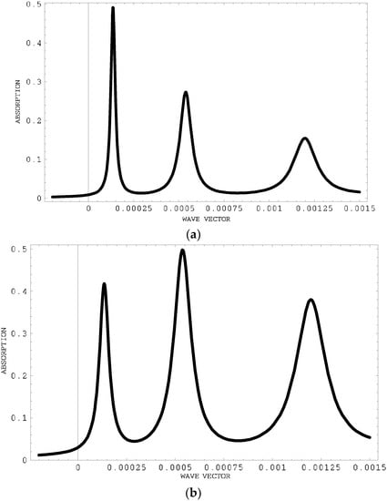
Figure 4.
Total absorption in the layer (1-R-T) calculated versus the dimensionless wave vector kd = δ(1 + sinθ)/2[2(2ksinθ − τ)/τ(δ(1 + sinθ)/2 − 1)] (i.e., normalized by the Bragg wave vector the difference of the wave vector and the Bragg wave vector); N = 700, δ(1 + sinθ)/2 = 0.03) (a) for γ = 0.0002 and (b) γ = 0.0007.
At Figure 4 and at all figures below the frequency (wave-vector) dependencies of different CEM characteristics at a fixed light propagation direction are presented. Very similar angular dependencies at a fixed frequency were revealed in the calculations because the parameters determining these dependencies on variations of the frequency and the propagation angle (see the explanations to (7)) were identical.
The absorption reveals energy beats close to the edge of the selective reflection band with the maxima positions coinciding with the locations of R minima. The most simple situation corresponds to the case of a >> 1 where a = δ(1 + sinθ) Lτ/8 = δ(1 + sinθ)πL/2p.
For small γ and (τL)Im(2q/τ} << 1 the following from Equation (9) the intensity reflection, transmission coefficients and total absorption at the frequencies of reflection minima (11) are reduced to the following expressions:
R = 4[a3 γ/δ(1 + sinθ)]2/[(nπ)2 + 2a3 γ/δ(1 + sinθ)] 2
T = (nπ)4/[[(nπ)2 + 2a3 γ/δ(1+ sinθ)]2.
1 − (R + T) = [4(nπ)2a3γ/δ(1 + sinθ)]/[(nπ)2 + 2a3 γ/δ(1 + sinθ)]2
It follows from (16) that for each n maximal absorption, i.e., maximal 1-R-T, occurs for (nπ)2 = 2a3 γ/δ(1 + sinθ). It means that the maximal absorption occurs for a special relationship between n, γ, the propagation direction and L and if this relationship, i.e., (nπ)2 = 2a3γ/δ(1 + sinθ), is fulfilled R = 1/4, T = 1/4, and 1 − R − T = 1/2.
Due to the assumed smallness of γ, this result corresponds to a strong enhancement of the absorption for weakly absorbing layers. The absorption enhancement may be observed by direct measuring of 1-R-T. However, from the experimental point of view, as a more easy way of measuring of the intensity of some inelastic process, for example, measuring of the secondary produced fluorescence [20]. The anomalous strong absorption may be used for the CEM detection, however the most efficient detection demands special interconnection of the problem parameters. Really, as Equation (16) shows the absorption maximum corresponds to (nπ)2 = 2a3γ/δ(1 + sinθ). Since γ is determined by the layer substance, so for the maximum absorption a special relation between the propagation direction, period, layer thickness, and amplitude of effective dielectric constant modulation has to be fulfilled to ensure equality
γ = (δ/2[δ(1 + sinθ)πL/2p]3)(1 + sinθ)(nπ)2 = (2πn)2 /[δ2 (1 + sinθ)2 (πL/p)3].
If the Equation (17) is applied to a pumping wave it shows that the absorption maximum can be achieved by a changing of the pumping wave propagation direction. The effect was experimentally observed in [20,21].
5. Amplifying LC
We now assumed that γ < 0, which means that the CLC is amplifying. If |γ| is sufficiently small, the waves emerging from the layer according to Equation (8) exist only in the presence of at least one external wave incident on the layer, and their amplitudes are determined by the solution of Equation (8), i.e., by Equation (9). In this case (see Figure 5c) R + T > 1 or 1-R-T < 0, which just corresponds to the definition of an amplifying medium.
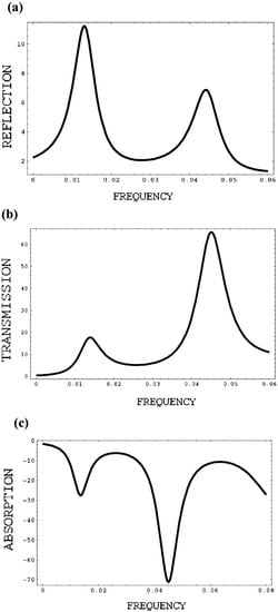
Figure 5.
R (a), T (b), total absorption 1-R-T (c) calculated here and at all figures below versus the dimensionless frequency ωd = δ(1 + sinθ)/2[2(ωsinθ − ωB)/ωBδ(1 + sinθ)/2 − 1)], where ωB = cτ/2ε02 (i.e., normalized by the Bragg frequency the difference of the frequency and the Bragg frequency); (l = 300, l = Lτ, δ(1 + sinθ)/2 = 0.05) for γ = −0.009, i.e., for the gain between the thresholds for the first and the second edge modes.
However, if the imaginary part of the dielectric tensor, i.e., γ, reaches some critical negative value, the quantity R + T diverges and the amplitudes of waves emerging from the layer are nonzero even for zero amplitudes of the incident waves. This happens when the determinant of Equation (8) reaches zero value. At this point, of course, the amplitudes of emerging waves are not determined by the solution (9) of linear equations (a nonlinear problem should then be solved). However, as we saw above, the points of reducing the determinant of Equation (8) to zero determine the CEM and the corresponding values of the gain (or the negative imaginary part of the dielectric tensor), i.e., the minimum threshold gain at which the conic lasing occurs (see the corresponding discussion for EM in spiral and scalar periodic media in Ref. [22,23,24,25]).
Therefore, the equation determining the threshold gain (γ) at which the lasing occurs (zero value of the determinant of Equation (8) or of the denominator in (9)) turns out to coincide with Equation (10). However, it should be solved now not for the frequency but for the imaginary part of the dielectric constant (γ). In the general case, this equation has to be solved numerically. However, for a very small negative imaginary part of the dielectric tensor, the CEM frequency values are pinned to the frequencies of zeros of the reflection coefficient in its frequency beats outside the stop-band edge for the same layer with a zero imaginary part of the dielectric tensor [23,26,27]. This is why the threshold values of the gain for the CEM can be represented by analytic expressions in this limit case.
To the lasing at the CEM frequencies corresponds the threshold values of γ (i.e., a minimum |γ| at which the lasing occurs for n-th reflection minimum):
γ = −4(nπ)2/ [δ2(1 + sinθ)2(Lτ/4)3].
As can be seen from (18), the threshold values of |γ| are inversely proportional to the third power of the layer thickness, increases with the angle θ decrease, and the minimum value of |γ| corresponds to n = 1, i.e., to the EM closest to the selective reflection band edge (cf. analogous results for EM in a scalar layered media [24,25]). The values of γ given by the Equation (18) are convenient to use for estimating the threshold values of γ in the general case and as a zero approximation in the numerical solution of Equation (10) for the threshold values.
It also follows from Figure 6 that the different threshold values of γ (at divergent R and T) correspond to the different CEM numbers n in Figure 6a–d. This means that individual lasing modes can be excited by changing the gain (γ). If the value of γ is between the consequent threshold values of γ for neighboring CEM, the lasing may not be achieved and the layer may reveal only amplifying properties (see Figure 5a–c). This means that changing the pumping wave intensity allows achieving lasing at the individual CEM and that the lasing intensity is not a monotonic function of the pumping intensity. Since the lasing frequency is determined by the CEM frequencies, there is an option for some variation of the lasing frequency and the CEM number inside the width of the dye line by changing the CLC pitch or by variation of the angle θ.
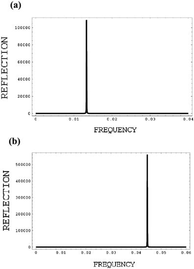
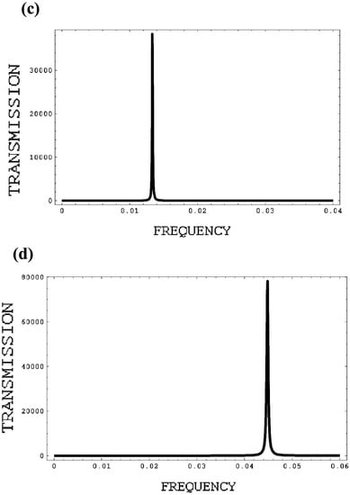
Figure 6.
Calculated frequency dependence of R (l = 300, l = Lτ, δ(1 + sinθ)/2 = 0.05) (a) close to the threshold gain for the first lasing edge mode (γ = −0.00565), (b) close to the threshold gain for the second lasing edge mode (γ = −0.0129); calculated frequency dependence of T (l = 300, l = Lτ, δ(1 + sinθ)/2 = 0.05), (c) close to the threshold gain for the first lasing edge mode (γ = −0.00565), and (d) close to the threshold gain for the second edge mode (γ = −0.0129).
The obtained above results show that qualitatively the CEM properties are very similar to the EM (localized mode in a collinear geometry) ones. The revealed for EMs important effects (anomalously strong absorption, low DFB lasing threshold, etc.) exist also for CEMs. However, there are some essential differences related first of all to the CEM eigen mode polarizations and to more weak than for EM realization of the mentioned above effects. In particular, the DFB lasing threshold is higher for CEM in comparison with EM. It is a direct consequence of the fact that in the equations determining the lasing threshold for CEM instead δ, entering for EM, enters a smaller quantity δ(1 + sinθ)/2. So, consequently, the more the propagation direction deviation from the normal to the layer is the higher lasing threshold for CEM is. This explains an easier obtaining of EM (collinear) lasing compared to the CEM lasing in the experiment.
6. Possible Coupling between Localized Modes
The considered above eigen solutions of the boundary problem describing CEM were obtained for a perfect CLC layers without of jumps of the averaged dielectric constant at the layer surfaces and in the assumption that the layer size is infinite. Since the Maxwell equations giving CEM solutions are linear the found in our approximation (assuming infinite layer size and neglecting by the dielectric reflection at the layer surfaces) CEM and EM solutions have no options of a transfer between themselves. However, in a real experiment with an averaged dielectric constant jump at the layer surfaces, a finite layer size and possible CLC sample imperfections, coupling between eigen solutions of the boundary problem describing localized modes are not forbidden by the conservations laws in the framework of linear theory. Moreover, the experiment [10,12,13] gives examples of such coupling between optical localized modes.
It is why we shall study below a possible coupling between optical localized modes (in particular, between EM and CEM) in the framework of a phenomenological linear theory. An excitation of CEM by an EM may be caused by the EM field Fresnel reflection at the layer surfaces with non-coinciding averaged dielectric constants of the CLC layer and the external medium. As it is well known at a dielectric (Fresnel) reflection of a circularly polarized light the chirality sense of the circular polarization is changing (light of a left polarization transforms to the reflected light of right polarization and vice versa). So, a reflected at one layer surface EM produces in CLC a plane wave of a non-diffracting polarization propagating along the CLC axis. After reflection at the opposite CLC layer surface this plane-wave transforms again in a plane wave of a diffracting polarization. This process results in a renormalization of EM due to the surface scattering [27]. However, other transformation processes are also possible.
We shall consider below the excitation of a CEM via an EM. Excitation of CEM in a non-amplifying CLC layer requires an incident at the CLC layer external wave (waves) of the frequency coinciding with the CEM frequency. This role may be played by a double reflected at the layer surfaces one of the EM plane waves composing EM in a collinear geometry. In this case the CEM amplitude is determined by the equation, which differs from Equation (4) only by an addition to the right hand side of the system (4) some terms originating due to the mentioned above EM reflections at the boundaries. The general solution of the system found from (4) by adding to it inhomogeneous terms may be presented as a superposition of the particular solution corresponding to the inhomogeneous system obtained from (4) by adding in its right hand side of the double reflected wave and the solution corresponding to the homogeneous system (4), i.e., corresponding to the CEM. The coefficients in this superposition have to be determined from the boundary conditions.
The inhomogeneity Ei to be added to the system (4) is of the form
where R(L) and R(0) are the amplitude reflection coefficients with changing of the circular polarization chirality sense in reflection at the dielectric jumps for the both layer surfaces, nd is the polarization vector of diffracting circular polarization, and kn is the wave vector of light with non-diffracting polarization at a propagation direction along the CLC axis.
Ei ~ exp(iK+z)R(L)R(0)exp(iknL)nd,
One can easily construct the solution of the inhomogeneous Equation (4) as a sum of general and particular solutions. For this, it is sufficient to present amplitudes E++ and E−+ in the form
where E++C, E−+C and E++p, and E−+p are the amplitudes of eigen waves in the CEM and in the particular solution, respectively. To obtain an explicit form of the equations for E++C, E−+C and E++p, and E−+p one has to project the inhomogeneity (19) at the CEM polarization vector σ+ and perform its Fourier transform.
E++ = E++p + E++C, E−+ = E−+p + E−+C,
Taking into account that the amplitudes E±+C satisfy Equation (4) (with zero right hand sides) one obtains
for the frequencies close to the CEM frequencies ωCEM. The expression for CEM amplitudes (21) is proportional to the projection of the inhomogeneity (19) Fourier transform at the CEM polarization vector σ+. For an infinite CLC layer the inhomogeneity Fourier transform is proportional to the delta-function δ(k-KEM+), where KEM+ is the wave vector entering in the EM solution, i.e., KEM+ is directed along the CLC axis. Since the wave vectors entering in the CEM solution (see (1)) have a perpendicular to the CLC axis addition, i.e., they differ from KEM+, the inhomogeneity added to the right side of Equation (4) for an ideally perfect unlimited CLC layer is effectively reduced to zero and CEM can not be excited by EM in an ideally perfect unlimited CLC layer. Nevertheless, in a real CLC layer due to its limited size or imperfections a possibility of CEM being excited by EM remains because the uncertainty relation between the wave vector and coordinate ΔkΔr ≈ 1. So, a layer size limitation by Δr (i.e., limitation of the beam cross-section) results in the uncertainty of the perpendicular to the CLC axis wave vector component order of 1/Δr, which allows a CEM excitation by EM if it does not contradict to the conservation laws. It also should be mentioned that a limited CLC layer surface might be taken into consideration due to a finite area of the EM excitation by a pumping wave (usually a laser beam is focused at a small spot at the layer surface). So, we could reveal a qualitative dependence on some parameters of the problem of the inhomogeneity finally entering in Equation (4):
where εe is the external medium dielectric constant.
E±+C = ±E++[1 + itg(qL)],
σ*+Ei ~ σ*+nd(ε0½ − εe½)2,
If in CLC there is a CEM of the same frequency as the one of the EM the studied above process of a double surface scattering results also in the CEM excitation.
Since the CEM frequency in CLC is higher than the EM frequency the only option for a CEM excitation by the EM is an EM at the high frequency stop-band edge inducing a CEM at the low frequency stop-band edge. If one is talking about a coupling between EM and CEM in a regime of lasing it should be assumed that the source of excitation is lasing at EM frequency because the EM lasing threshold is lower than the one for CEM. A similar connection between two CEMs, one at the high frequency stop-band edge and other at the low frequency stop-band edge, is also possible with the angle θ for the low frequency edge exceeding the corresponding angle for the high frequency edge.
The presented above mechanism of CEM exciting via EM due to the scattering at interfaces with a dielectric constant jump can be applied for an alternative explanation of the observed in [12] exciting of CEM at EM lasing (case IV in the notations of the authors of [12] explained in [12] by an “anomalous scattering”). The proposed in the present paper mechanism predicts quite definite dependences of the CEM exciting on the experimental parameters (jump of dielectric constant, angle of deviation from collinear geometry, and size of the focused pumping beam spot), which can be directly verified in the experiment. Qualitatively these dependences look as the following: the amplitude of excited CEM is proportional to the squared difference of refractive indexes of CLC and external medium (due to reflection), decreasing with increasing the deviation from collinear geometry (angle θ decreasing), growing with decreasing the focused pumping beam spot (resulting in increasing of the inhomogeneity (19) Fourier transform), and, naturally, proportional to the EM amplitude.
For the CEM excitation by this mechanism there is no need in lasing at the EM frequency. The CEM can be excited via an EM excitation in the framework of a linear optical process without the lasing (the corresponding observation was reported in [12]). An investigation of the stop-band structure for an oblique incidence using fluorescence in the framework of the linear optics was reported in [28]. The EM and CEM coupling was also recently investigated in [29], where, in particular, was found that a focusing of the pumping wave promotes the coupling realization (which is in a full agreement with the above discussion).
7. Conclusions
The performed above analytic description of CEM was an approximate (based at the two-wave dynamical diffraction theory), however, for many cases it might be regarded as an exact from the practical point of view, because the results accuracy was determined by a small parameter, the dielectric anisotropy δ. If the experiment demanded higher accuracy the solution obtained in the framework of the presented approach might be regarded as a zero approximation in subsequent numerical calculations. What is concerned of the qualitative results, without doubts, they were correctly described in the present approach. The said relates to the conclusion that the lasing threshold for the CEM is higher than for EM (collinear lasing geometry), to the CEM polarization properties, etc. The obtained analytical results can be easily applied to the CEM in scalar photonic media.
Some general property of CEM should be also mentioned. This localized at the layer thickness (in one dimension) modes are propagating along the layer surface electromagnetic structures with a propagation speed depending on the structure deviation from the collinear geometry (angle θ). So, if the EM is a motionless electromagnetic structure, the CEM is moving along the layer surface electromagnetic structure with the phase velocity equal to ccosθ. So, this property can be a base for the CEMs apparent using in time-delay lines for light.
As a most direct use of the presented analytical results on CEM may be regarded by their application to many experimental observations of conical edge modes (see [8,9,10,11,12] and references in [12]) for clarification of the observed phenomena physics and formulating optimal conditions for observation and application of the corresponding effects.
The work is supported by the State Assignment “0033-2019-0001”.
Funding
This research was funded by the Russian Academy of Sciences under the State Assignment “0033-2019-0001”.
Acknowledgments
The work is supported by the State Assignment “0033-2019-0001”.
Conflicts of Interest
The authors declare no conflict of interest.
References
- Yang, Y.-C.; Kee, C.-S.; Kim, J.-E.; Park, H.Y.; Lee, J.C.; Jeon, Y.J. Photonic defect modes of cholesteric liquid crystals. Phys. Rev. E 1999, 60, 6852. [Google Scholar] [CrossRef] [PubMed]
- Kopp, V.I.; Genack, A.Z. Double-helix chiral fibers. Phys. Rev. Lett. 2003, 89, 033901. [Google Scholar] [CrossRef] [PubMed]
- Schmidtke, J.; Stille, W.; Finkelmann, H. Defect mode emission of a dye doped cholesteric polymer network. Phys. Rev. Lett. 2003, 90, 083902. [Google Scholar] [CrossRef] [PubMed]
- Shibaev, P.V.; Kopp, V.I.; Genack, A.Z. Photonic materials based on mixtures of cholesteric liquid crystals with polymers. J. Phys. Chem. B 2003, 107, 6961. [Google Scholar] [CrossRef]
- Yablonovitch, E.; Gmitter, T.J.; Meade, R.D.; Rappe, A.M.; Brommer, K.D.; Joannopoulos, J.D. Donor and acceptor modes in photonic band structure. Phys. Rev. Lett. 1991, 67, 3380. [Google Scholar] [CrossRef] [PubMed]
- Hodgkinson, I.J.; Wu, Q.H.; Torn, K.E. Chiral liquid crystal as narrow band filters. Opt. Commun. 2003, 184, 57. [Google Scholar] [CrossRef]
- Hoshi, H.; Ishikava, K.; Takezoe, H. Enhanced nonlinear optical high harmonic generation in chiral liquid crystals. Phys. Rev. E 2003, 68, 020701R. [Google Scholar] [CrossRef]
- Lee, C.-R.; Lin, S.-H.; Yeh, H.-C.; Ji, T.D.; Lin, K.L.; Mo, T.S.; Kuo, C.T.; Lo, K.Y.; Chang, S.H.; Fuh, A.Y.; et al. Color cone lasing emission in a dye-doped cholesteric liquid crystal with a single pitch. Opt. Express 2009, 17, 1290. [Google Scholar] [CrossRef]
- Lee, C.R.; Lin, S.H.; Ku, H.S.; Liu, J.H.; Yang, P.C.; Huang, C.Y.; Yeh, H.C.; Ji, T.D.; Lin, C.H. Spatially band-tunable color-cone lasing emission in a dye-doped cholesteric liquid crystal with a photoisomerizable chiral dopant. Appl. Phys. Lett. 2010, 96, 111105. [Google Scholar] [CrossRef]
- Lin, S.-H.; Lee, C.-R. Novel dye-doped cholesteric liquid crystal cone lasers with various birefringences and associated tunabilities of lasing feature and performance. Opt. Express 2011, 19, 18199. [Google Scholar] [CrossRef][Green Version]
- Ying, C.-F.; Zhou, W.-Y.; Li, Y.; Ye, Q.; Yang, N.; Tian, J.-G. Multiple and colorful cone-shaped lasing induced by band-coupling in a 1D dual-periodic photonic crystal. AIP Adv. 2013, 3, 022125. [Google Scholar] [CrossRef]
- César, L.; Folcia, J.O.; Etxebarria, J. Cone-shaped emissions in cholesteric liquid crystal lasers: The role of anomalous scattering in photonic structures. ACS Photonics 2018, 5, 4545–4553. [Google Scholar]
- Folcia, C.L.; Ortega, J.; Etxebarria, J. Anomalous light scattering in photonic cholesteric liquid crystals. Liq. Cryst. 2019. [Google Scholar] [CrossRef]
- Belyakov, V.A.; Semenov, S.V. Localized conical edge modes of higher orders in photonic liquid crystals. Crystals 2019, 9, 542. [Google Scholar] [CrossRef]
- Belyakov, V.A.; Semenov, S.V. Optical edge modes in photonic liquid crystals. J. Exp. Theor. Phys. 2009, 109, 687–699. [Google Scholar] [CrossRef]
- Belyakov, V.A.; Dmitrienko, V.E. Optics of cholesteric liquid crystals. Sov. Phys. Solid State 1974, 15, 1811. [Google Scholar] [CrossRef]
- Belyakov, V.A. Diffraction Optics of Complex Structured Periodic Media (Localized Optical Modes of Spiral Media); Springer: Berlin, Germany, 2019; Chapter 3. [Google Scholar]
- Belyakov, V.A.; Gevorgian, A.A.; Eritsian, O.S.; Shipov, N.V. Anomalous absorption in cholesterics. Zh. Tekhn. Fiz./Sov. Phys. Tech. Phys. 1987, 57, 843–845. [Google Scholar]
- Belyakov, V.A.; Dmitrienko, V.E. Optics of chiral liquid crystals. In Soviet Scientific Reviews/Section A, Physics Reviews; Khalatnikov, I.M., Ed.; Harwood Academic Publisher: Reading, UK, 1989; Volume 13, pp. 1–203. [Google Scholar]
- Etxebarria, J.; Ortega, J.; Folcia, C.L. Anomalous fluorescence in chiral liquid crystal. Liq. Cryst. 2017, 45, 122. [Google Scholar] [CrossRef]
- Moreira, M.F.; Relaix, S.; Cao, W.; Tahery, B.; Palffy-Muhoray, P. Liquid crystals microlasers. In Transword Reaserch Network; Blinov, L., Bartolino, R., Eds.; Transworld Research Network: Karala, India, 2010; p. 223. [Google Scholar]
- Kopp, V.I.; Zhang, Z.-Q.; Genack, A.Z. Lasing in chiral photonic structures. Prog. Quantum Electron. 2003, 27, 369. [Google Scholar] [CrossRef]
- Kogelnik, H.; Shank, C.V. Coupled-wave theory of distributed feedback lasers. J. Appl. Phys. 1972, 43, 2327. [Google Scholar] [CrossRef]
- Yariv, A.; Nakamura, M. Periodic structures for integrated optics. J. Quantum Electron. 1977, 13, 233. [Google Scholar] [CrossRef]
- Shabanov, V.F.; Vetrov, S.Y.; Shabanov, A.V. Optics of Real Photonic Crystals; RAS, Sibirian Branch: Novosibirsk, Russia, 2005. (In Russian) [Google Scholar]
- Belyakov, V.A. Localized optical modes in optics of chiral liquid crystals. In New Developments in Liquid Crystals and Applications; Choudhury, P.K., Ed.; Nova Publishers: New York, NY, USA, 2013; Chapter 7; pp. 199–227. [Google Scholar]
- Belyakov, V.A.; Semenov, S.V. Localized optical modes in chiral liquid crystals with Local Absorption Anisotropy. JETP 2014, 118, 798–813. [Google Scholar] [CrossRef]
- Risse, A.M.; Schmidtke, J. Angular-dependent spontaneous emission in cholesteric liquid-crystal films. J. Phys. Chem. C 2019, 123, 2428–2440. [Google Scholar] [CrossRef]
- Nys, I.; Stebryte, M.; Ussembayer, Y.Y.; Beeckman, J.; Neyts, K. Mode coupling by scattering in chiral nematic liquid crystal ring lasing. Opt. Express 2019, 27, 8081–8091. [Google Scholar]


© 2019 by the author. Licensee MDPI, Basel, Switzerland. This article is an open access article distributed under the terms and conditions of the Creative Commons Attribution (CC BY) license (http://creativecommons.org/licenses/by/4.0/).