1. Introduction
To study the molecular mechanisms of complex diseases like cancer, microscopic images can provide valuable information, but it is often necessary to carry out a series of molecular biology experiments on several conditions [
1,
2]. Traditionally, the images from the experiments have been evaluated manually. Thus, it was time-consuming and needed a lot of human effort and expertise. Therefore, with the emerging development of high-content and high-throughput digital imaging systems, it is necessary to design new and automated analysis tools for current microscopic images. Among the variety of tasks done using microscopic images, cell counting is one of the crucial ones [
3]. The number of cells in a microscopic image can be used as a measurement to be compared among different groups. For example, we can evaluate the treatment effect of a cancer drug at different doses by comparing the microscope-based cancer cell counts under the specified conditions [
2]. Hence, the experimental group with the smallest cell count number in its microscopic images may be treated as the first dosage of the drug to be used for that specific cancer. The same principle can be applied to identify the most effective drugs as well [
4]. Therefore, it is important for biologists to automatically collect accurate cell counts for each of the experimental groups under different experimental conditions so that further statistical significance can be modeled and evaluated.
In computer vision field, automated counting objects in static images have been mostly studied and practiced for crowd counting in pedestrian traffic to decrease traffic crash fatalities [
5]. According to the review by Loy et al., there are two major strategies for automated object counting in static images: counting by detection and counting by regression [
6]. Counting by detection was the earliest method used in object counting. It involves first training an object detector, then applying the detector to the whole image using a sliding window or other segmenting technique to identify the objects and estimate the number of objects [
5,
7,
8]. Many detectors have been proposed and evaluated in different studies, but the performance of these detectors still has room for improvement, especially when the resolutions of the images are low and some of the objects in the images are overlapped [
5,
7]. Counting by regression is considered to be a more accurate and faster strategy [
6]. A typical counting by regression study first employs a preprocessing step to extract low-level features like size, area, histogram, and texture, and high-level features like object foreground segment map, dot density representative map, etc., and then regresses these features to the object counts [
8,
9]. The preprocessing step can be implemented manually or automatically. A lot of efforts have been made to extract robust features automatically. For example, artificial neuron network (ANN), a well-studied machine learning algorithm inspired by the human neuron network, can be involved in both the feature extraction step and the regression step, and has been confirmed to have good performance on both tasks [
10].
Among the features used in previous object counting studies, foreground masks and dot density maps have gained more and more attention in recent years due to the rapid development of deep artificial neural network (DANN) and autoencoder techniques [
11]. DANN is a kind of special ANN with more hidden nodes and layers in its architecture, and it is also known as deep learning (DL) [
12]. Autoencoder refers to a model strategy which usually consists of a contracting block to compress data from the input layer into a short code and a symmetric decoding block which enables that short code to be decompressed into something that closely matches the original data. For the two popular types of features mentioned above, a foreground mask is a kind of white and black binary image. Pixels in the objects (e.g., cancer cells) in the images are white (foreground), while pixels of the background are black [
13]. Dot density maps aim to specify object position by putting a single dot on each object instance in each image [
9]. These two types of features themselves can be plotted out as images and have the same sizes as their original images. Hence, using them as annotations or labels requires us to build powerful autoencoder-like architectures. Fortunately, the emerging DANN-based autoencoder technology provides us with more options.
By introducing a convolution operation into a DANN model, the DANN is turned into a deep convolutional neural network (DCNN). DCNN is widely used in computer vision due to its power in handling structured data like image data, and it has been applied to cell counting tasks. Xie et al. designed several fully connected DCNN models to first predict the dot density map, then sum the dots in the map up as the estimated count in a microscopic image [
14]. The advantage of the density-based method is that it has the potential to address cell overlapping. However, this method is sensitive to the variances of datasets. When applying the algorithm to a varietal dataset rather than the one similar to the training set, extra fine-tuning work is necessary. Hernández et al. built a DCNN-based autoencoder named feature pyramid network (FPN) to generate foreground feature masks of microscopic images, then applied another DCNN model to regress the mask to cell count [
10]. This strategy is more direct and does not need extra sum-up and fine-tuning steps for different datasets, but this kind of segmentation-based method cannot overcome limitations such as cell clumping and overlap [
7].
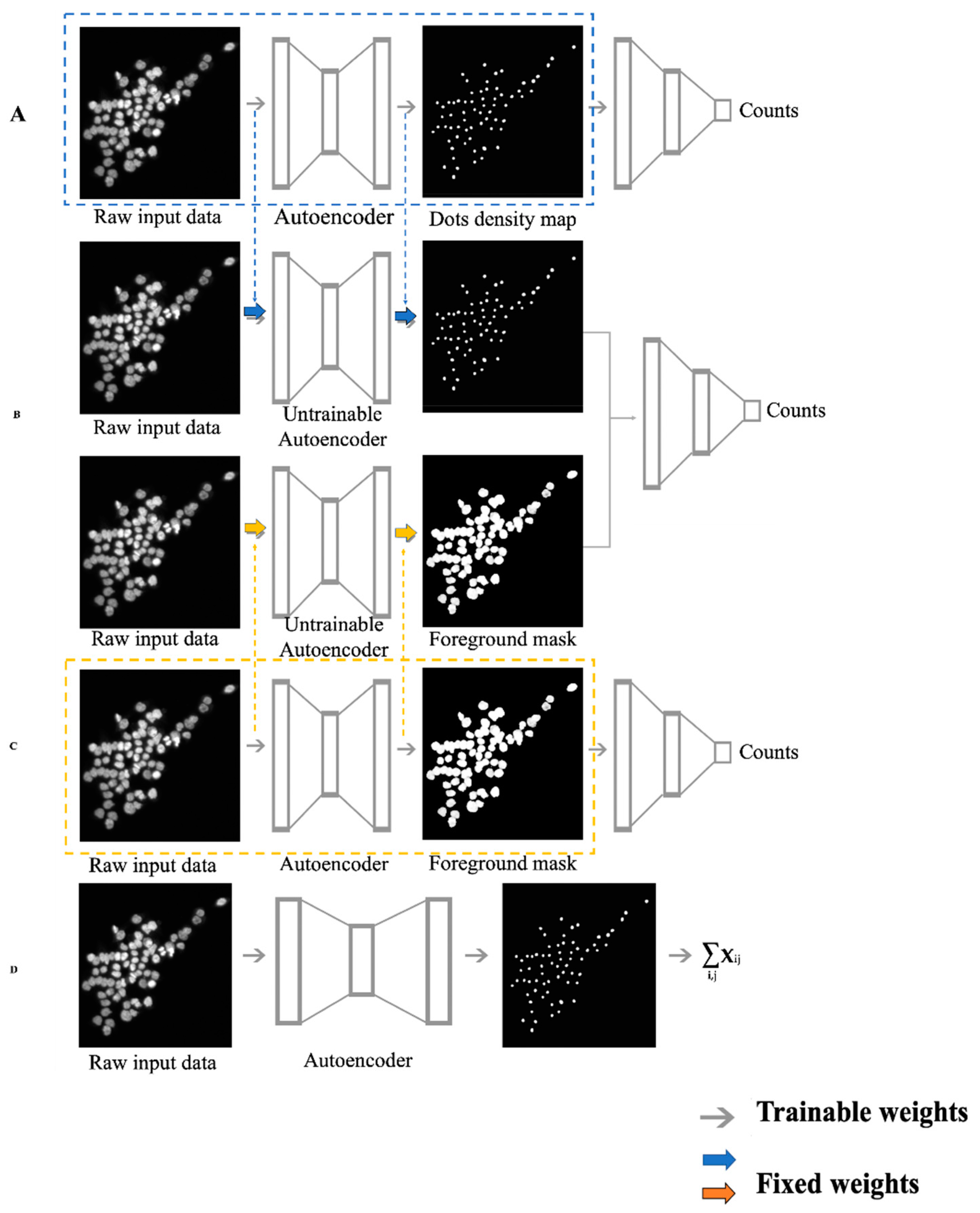
To overcome these challenges, this study introduced a novel model architecture by first extracting both dot density map and foreground mask as imaging features, then stacking the two types of features together using a two-input DCNN model to regress them on the cell counts. This idea came from ensemble learning, which has been well studied and shown to achieve better prediction performance by using multiple learning algorithms [
15,
16,
17]. There are several methods to assemble models; the method used in this study was called stacking learning, which employs a learning algorithm to combine the predictions of other algorithms. Each of these predictions was generated from all training data [
18,
19].
3. Results
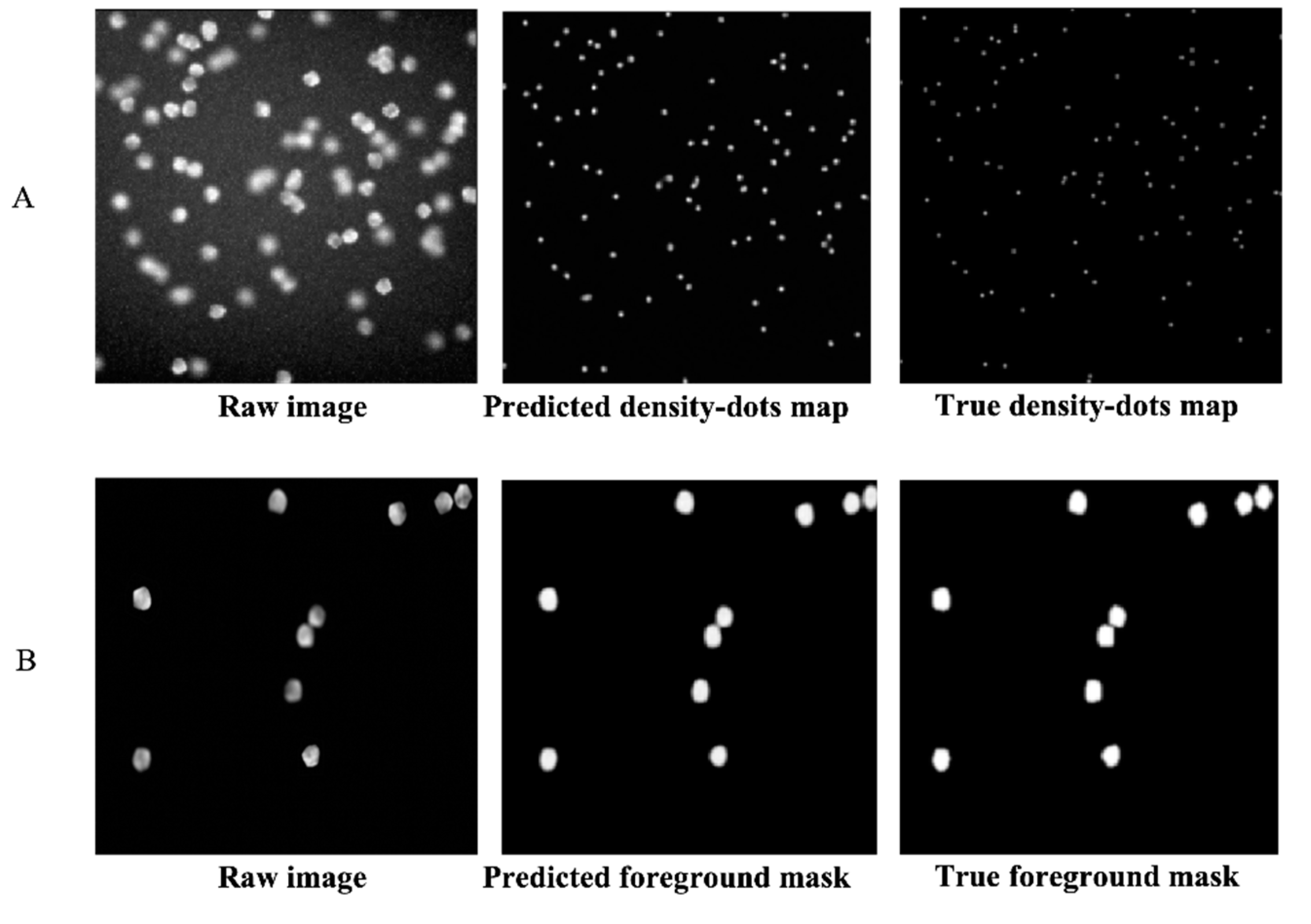
After the first training step of the DRDCNN and FRDCNN (i.e., the training of the autoencoders), predictions were made as to whether the autoencoders could achieve the purpose of feature extraction. The loss of the DRDCNN-based autoencoder was converged to around 0.7, while the loss of the FRDCNN-based autoencoder was converged to around 10.
Figure 2 shows the raw images, predicted features, and the label features (ground truth). Both the predicted dot density map (
Figure 2A) and the predicted foreground mask (
Figure 2B) were quite similar to the true ones. Hence, they had the full ability to represent the features we expected from the raw image data.
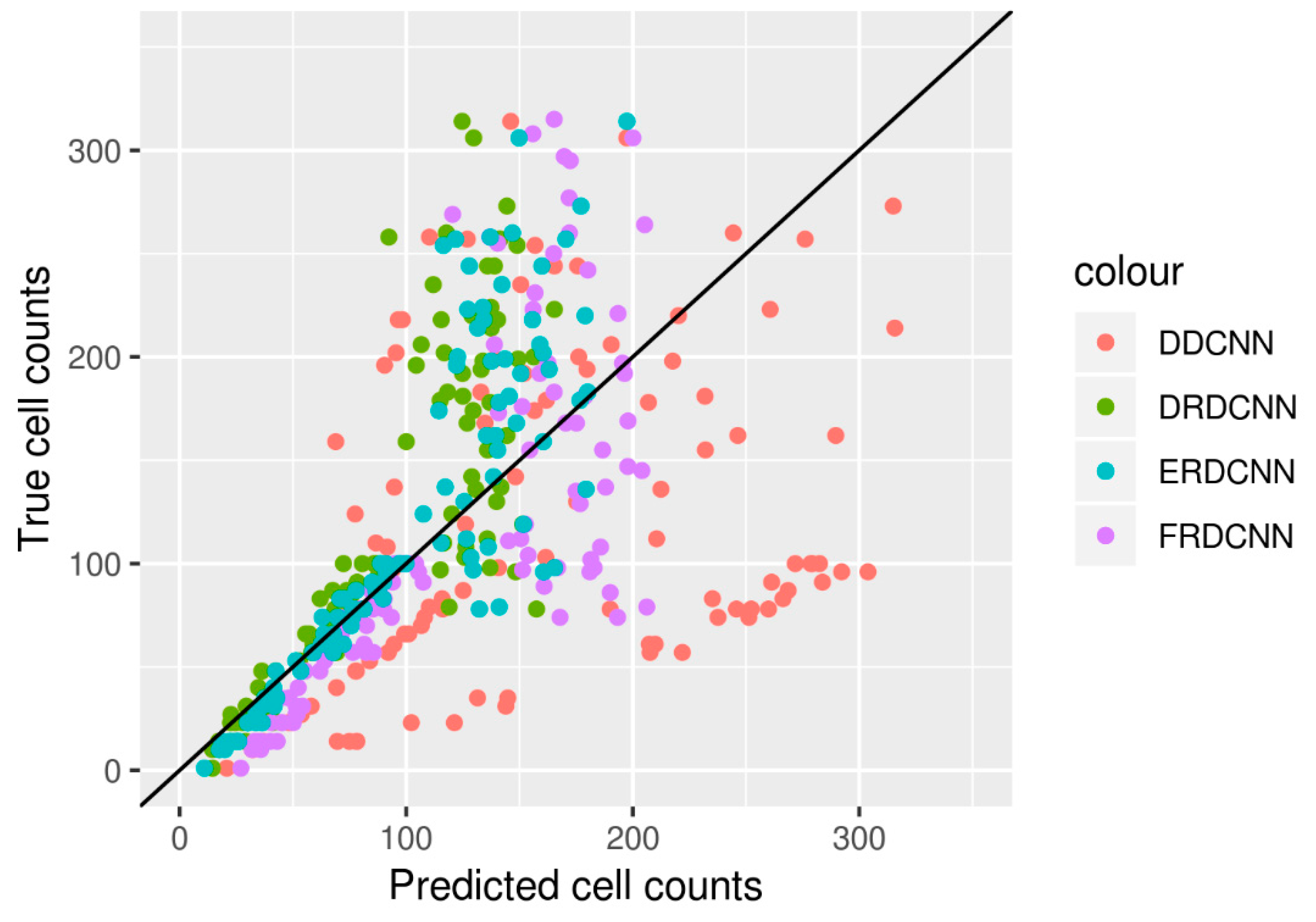
We then evaluated the performance of the four end-to-end DCNN models by predicting the cell counts of the test set with the 100 images. The results are shown in
Table 3, and the three regression-based DCNNs’ predictions (DRDCNN, FRDCNN, and ERDCNN) are further shown in
Figure 3. The proposed ensembling-based regression DCNN model (ERDCNN) had better performance in terms of lower errors (
RMSE = 49.25;
MAE = 31.49) and higher correlation (
r = 0.85).
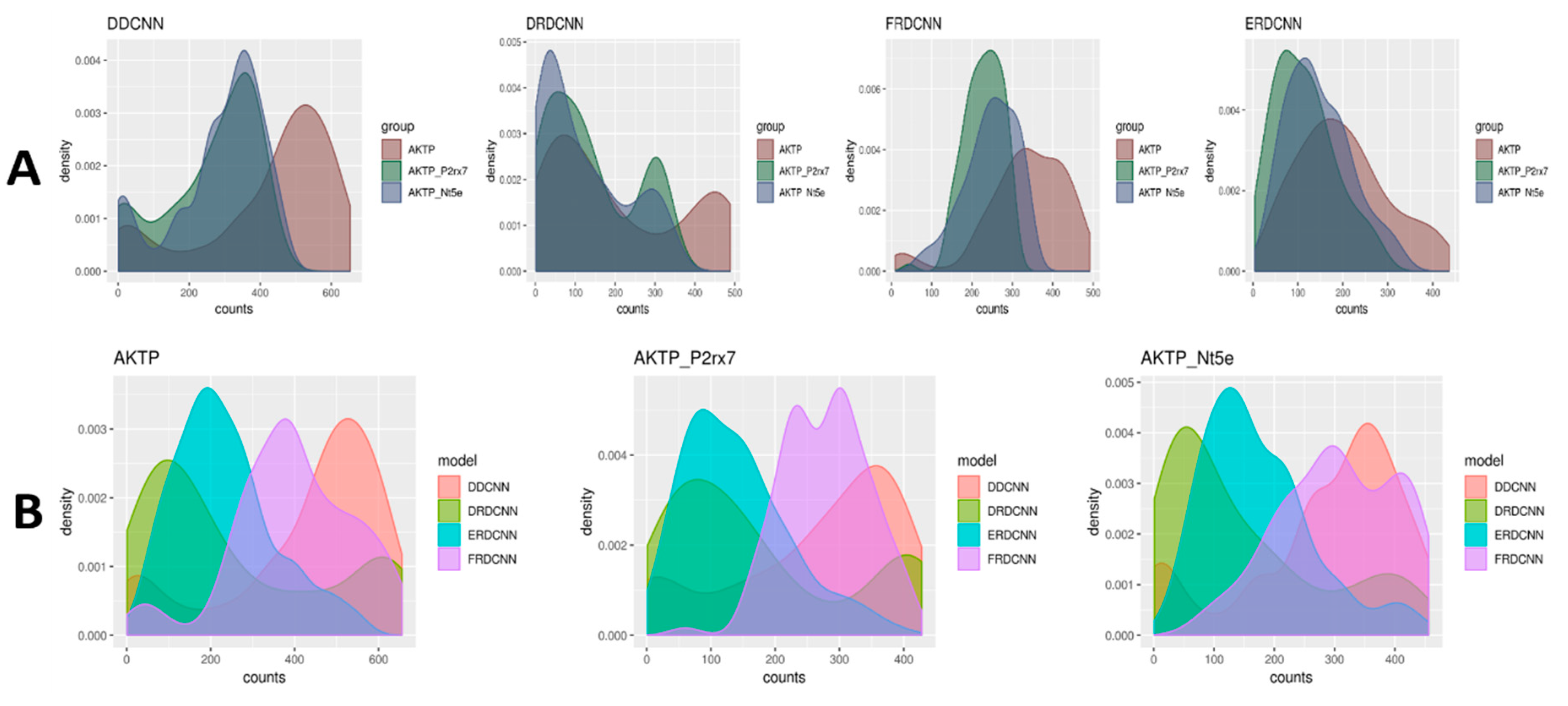
The trained models were used to predict the cell counts for the microscopic images generated from the three experimental groups (where AKTP was the control group, AKTP-P2rx7 and AKTP-Nt5e were the case groups). The t-test results comparing the predicted cell count differences between the control group and the case groups are shown in
Table 4. There was a significant difference of the predicted cell counts between the AKTP-P2rx7 group and the AKTP control group by the ERDCNN and FRDCNN models, where P-values of the ERDCNN, FRDCNN, and DDCNN were 0.0002, 0.002, and 0.009, respectively. The predicted mean cell count by the ERDCNN in the AKTP-P2rx7 group (24.26) was lower than that in the AKTP group (29.69), suggesting that P2rx7 over-expression induced the EMT phenotype in the malignant colorectal cancer organoids and the EMT phenotype inhibited the cell growth of those organoids. However, there was no difference in the predicted cell counts by the ERDCNN between the AKTP-Nt5e group (29.80) and the AKTP group (29.69). A similar conclusion of no significant difference of the predicted cell counts between the AKTP-Nt5e group and the AKTP group was also observed using either the DRDCNN or the FRDCNN model. However, the DDCNN model suggested decreasing cell counts in the AKTP-Nt5e group compared to in the control group (
p-value = 0.03). The distributions of the cell count predictions were very diverse (
Figure 4), which indicated that the models might not be able to predict the exact number of cells in an image from the datasets other than the set under which these models were trained. However, they (e.g., ERDCNN and FRDCNN) were able to predict the overall cell count difference.
4. Discussion
In this study, we developed an integrated end-to-end DCNN model (ERDCNN) to regress microscopic image features to image-specific cell counts. The model integrated the DRDCNN model, which had a U-net as feature extractor, and the weights were initialized from a previous study, and the FRDCNN model, which had a VGG-style autoencoder as feature extractor. Except for the difference in the feature extraction step, the three regression models were quite similar in terms of having a common convolutional regression tail. We also compared the performance of the new model with the published density-only DCNN (DDCNN) model and the two regression-based models (DRDCNN and FRDCNN).
Two synthetic datasets were used in the training and testing procedures. We designed a training strategy by integrating transfer learning of the model weights and ensembling the learned image features. The highest correlation between the true cell counts and the predicted cell counts of the 100 test images was found using the proposed ERDCNN model. The well-trained models were applied to estimate the cell counts of the real microscopic images generated in three experimental conditions. A significant difference of the estimated cell counts was found between one of the two case conditions and the control condition using the proposed model. Although we observed improved performance in our proposed new model (ERDCNN), it took much longer to train the model (1 h for DRDCNN and FRDCNN vs. 5 h for ERDCNN) on a GPU-based Nvidia GeForce GTX 1080 with an 8 GB memory machine.
We observed a major decrease in the performance of the models when the number of cell counts was larger than 100. The major reason for the abnormality was due to the nature of the dataset used in the study. The data were combined from two different data sources, which varied in size, dimension, depth, and, more importantly, cell counts. In one source, the counts ranged from 1 to 100, while in the other source, they ranged from 1 to around 200. The unbalanced distributions of the two dataset sources might have caused the tremendous change of the performance. Another issue might be that the two data sources were generated using different algorithms. To overcome the challenges as much as possible, we did a series of preprocessing, such as resizing, reshaping, and rescaling, to make a combined dataset meeting the requirements of the both branches. The ideal situation would have been to simulate a whole dataset with both density map and foreground mask as labels so that we did not have to combine two datasets together. However, this was outside the scope of this research, and we will explore this issue in more detail in the future.
The model may be improved by incorporating more high-level image features, since our investigation of ensembling two types of image features instead of one type of feature improved the model’s prediction ability. Another limitation of this study was the quality of the data. We only had two synthetic datasets which were generated by different algorithms and had different sizes, dimensions, depths, and, more importantly, cell counts. The cell counts in the images were distributed sparsely. Each cell count category had only one or a few samples, which may be far from enough for a deep regression model like the one we developed here.
In summary, we proposed a strategy to ensemble high-level image features for cell counting, and showed that including more image features would increase the performance and stability of the DCNN model in cell counting.


