Abstract
Although the X chromosome accounts for about 5% of the human genes, it is routinely excluded from genome-wide association studies probably due to its unique structure and complex biological patterns. While some statistical methods have been proposed for testing the association between X chromosomal markers and diseases, very a few of them can adjust for covariates. Unfortunately, those methods that can incorporate covariates either need to specify an X chromosome inactivation model or require the permutation procedure to compute the p value. In this article, we proposed a novel analytic approach based on logistic regression that allows for covariates and does not need to specify the underlying X chromosome inactivation pattern. Simulation studies showed that our proposed method controls the size well and has robust performance in power across various practical scenarios. We applied the proposed method to analyze Graves’ disease data to show its usefulness in practice.
1. Introduction
Many diseases exhibit a gender preference, such as autoimmune diseases, cardiovascular diseases, psychiatric diseases, and cancer, implying that genetic variants on the X chromosome play an important role in sex differences [1,2,3,4,5]. However, most genome-wide association studies (GWAS) routinely exclude the analysis of X-chromosomal variants probably because the X chromosome has a unique structure and complex biological patterns [6,7,8]. Females have one more X chromosome than males, and to balance gene expression on the X chromosome with that of males, one of the female X chromosomes is inactivated in the early embryo [9]. Usually, the process of X chromosome inactivation (XCI) is considered random (XCI-R) [10], i.e., for an X-linked gene, nearly 50% of the cells have the paternal allele active while the rest cells have the maternal allele active. However, studies have shown that skewed XCI (XCI-S) is more biologically plausible [11]. XCI-S is a non-random process, which has been defined as a significant deviation from XCI-R, for instance, the inactivation of one of the alleles in more than 75% of cells [12]. In addition, up to 25% of X-linked genes can escape from XCI (XCI-E) [9]. Both alleles in the genes under XCI-E will be active, which are similar to autosomal genes.
To account for the unique characteristics of the X chromosome, several statistical methods have been developed for testing the association between X chromosomal markers and diseases [13,14,15,16,17,18]. However, very a few of them can adjust for covariates. In large-scale GWAS, spurious associations may occur due to the influence of additional covariates, such as sex, age, and population structure [19,20]. Particularly on the X chromosome, if the sex ratios differ between cases and controls, then sex will be a confounder when the allele frequency of females is unequal to that of males. In practice, a natural way to adjust for covariates is to build a regression model, and logistic regression is generally adopted for binary traits. Based on the logistic regression framework, Gao et al. [15] integrated four tests (, , and ) in the software toolset XWAS. In and , three genotypes of females are both coded by 0, 1, and 2, while two genotypes of males are coded by 0 and 1 for and by 0 and 2 for . In the latter, males are treated as homozygous females to reflect the dosage compensation relationship between the two sexes. Hence, and assume that the underlying XCI patterns are XCI-E and XCI-R, respectively. On the other hand, and build logistic regressions for females and males separately and then combine the two p values using Fisher’s and Stouffer’s methods, respectively. However, these two methods do not take any XCI patterns into consideration and thus may suffer from substantial power loss if the test marker is undergoing XCI. Wang et al. [14] proposed another approach (denoted by ) that can consider four special XCI patterns simultaneously: XCI-R, XCI-E, XCI-S fully toward the normal allele (XCI-SN), and XCI-S fully toward the risk allele (XCI-SR). In their method, three genotypes of females are coded as 0, , and 2 under XCI, where measures the degree of skewness of XCI. For instance, represents that all the risk (normal) alleles are inactivated in heterozygous females, which corresponds to the XCI-SN (XCI-SR) pattern. While has robust performance in power, its p value is evaluated based on the permutation procedure, which is very computationally intensive, especially in GWAS. Hence, it is still desirable to develop a robust method that can both adjust for covariates and analytically calculate the p value.
To fill this gap, this article proposed a novel statistical method to test the association between X chromosomal markers and a specific disease. Our method, which is also based on logistic regression, is robust because it does not require assigning a specific XCI pattern. Further, our method can compute the p value without the resample procedure by directly using the rhombus formula. We implemented an extensive simulation study to compare the performance of our approach with the existing ones. Simulation results showed that our method controls the size well and can maintain relatively high power across a variety of scenarios. Finally, we applied our proposed approach to the Graves’s disease data to demonstrate its practical use.
2. Method
Consider an X-linked SNP with deleterious allele A and normal allele a. Then, there are three possible genotypes for females: aa, Aa, and AA, and two for males: a and A. We assume a binary variable for the disease of interest with representing individuals with (without) the disease. denotes the covariates that need to be adjusted in the model, where is the model intercept and represents the binary variable with 1 being female and 0 being male. We further assume that the relationship between the phenotype and genotype for individual can be constructed by the following logistic regression model:
where the subscript denotes the th individual, is the genotypic score, and represents the regression coefficients for the covariates and the genotypic score. Note that the genotypic score depends on the underlying XCI pattern. According to the coding strategy by Wang et al. [14], can be written in the following uniform form
where is the indicator function, and and are unknown parameters depending on the underlying XCI pattern. For instance, when the SNP is undergoing XCI, and can be assigned by and 2, respectively. In this coding strategy, is a measure of the skewness of XCI, and males are treated as homozygous females to reflect the dosage compensation. Table 1 lists the genotypic scores for all five genotypes and the corresponding values of and under the four special XCI patterns.

Table 1.
The genotypic scores for five genotypes and their corresponding values of and under the four special XCI patterns.
We chose the score statistic to test the null hypothesis: because the association tests for all the SNPs share the same null model. For a total sample size of , the score function can be derived as
where is the disease probability estimated for individual without considering the genotype (details of the derivation are given in Appendix A). The information matrix of (1) can be written as follows:
where
and
Under the null hypothesis: , we have
where is estimated as the variance of . Therefore, the statistic
asymptotically follows a standard normal distribution under the null hypothesis.
Note that the calculation of the test statistic relies on the underlying XCI pattern. Unfortunately, this is generally unknown for a specific SNP. We thereby proposed a robust test referred to as to account for the four special XCI models. The statistic is defined as follows:
Due to the correlation between the four score tests, does not follow any classical distributions. We assume that , , , and jointly asymptotically follow a multivariate normal distribution , where is a four-dimensional vector with all elements being 0, and is the correlation matrix with
In the above correlation matrix, is the correlation coefficient between and . Given , we can analytically derive the p value of . Particularly, let be the density function of the multivariate normal distribution then, for a given , the p value of is calculated by
Next, we need to accurately estimate the correlation matrix . To this end, we first build a new model that contains two parameters representing genetic effects as follows:
The information matrix of (2) can be expressed as follows:
where
and
Under the null hypothesis , the statistic
asymptotically follows a chi-square distribution with two degrees of freedom, where
is the covariance matrix of and . Therefore, the correlation coefficient between and can be estimated as
Once is estimated, we can calculate the p value of . Although the four-dimensional integral can be calculated in the commonly used software (e.g., the mvtnorm package in R, https://cran.r-project.org/web/packages/mvtnorm/index.html, (accessed on 10 April 2022)), the algorithm based on the Quasi-Monte-Carlo procedure needs a lot of computing resources to achieve relatively high accuracy. Hence, it would be still desirable to obtain its analytic form if possible. Fortunately, we can use the rhombus formula [13,21] to obtain the upper bound of the p-value of as follows:
where and denote the cumulative distribution function and probability density function of the standard normal distribution, respectively, and , where is the correlation efficient between th and th score statistics. Note the order of four test statistics , , and is not specified in the above formula, so 12 kinds of upper bounds can be obtained. Therefore, only the smallest bound among them is adopted as an approximation of the p value. As shown in Wang et al. [13], such approximation is very accurate for small p values, which would be quite useful in GWAS because the significance level is generally very stringent (e.g., ) in such studies.
3. Simulation Study
3.1. Simulation Settings
We conducted comprehensive simulation studies to compare the performance of with , , , and , all of which can adjust covariates. Note that we did not include the in our simulations because this method is a permutation-based approach, which would be too time-consuming for GWAS. The data are simulated from the following model:
where is the binary covariate sex, is a continuous covariate, which is sampled from the uniform distribution and is the genotype score. The ratio of males to females is assumed to be in the general population, so follows a binomial distribution . Further, we assume that the genotype of females (aa, Aa, AA) follows a trinomial distribution with probabilities , while the genotype of males (a, A) follows a binomial distribution . Let and be the respective risk allele frequency and the inbreeding coefficient for females. Then, we have , , and . The values of and are both set to be 0.1, 0.2, and 0.3, so there are nine combinations in total. is assigned to be 0 and 0.05, where the former implies Hardy–Weinberg equilibrium (HWE) and the latter represents a scenario of Hardy–Weinberg disequilibrium (HWD). The intercept is fixed at . For the coefficients and , we consider two cases for each of them: and . The genetic effect is set to be 0, 0.1116, 0.15, and 0.1858, where means no association between the SNP and the disease status, and the other three values of indicate that the odds ratios of females with genotype AA are about 1.25, 1.35, and 1.45. Obviously, the case of is used to study the size, while the empirical power is investigated in the non-zero cases.
Note that, when studying the power, we only choose three combinations of and : for convenience. The scenarios that the SNP undergoes XCI or escapes from XCI are both considered. For the former, we let range from 0 to 2 in increments of 0.5. As such, we have considered various XCI patterns, including XCI-SN, XCI-R, and XCI-SR. Once the XCI pattern is assumed, we can assign the corresponding value for the genotypic score .
Given the covariates, the genotypic score, and the regression coefficients, we can generate the disease status from the binomial distribution for a large population. Then, we randomly sample 2500 cases and 2500 controls from this population. We find that when , the proportions of females in cases varied from 40% to 60% in the simulated data. The size is estimated at three nominal levels: based on 1,000,000 replicates, while the power is only estimated at the nominal level based on 10,000 replicates. The p value of is evaluated by using the rhombus formula.
3.2. Results
3.2.1. Size
Table 2 shows the estimated type I error rate at the nominal significance level when HWE holds in the female population. As expected, all the methods controlled the size well in all the scenarios. Although appears slightly conservative in some scenarios, its p values are similar to the nominal level. We also simulated the scenarios of HWD (). However, we observed that the performances of all the tests were similar to those of Table 2, and HWD in females had little impact on the size. Therefore, the simulation results with non-zero are presented in the Supplementary Material (Table S1). The results of type I error rates estimated at the nominal level and are also given in Supplementary Material (Tables S2–S5). As can be seen, XCMAX4 still had the correct size in general, except being slightly conservative at .
Table 2.
Estimated type I error rate at the nominal significance level for , , , , and against , , , and based on 1,000,000 replicates under HWE.
3.2.2. Power
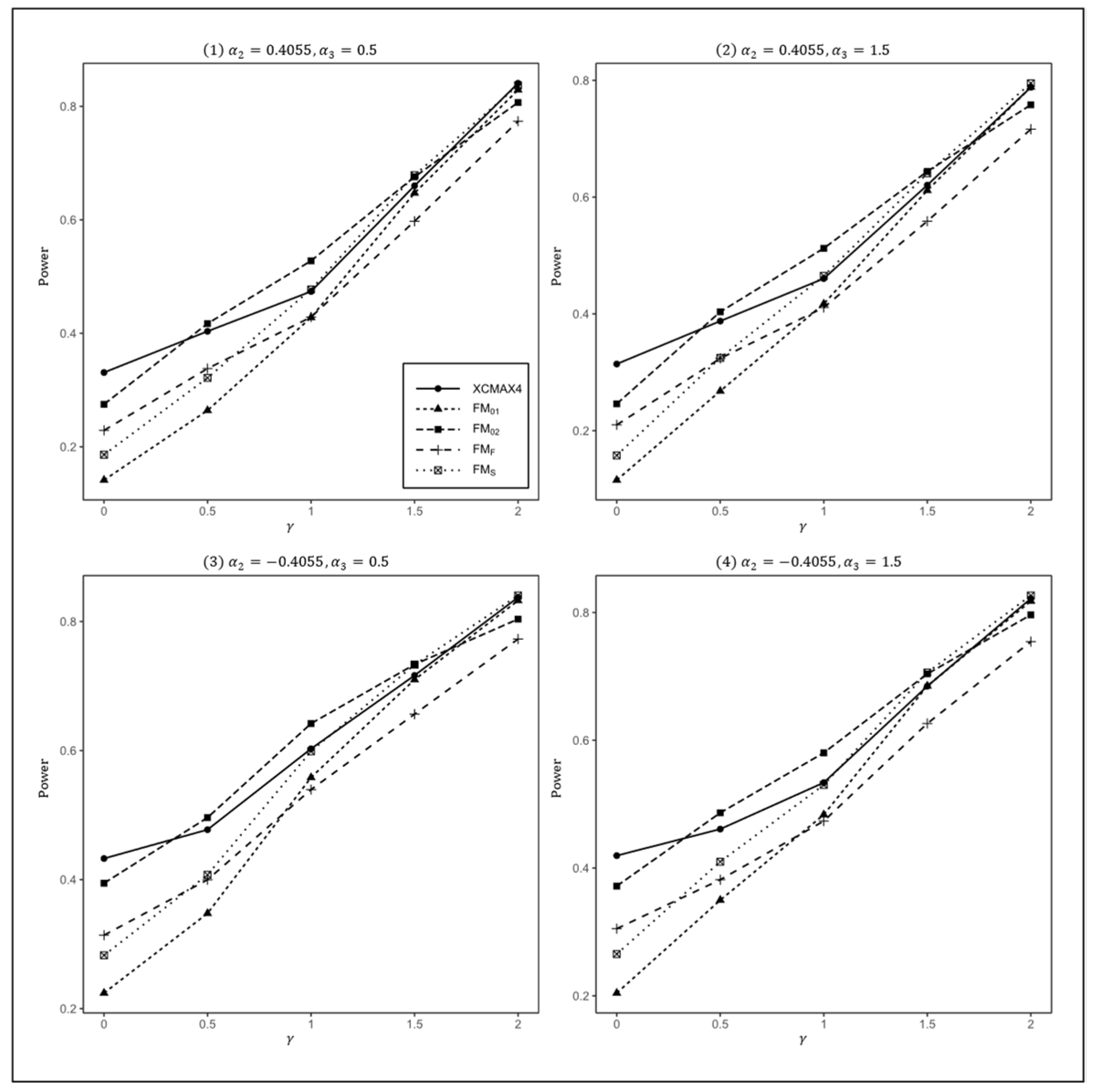
Figure 1, Figure 2 and Figure 3 plot the powers of , , , , and under various XCI patterns when , and , and respectively. These figures show that all four subfigures exhibited a similar pattern in power, indicating that the covariates had a very limited impact on the performance of all methods.

Figure 1.
Estimated powers of , , , , and under various XCI models. The simulation was based on 10,000 replicates with , , , and .
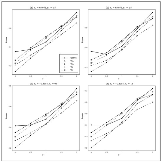
Figure 2.
Estimated powers of , , , , and under various XCI models. The simulation was based on 10,000 replicates with , , , , and .
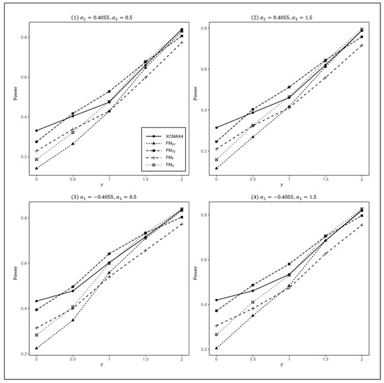
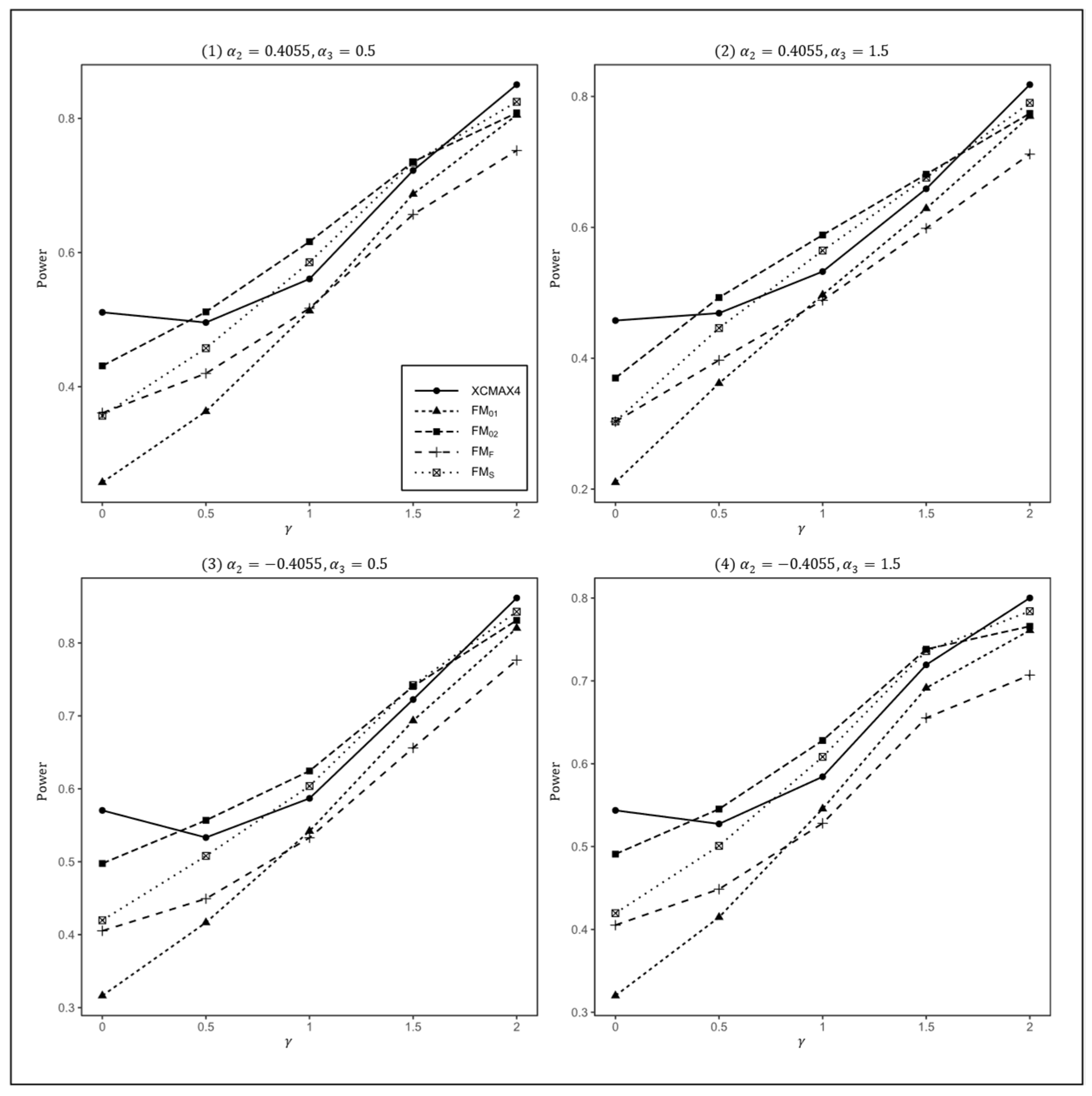
Figure 3.
Estimated powers of , , , , and under various XCI models. The simulation was based on 10,000 replicates with , , , , and .
In Figure 1, we can see that and were generally less powerful than other methods in all situations. performed best when (XCI-SN) and 2 (XCI-SR). However, when (XCI-R), was the most powerful, followed by and . This was expected because is proposed exactly under XCI-R. We also observed that had a better power than when , while performed slightly better than when . In both scenarios, was still the most powerful method, but the differences in power between these three methods were generally very small. Notice that the results in Figure 2 and Figure 3 are analogous to those in Figure 1, and thereby the allele frequencies of females and males did not apparently change the power profiles of all of the methods.
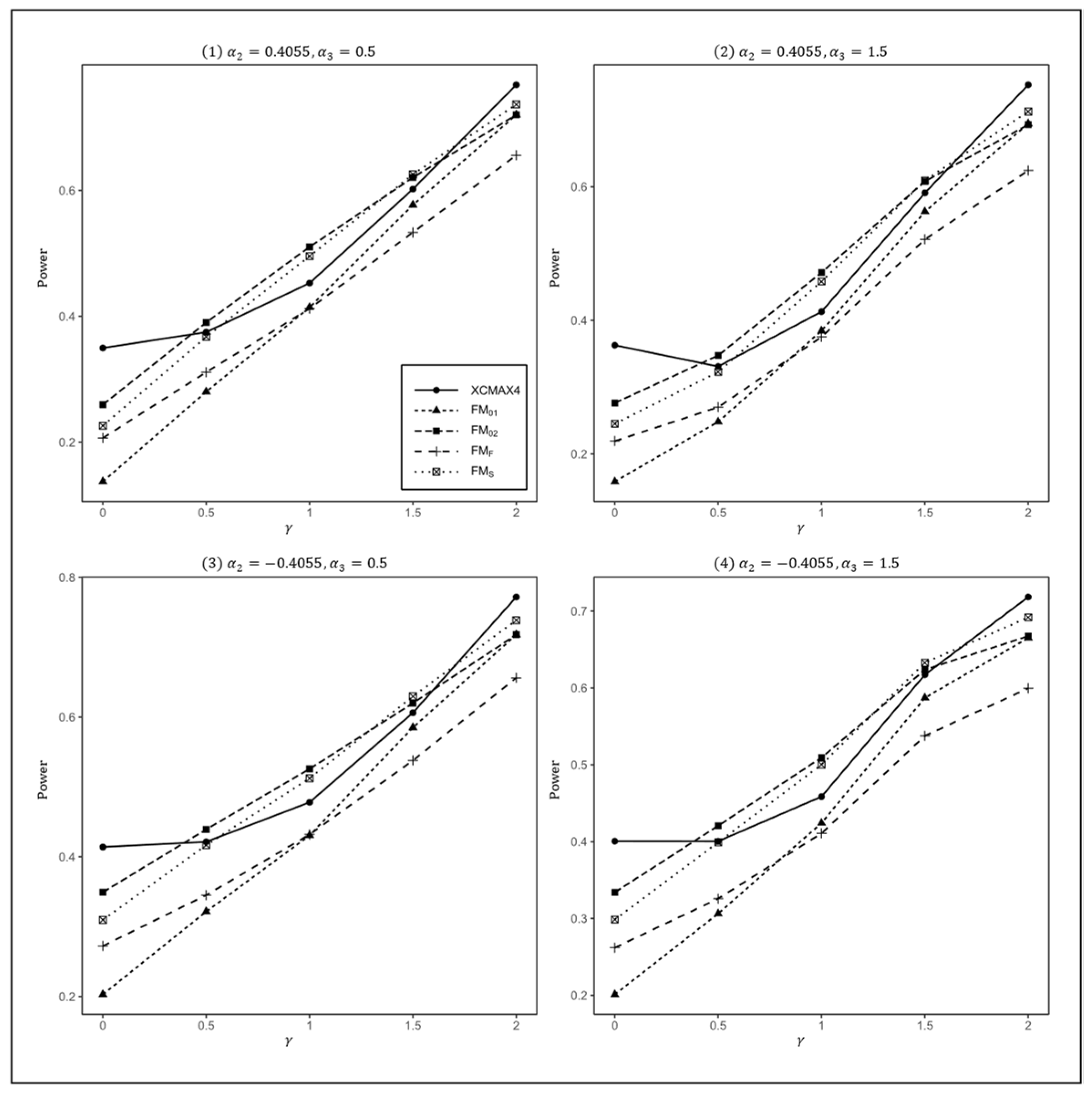
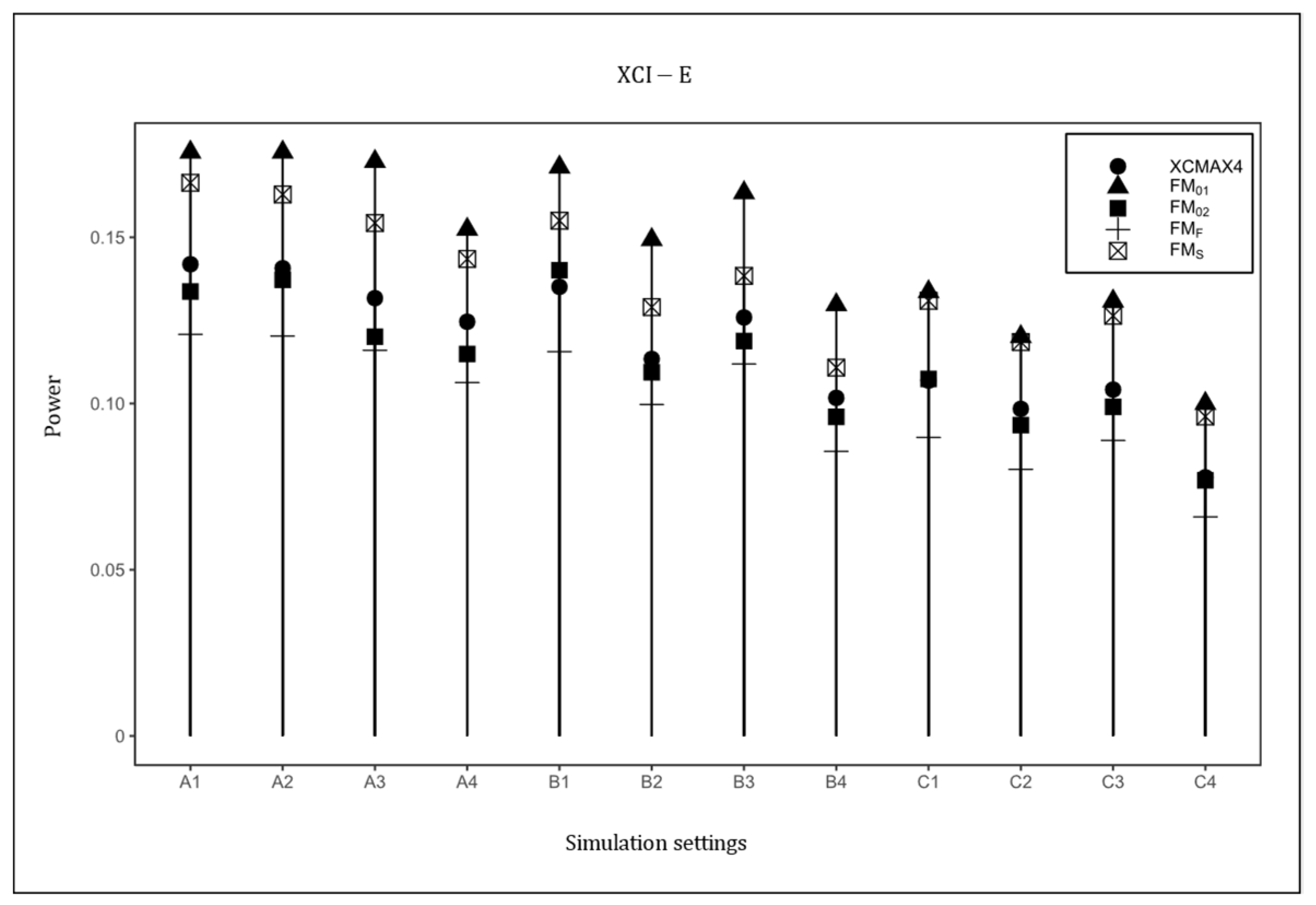
Figure 4 plots the powers of , , , , and under the XCI-E pattern with . Based on this figure, was uniformly the most powerful in all scenarios as expected, followed by and . was generally less powerful than , , and , but still performed better than . The power results with , and are provided in Supplementary Material (Figures S1–S4), which are similar to those in Figure 1, Figure 2, Figure 3 and Figure 4, indicating that HWD in females had little effect on the power results. The power results with are generally consistent with those in Figure 1, Figure 2, Figure 3 and Figure 4, implying that the properties of did not vary with the magnitude of the genetic effect (see Figures S5–S20 in Supplementary Material). As expected, when the value of increased, the powers of all methods uniformly increased.

Figure 4.
Powers of , , , , and under XCI-E. The simulation was based on 10,000 replicates with , , and . In the horizontal coordinates, “A”, “B”, and “C” represent three combinations of : , , and , respectively, and the numbers 1–4 represent four combinations of : , , , and , respectively.
In conclusion, and can have high power if the underlying XCI pattern is modelled correctly but may be less powerful in other scenarios. In contrast, retained a relatively good power across a variety of scenarios. Compared to , may suffer from power loss if the SNP is undergoing XCI but will be more powerful under XCI-E. had the overall worst performance and thus is not recommend. It should be noted that, , , , and adopted logistic regression, which is slightly more computationally intensive than in GWAS because the implementation of the logistic regression requires additional iterations. Compared to the other four methods, testing 2000 SNPs, saved half the time. The details of time comparisons are given in Supplemental Material (Table S6).
4. Application to Graves’ Disease Data
Graves’ disease (GD) is an autoimmune disease of hyperthyroidism that is four times more common in women than in men [22,23]. Substantial studies have shown that the genetic background explains about four-fifths of the susceptibility to GD.
Considering the distinct gender bias, it is highly reasonable to speculate that the genes on the X chromosome play an important role in the development of GD. Recently, two independent studies found that rs3827440, a non-synonymous SNP of the GRP174 gene on the X chromosome, was associated with GD. A two-stage GWAS, focused on the Han population in China, first reported this finding, which was further validated in two Caucasian cohorts. There are two alleles at rs3827400, with T being the risk allele and C being the normal one. Table 3 displays the four datasets about rs3827400 mentioned in these two studies. We applied , , , , and to each dataset; the results are shown in Table 4. Note that sex was included as a covariate when calculating the p values of , , and .
Table 3.
Data of rs3827400 related to Graves’ disease in two independent studies.
Table 4.
p values of the , , , , and tests from four datasets.
This table indicates that none of these methods uniformly performed the best across all four datasets. For the two datasets from the Chinese population, all methods consistently showed that rs3827400 was associated with GD at the . Among these tests, consistently had the second smallest p values. However, the p values of all the methods from both Caucasian datasets suggested no such an association at the same significance level probably because of their relatively small sample size. We also observed that appeared slightly conservative in these scenarios, but this was not surprising because the rhombus formula is less accurate when the p value is greater than 0.01.
Because both the Han population and the Caucasian population contained two datasets, we also tested such association at the population level by treating the data source as an additional covariate. The corresponding results are given in Table 5, which are similar to those in Table 4.
Table 5.
p values of , , , , and tests from Han and Caucasian populations.
5. Discussion
This paper proposed a novel robust method, , to test the association between the marker on the X chromosome and a specific disease for case-control design. Our method is an extension of the [24] test on the X chromosome, which can both incorporate the information of XCI and allow for covariates. Unlike the proposed by Wang et al., is construted by using the score test, which is more efficient in GWAS because we only need to fit the null model once. Moreover, the requires permutation to calculate the p value, which makes it unappealing in GWAS. In contrast, the p value of can be computed analytically by using the rhombus formula. On the other hand, although , , , and can also adjust for covariates, they do not take various XCI models into consideration and thus may suffer from substantial power loss in some scenarios. However, can retain a relatively high power by accounting for four special XCI patterns simultaneously. Simulation results showed that controlled the size well and had robust performance in power. Therefore, we recommend using for its effectiveness, robustness, and generality. Finally, to help implement in practice, we provide an R function , which is available at https://github.com/YoupengSU/XCMAX4.git (accessed on 12 April 2022).
Supplementary Materials
The following supporting information can be downloaded at: https://www.mdpi.com/article/10.3390/genes13050847/s1, Table S1: Estimated typeⅠerror rate at the nominal significance level for , , , , and against , , , and based on 1,000,000 replicates when .; Tables S2–S5: Estimated typeⅠerror rates at the nominal significance levels and ; Table S6: Time used to test 2000 SNPs with a sample size of 5000; Figures S1–S4: Powers of , , , , and when ; Figures S5–S20: Powers of , , , , and when .
Author Contributions
Conceptualization, P.W. and Y.S.; methodology, Y.S.; validation, P.W. and J.H.; formal analysis, Y.S. and J.H.; writing—original draft, Y.S. and J.H.; writing—review and editing, P.W. and J.H.; visualization S.C., Z.C., and M.D.; supervision, P.W.; funding acquisition, P.Y. and H.J. All authors have read and agreed to the published version of the manuscript.
Funding
The study was supported by the National Natural Science Foundation of China (No. 82173628) and the National Key R&D Program of China (No. 2018YFE0206900).
Institutional Review Board Statement
Not applicable.
Informed Consent Statement
Informed consent was obtained from all subjects involved in the study.
Data Availability Statement
The real data used in this study are available from two published papers at https://dx.doi.org/10.1136%2Fjmedgenet-2013-101595, and https://doi.org/10.1111/tan.12259 (assessed on 7 April 2022).
Conflicts of Interest
The authors declare no conflict of interest.
Appendix A. Detailed Derivation of the Score Statistic
The log-likelihood function of Model (1) can be written as
where representing the probability of having disease for th individual.
Assume that is the restricted maximum likelihood estimate of under the condition , then the score function and Fisher’s information matrix can be given as
and
where
and
By Cox et. al. [25], we can obtain the score test statistic as
which asymptotically follows a chi-square distribution with degrees of freedom being 1. In Model (2), β becomes a two-dimensional vector, and the proofs are similar, so the details are omitted.
References
- Voskuhl, R. Sex differences in autoimmune diseases. Biol. Sex Differ. 2011, 2, 1. [Google Scholar] [CrossRef] [Green Version]
- Appelman, Y.; van Rijn, B.B.; Ten Haaf, M.E.; Boersma, E.; Peters, S.A. Sex differences in cardiovascular risk factors and disease prevention. Atherosclerosis 2015, 241, 211–218. [Google Scholar] [CrossRef]
- Riecher-Rossler, A. Sex and gender differences in mental disorders. Lancet Psychiatry 2017, 4, 8–9. [Google Scholar] [CrossRef]
- Dong, M.; Cioffi, G.; Wang, J.; Waite, K.A.; Ostrom, Q.T.; Kruchko, C.; Lathia, J.D.; Rubin, J.B.; Berens, M.E.; Connor, J.; et al. Sex Differences in Cancer Incidence and Survival: A Pan-Cancer Analysis. Cancer Epidemiol. Biomark. Prev. 2020, 29, 1389–1397. [Google Scholar] [CrossRef] [PubMed]
- Erol, A.; Winham, S.J.; McElroy, S.L.; Frye, M.A.; Prieto, M.L.; Cuellar-Barboza, A.B.; Fuentes, M.; Geske, J.; Mori, N.; Biernacka, J.M.; et al. Sex differences in the risk of rapid cycling and other indicators of adverse illness course in patients with bipolar I and II disorder. Bipolar Disord. 2015, 17, 670–676. [Google Scholar] [CrossRef] [PubMed]
- Lu, Z.; Carter, A.C.; Chang, H.Y. Mechanistic insights in X-chromosome inactivation. Philos. Trans. R Soc. Lond. B Biol. Sci. 2017, 372, 356. [Google Scholar] [CrossRef] [PubMed]
- Lyon, M.F. Gene action in the X-chromosome of the mouse (Mus musculus L.). Nature 1961, 190, 372–373. [Google Scholar] [CrossRef] [PubMed]
- Carrel, L.; Willard, H.F. X-inactivation profile reveals extensive variability in X-linked gene expression in females. Nature 2005, 434, 400–404. [Google Scholar] [CrossRef] [PubMed]
- Fang, H.; Disteche, C.M.; Berletch, J.B. X Inactivation and Escape: Epigenetic and Structural Features. Front. Cell Dev. Biol. 2019, 7, 219. [Google Scholar] [CrossRef]
- Disteche, C.M. Dosage compensation of the sex chromosomes and autosomes. Semin. Cell Dev. Biol. 2016, 56, 9–18. [Google Scholar] [CrossRef] [Green Version]
- Cantone, I.; Fisher, A.G. Human X chromosome inactivation and reactivation: Implications for cell reprogramming and disease. Philos. Trans. R Soc. Lond. B Biol. Sci. 2017, 372, 358. [Google Scholar] [CrossRef] [PubMed]
- Wang, P.; Zhang, Y.; Wang, B.Q.; Li, J.L.; Wang, Y.X.; Pan, D.; Wu, X.B.; Fung, W.K.; Zhou, J.Y. A statistical measure for the skewness of X chromosome inactivation based on case-control design. BMC Bioinform. 2019, 20, 11. [Google Scholar] [CrossRef] [PubMed]
- Wang, P.; Xu, S.Q.; Wang, B.Q.; Fung, W.K.; Zhou, J.Y. A robust and powerful test for case-control genetic association study on X chromosome. Stat. Methods Med. Res. 2019, 28, 3260–3272. [Google Scholar] [CrossRef] [PubMed]
- Wang, J.; Yu, R.; Shete, S. X-chromosome genetic association test accounting for X-inactivation, skewed X-inactivation, and escape from X-inactivation. Genet. Epidemiol. 2014, 38, 483–493. [Google Scholar] [CrossRef]
- Gao, F.; Chang, D.; Biddanda, A.; Ma, L.; Guo, Y.; Zhou, Z.; Keinan, A. XWAS: A Software Toolset for Genetic Data Analysis and Association Studies of the X Chromosome. J. Hered. 2015, 106, 666–671. [Google Scholar] [CrossRef] [Green Version]
- Clayton, D. Testing for association on the X chromosome. Biostatistics 2008, 9, 593–600. [Google Scholar] [CrossRef]
- Zheng, G.; Joo, J.; Zhang, C.; Geller, N.L. Testing association for markers on the X chromosome. Genet. Epidemiol. 2007, 31, 834–843. [Google Scholar] [CrossRef]
- Chen, Z.; Ng, H.K.; Li, J.; Liu, Q.; Huang, H. Detecting associated single-nucleotide polymorphisms on the X chromosome in case control genome-wide association studies. Stat. Methods Med. Res. 2017, 26, 567–582. [Google Scholar] [CrossRef]
- Clayton, D.G. Sex chromosomes and genetic association studies. Genome Med. 2009, 1, 110. [Google Scholar] [CrossRef] [Green Version]
- Price, A.L.; Patterson, N.J.; Plenge, R.M.; Weinblatt, M.E.; Shadick, N.A.; Reich, D. Principal components analysis corrects for stratification in genome-wide association studies. Nat. Genet. 2006, 38, 904–909. [Google Scholar] [CrossRef]
- Li, Q.Z.; Zheng, G.; Li, Z.H.; Yu, K. Efficient approximation of P-value of the maximum of correlated tests, with applications to genome-wide association studies. Ann. Hum. Genet. 2008, 72, 397–406. [Google Scholar] [CrossRef] [PubMed]
- Chu, X.; Shen, M.; Xie, F.; Miao, X.J.; Shou, W.H.; Liu, L.; Yang, P.P.; Bai, Y.N.; Zhang, K.Y.; Yang, L.; et al. An X chromosome-wide association analysis identifies variants in GPR174 as a risk factor for Graves’ disease. J. Med. Genet. 2013, 50, 479–485. [Google Scholar] [CrossRef] [PubMed] [Green Version]
- Szymanski, K.; Miskiewicz, P.; Pirko, K.; Jurecka-Lubieniecka, B.; Kula, D.; Hasse-Lazar, K.; Krajewski, P.; Bednarczuk, T.; Ploski, R. rs3827440, a nonsynonymous single nucleotide polymorphism within GPR174 gene in X chromosome, is associated with Graves’ disease in Polish Caucasian population. Tissue Antigens 2014, 83, 41–44. [Google Scholar] [CrossRef] [PubMed]
- Chen, Z.; Zang, Y. CMAX3: A Robust Statistical Test for Genetic Association Accounting for Covariates. Genes 2021, 12, 1723. [Google Scholar] [CrossRef]
- Cox, D.R.; Hinkley, D.V. Theoretical Statistics; CRC Press: Boca Raton, FL, USA, 1979. [Google Scholar]
Publisher’s Note: MDPI stays neutral with regard to jurisdictional claims in published maps and institutional affiliations. |
© 2022 by the authors. Licensee MDPI, Basel, Switzerland. This article is an open access article distributed under the terms and conditions of the Creative Commons Attribution (CC BY) license (https://creativecommons.org/licenses/by/4.0/).