
Improving the Utilization of STRmix™ Variance Parameters as Semi-Quantitative Profile Modeling Metrics


Abstract
1. Introduction
2. Materials and Methods
2.1. Construction, Amplification, Capillary Electrophoresis, and Analysis of Unchallenged DNA Samples
2.2. Construction, Amplification, CE, and Analysis of Challenged DNA Samples

| Study | Number of Samples | Input Amounts | Replicate Amplifications | Replicate STRmix Interpretations |
|---|---|---|---|---|
| Single-source, nominal-input | 14 | 2 ng | 1 | 10 |
| Single-source dilution series (higher level) | 2 | 8 ng, 4 ng, 2 ng, 1 ng, 500 pg, 250 pg | 2 | 1 |
| Single-source dilution series (lower level) | 2 | 125 pg, 63 pg | 4 | 1 |
| Donor Number (Donor Set) | Mixture Ratio | Input Amounts | Replicate Amplifications |
|---|---|---|---|
| 2-person (set 1) | 9:1 | 2 ng, 1 ng, 870 pg, 750 pg, 500 pg, 380 pg, 250 pg, 125 pg, 63 pg | 2 |
| 2-person (set 1) | 49:1 | 2.5 ng, 1.9 ng, 1.25 ng, 625 pg, 313 pg | 2 |
| 2-person (set 1) | 99:1 | 2.5 ng, 1.25 ng, 625 pg | 2 |
| 2-person (set 2) | 1:1 | 800 pg, 400 pg, 200 pg, 100 pg, 50 pg, 25 pg | 1 |
| 2-person (set 2) | 3:1 | 800 pg, 400 pg, 348 pg, 300 pg, 200 pg, 152 pg, 100 pg, 50 pg, 25 pg | 1 |
| 3-person (set 1) | 3:2:1 | 1.2 ng, 600 pg, 522 pg, 450 pg, 300 pg, 228 pg, 150 pg, 75 pg, 38 pg | 2 |
| 3-person (set 1) | 10:5:1 | 3.2 ng, 1.6 ng, 1.4 ng, 1.2 ng, 800 pg, 608 pg, 400 pg, 200 pg, 100 pg | 2 |
| 3-person (set 1) | 100:100:4 | 1.28 ng, 625 pg, 325 pg | 2 |
| 3-person (set 2) | 1:1:1 | 1.2 ng, 600 pg, 300 pg, 150 pg, 75 pg, 38 pg | 1 |
| 3-person (set 2) | 3:2:1 | 1.2 ng, 522 pg, 300 pg, 150 pg, 38 pg | 2 |
| 3-person (set 2) | 10:5:1 | 3.2 ng, 1.4 ng, 800 pg, 400 pg, 100 pg | 2 |
| 3-person (set 2) | 100:100:4 | 1.28 ng, 638 pg, 319 pg | 2 |
| 4-person (set 1) | 4:3:2:1 | 2 ng, 1 ng, 870 pg, 750 pg, 500 pg, 380 pg, 250 pg, 125 pg, 63 pg | 2 |
| 4-person (set 1) | 10:5:2:1 | 3.6 ng, 1.8 ng, 1.6 ng, 1.4 ng, 900 pg, 684 pg, 450 pg, 225 pg, 113 pg | 2 |
| 4-person (set 1) | 100:100:100:6 | 1.28 ng, 625 pg, 325 pg | 2 |
| 4-person (set 2) | 1:1:1:1 | 1.6 ng, 800 pg, 400 pg, 200 pg, 100 pg, 50 pg | 1 |
| 4-person (set 2) | 4:3:2:1 | 2 ng, 870 pg, 500 pg, 250 pg, 63 pg | 2 |
| 4-person (set 2) | 10:5:2:1 | 3.6 ng, 1.6 ng, 900 pg, 450 pg, 113 pg | 2 |
| 4-person (set 2) | 100:100:100:6 | 1.28 ng, 638 pg, 319 pg | 2 |
| Donor Number | Mixture Ratio | Treatment |
|---|---|---|
| 2-person | 3:1 | Hematin: 400 µM, 475 µM, 550 µM, 625 µM, 700 µM |
| 10:1 | Hematin: 400 µM, 475 µM, 550 µM, 625 µM, 700 µM | |
| 3:1 | Humic acid: 200 ng/µL, 250 ng/µL, 300 ng/µL, 350 ng/µL, 400 ng/µL | |
| 10:1 | Humic acid: 200 ng/µL, 250 ng/µL, 300 ng/µL, 350 ng/µL, 400 ng/µL | |
| 3-person | 3:2:1 | Hematin: 400 µM, 475 µM, 550 µM, 625 µM, 700 µM |
| 10:5:1 | Hematin: 400 µM, 475 µM, 550 µM, 625 µM, 700 µM | |
| 3:2:1 | Humic acid: 200 ng/µL, 250 ng/µL, 300 ng/µL, 350 ng/µL, 400 ng/µL | |
| 10:5:1 | Humic acid: 200 ng/µL, 250 ng/µL, 300 ng/µL, 350 ng/µL, 400 ng/µL | |
| 4-person | 4:3:2:1 | Hematin: 400 µM, 475 µM, 550 µM, 625 µM, 700 µM |
| 10:5:2:1 | Hematin: 400 µM, 475 µM, 550 µM, 625 µM, 700 µM | |
| 4:3:2:1 | Humic acid: 200 ng/µL, 250 ng/µL, 300 ng/µL, 350 ng/µL, 400 ng/µL | |
| 10:5:2:1 | Humic acid: 200 ng/µL, 250 ng/µL, 300 ng/µL, 350 ng/µL, 400 ng/µL |
| Dry Heat Treatment Number | Dry Heat Exposure Time |
|---|---|
| 1 | 5.75 h |
| 2 | 12.13 h |
| 3 | 19.42 h |
| 4 | 27.73 h |
| 5 | 37.32 h |
| 6 | 48.50 h |
| 7 | 61.70 h |
| 8 | 77.52 h |
| 9 | 96.83 h |
| 10 | 120.93 h |
| 11 | 151.85 h |
| 12 | 192.97 h |
| 13 | 250.32 h |
| 14 | 335.88 h |
| Donor Number | Mixture Ratio | C1 Dry Heat Treatments | C2 Dry Heat Treatments | C3 Dry Heat Treatments | C4 Dry Heat Treatments |
|---|---|---|---|---|---|
| Single source #1 | - | 1,3,4,5,6,7,9,13,10 | - | - | - |
| Single source #2 | - | 1,2,3,4,5,6,8,10,14 | - | - | - |
| Single source #3 | - | 1,2,4,5,6,9,10,11,12 | - | - | - |
| Single source #4 | - | 1,2,4,5,8,9,11,12,13 | - | - | - |
| 2-person | 3:1 | 1,3,4,5,6,7,9,13,10 | 1,2,3,4,5,6,8,10,14 | - | - |
| 10:1 | 1,3,4,5,6,7,9,13,10 | 1,2,3,4,5,6,8,10,14 | - | - | |
| 3-person | 3:2:1 | 1,3,4,5,6,7,9,13,10 | 1,2,3,4,5,6,8,10,14 | 1,2,4,5,6,9,10,11,12 | - |
| 10:5:1 | 1,3,4,5,6,7,9,13,10 | 1,2,3,4,5,6,8,10,14 | 1,2,4,5,6,9,10,11,12 | - | |
| 4-person | 4:3:2:1 | 1,3,4,5,6,7,9,13,10 | 1,2,3,4,5,6,8,10,14 | 1,2,4,5,6,9,10,11,12 | 1,2,4,5,8,9,11,12,13 |
| 10:5:2:1 | 1,3,4,5,6,7,9,13,10 | 1,2,3,4,5,6,8,10,14 | 1,2,4,5,6,9,10,11,12 | 1,2,4,5,8,9,11,12,13 |
| Donor Number (Donor Set) | Mixture Ratio | Input Amounts (Total DNA) |
|---|---|---|
| 2-person (set 1) | 9:1 | 28 ng |
| 2-person (set 1) | 99:1 | 25.5 ng |
| 2-person (set 2) | 1:1 | 29.3 ng |
| 2-person (set 2) | 3:1 | 20.9 ng |
| 3-person (set 1) | 3:2:1 | 24 ng |
| 3-person (set 1) | 10:5:1 | 29 ng |
| 3-person (set 1) | 100:100:4 | 28.5 ng |
| 3-person (set 2) | 1:1:1 | 20.4 ng |
| 3-person (set 2) | 3:2:1 | 17.8 ng |
| 3-person (set 2) | 10:5:1 | 12.7 ng |
| 3-person (set 2) | 100:100:4 | 17.1 ng |
| 4-person (set 1) | 4:3:2:1 | 32.5 ng |
| 4-person (set 1) | 10:5:2:1 | 29.4 ng |
| 4-person (set 1) | 100:100:100:6 | 30 ng |
| 4-person (set 2) | 1:1:1:1 | 20.3 ng |
| 4-person (set 2) | 4:3:2:1 | 15.4 ng |
| 4-person (set 2) | 10:5:2:1 | 11.9 ng |
| 4-person (set 2) | 100:100:100:6 | 22.0 ng |
| Ground Truth Donor Number (Donor Set) | STRmix Donor Number Setting (NOC-1 or NOC-2) | Mixture Ratio | Input Amounts (Total DNA) |
|---|---|---|---|
| 2-person (set 1) | 1 | 49:1 | 313 pg |
| 2-person (set 1) | 1 | 99:1 | 2.5 ng, 1.25 ng |
| 3-person (set 1) | 2 | 3:2:1 | 1.2 ng, 600 pg, 522 pg, 450 pg, 300 pg, 228 pg, 150 pg, 75 pg, 38 pg |
| 3-person (set 2) | 2 | 3:2:1 | 38 pg |
| 3-person (set 1) | 2 | 10:5:1 | 800 pg, 608 pg, 400 pg, 200 pg, 100 pg |
| 3-person (set 2) | 2 | 10:5:1 | 100 pg |
| 3-person (set 1) | 2 | 100:100:4 | 1.28 ng, 625 pg, 325 pg |
| 3-person (set 2) | 2 | 100:100:4 | 1.28 ng, 625 pg, 325 pg |
| 4-person (set 1) | 2 | 4:3:2:1 | 125 pg, 63 pg |
| 4-person (set 1) | 2 | 10:5:2:1 | 113 pg |
| 4-person (set 2) | 2 | 10:5:2:1 | 113 pg |
| 4-person (set 1) | 3 | 4:3:2:1 | 2 ng, 1 ng, 870 pg, 750 pg, 500 pg, 380 pg, 250 pg |
| 4-person (set 2) | 3 | 4:3:2:1 | 63 pg |
| 4-person (set 1) | 3 | 10:5:2:1 | 3.6 ng, 1.8 ng, 1.6 ng, 1.4 ng, 684 pg, 450 pg, 225 pg |
| 4-person (set 2) | 3 | 10:5:2:1 | 450 pg |
| 4-person (set 1) | 3 | 100:100:100:6 | 1.28 ng, 638 ng, 319 ng |
| 4-person (set 2) | 3 | 100:100:100:6 | 1.28 ng, 625 ng, 325 ng |
| Donor Number | Mixture Ratio | Input Amounts | Replicate Amps |
|---|---|---|---|
| 2-person (CEPH 1347-02, HL60) | 9:1 | 2 ng, 1 ng, 870 pg, 750 pg, 500 pg, 380 pg, 250 pg, 125 pg, 63 pg | 2 |
| 49:1 | 2.5 ng, 1.9 ng, 1.25 ng, 625 pg, 313 pg | 2 | |
| 99:1 | 2.5 ng, 1.25 ng, 625 pg | 2 | |
| 1:1 | 800 pg, 400 pg, 200 pg, 100 pg, 50 pg, 25 pg | 1 | |
| 3:1 | 800 pg, 400 pg, 348 pg, 300 pg, 200 pg, 152 pg, 100 pg, 50 pg, 25 pg | 1 | |
| 3-person (2800 M, HL60, CEPH 1347-02) | 3:2:1 | 1.2 ng, 600 pg, 522 pg, 450 pg, 300 pg, 228 pg, 150 pg, 75 pg, 38 pg | 2 |
| 10:5:1 | 3.2 ng, 1.6 ng, 1.4 ng, 1.2 ng, 800 pg, 608 pg, 400 pg, 200 pg, 100 pg | 2 | |
| 100:100:4 | 1.28 ng, 625 pg, 325 pg | 2 | |
| 1:1:1 | 1.2 ng, 600 pg, 300 pg, 150 pg, 75 pg, 38 pg | 1 | |
| 3:2:1 | 1.2 ng, 522 pg, 300 pg, 150 pg, 38 pg | 2 | |
| 10:5:1 | 3.2 ng, 1.4 ng, 800 pg, 400 pg, 100 pg | 2 | |
| 100:100:4 | 1.28 ng, 638 pg, 319 pg | 2 |
3. Results
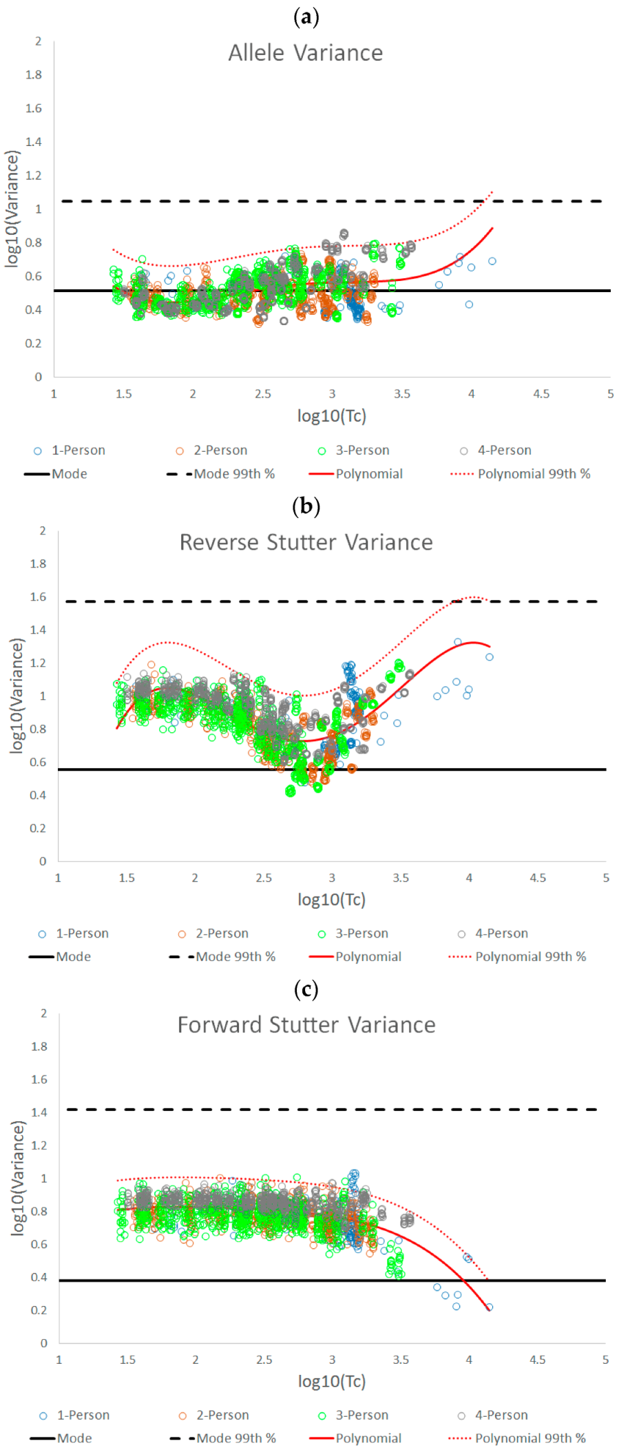
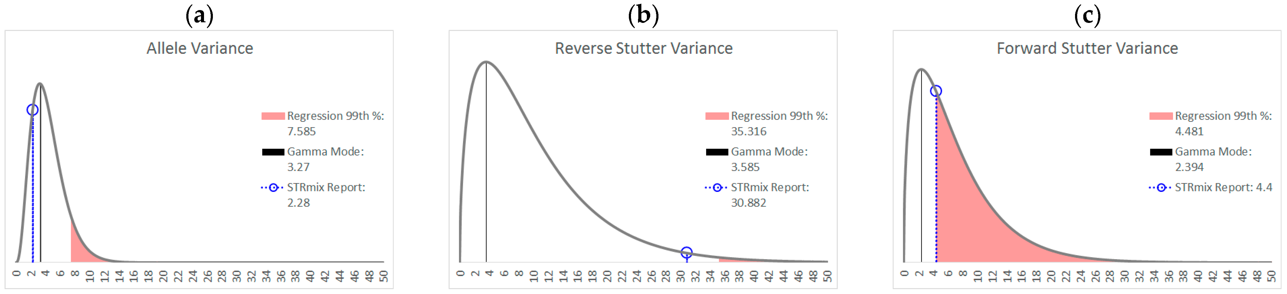
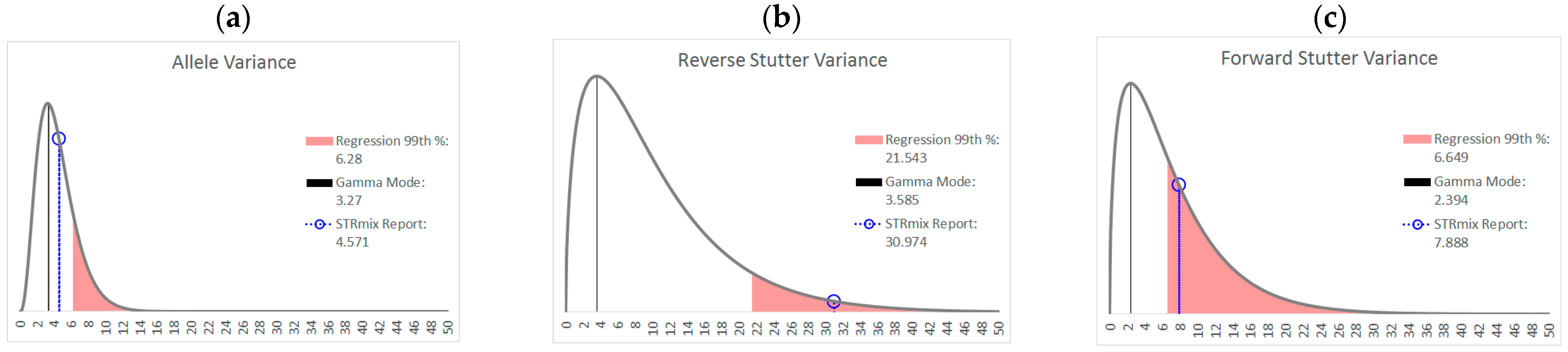
3.1. Trends in Allele and Stutter Variances with Increasing Peak Height
| Allele | Reverse Stutter | Forward Stutter | |
|---|---|---|---|
| Polynomial regression formula | y = 0.1122x4 − 1.2206x3 + 4.8535x2 − 8.2618x + 5.5312 | y = −0.2892x4 + 3.3258x3 − 13.619x2 + 23.456x − 13.404 | y = −0.0348x4 + 0.313x3 − 1.0891x2 + 1.7016x − 0.1678 |
| Jarque-Bera test for normality of the residuals | p = 0.1503 | p = 0.2395 | p = 0.0275 |
| 99th Percentile (+2.326 SD) | +0.2156 | +0.2755 | +0.1779 |
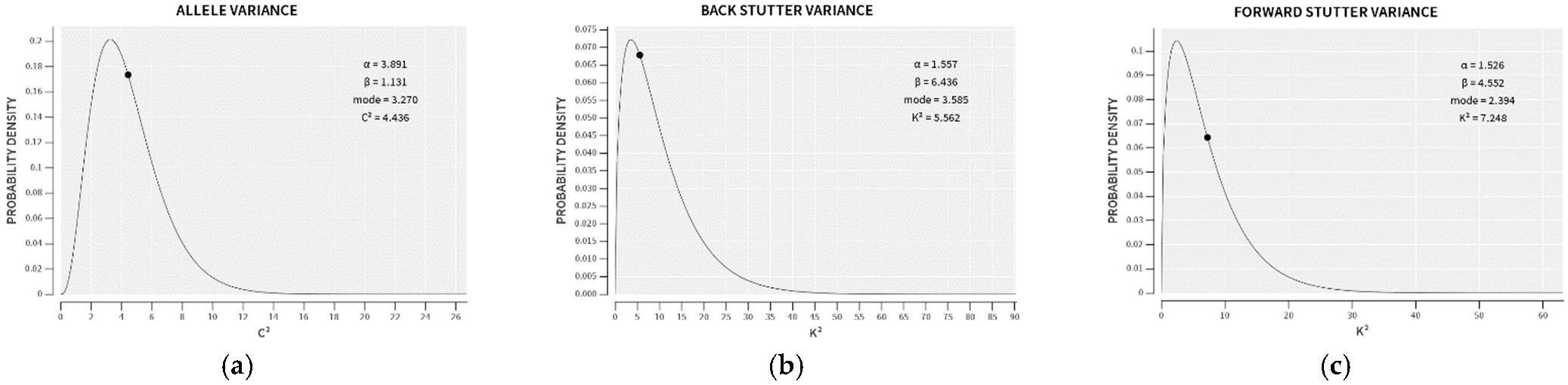
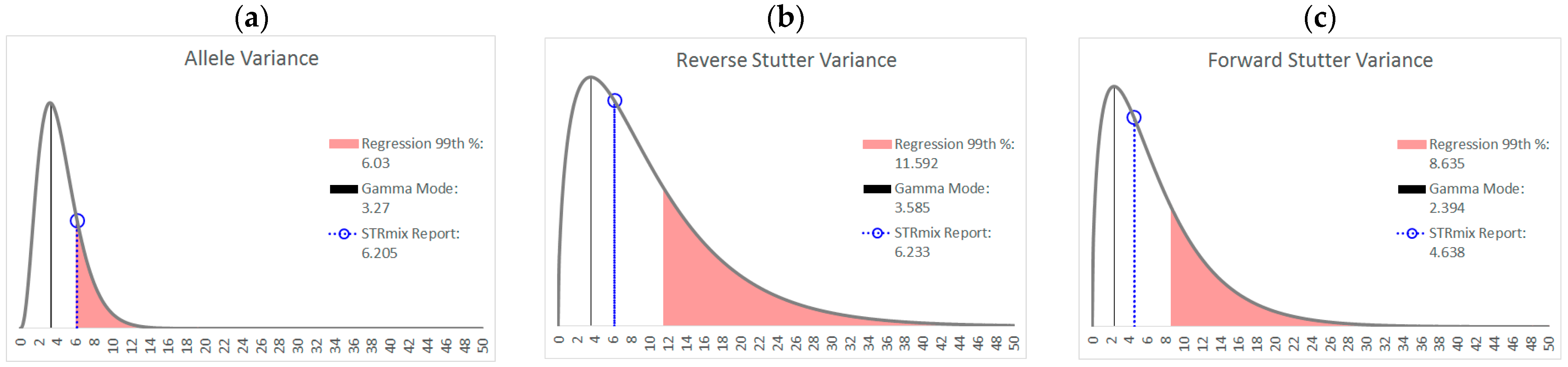
| Allele | Reverse Stutter | Forward Stutter | |
|---|---|---|---|
| α | 3.891 | 1.557 | 1.526 |
| β | 1.131 | 6.436 | 4.552 |
| Mode | 3.270 | 3.585 | 2.394 |
| 99th Percentile | 11.16 | 37.24 | 26.06 |
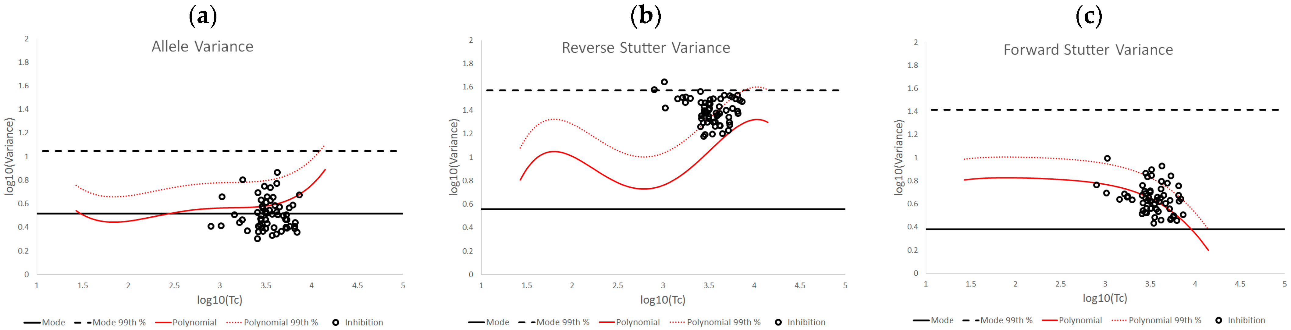
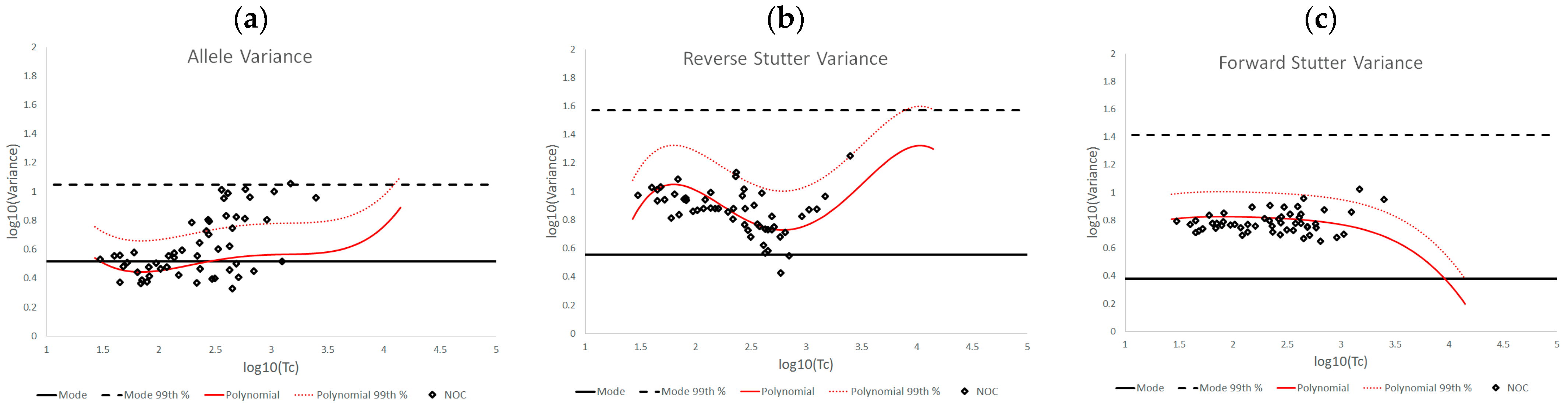
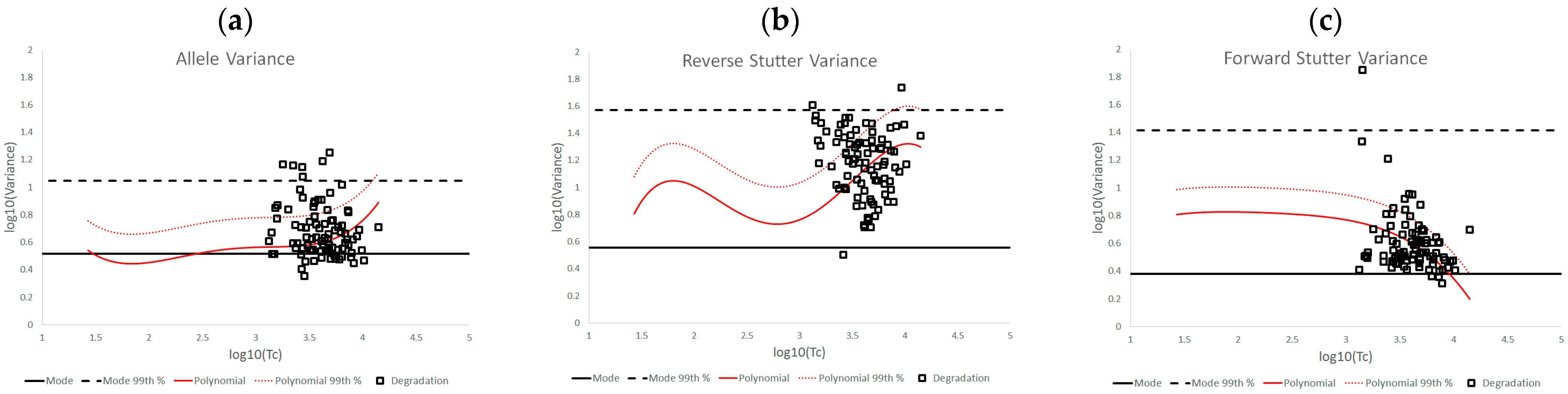
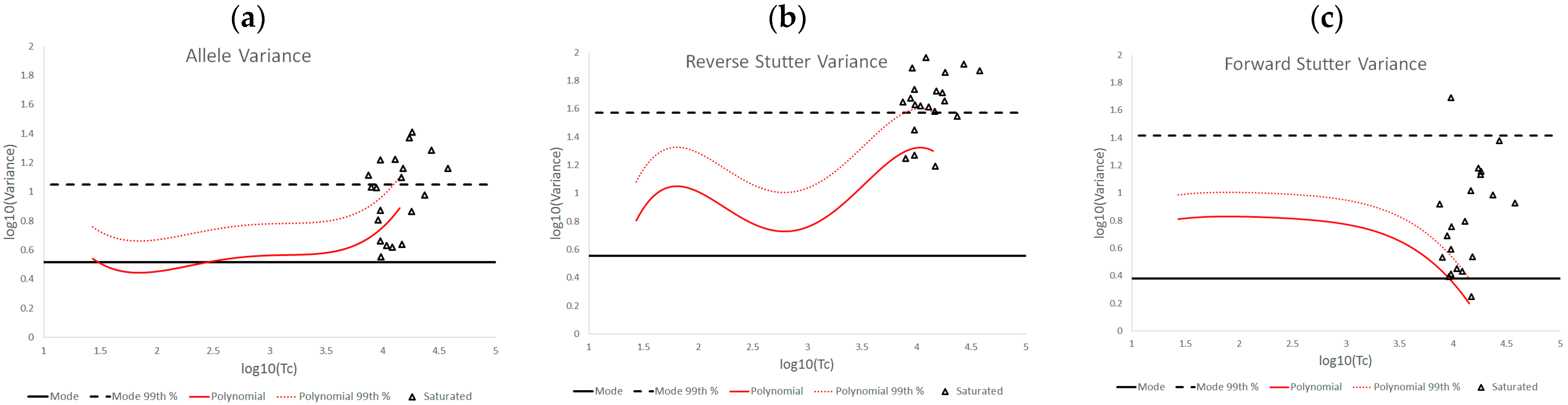
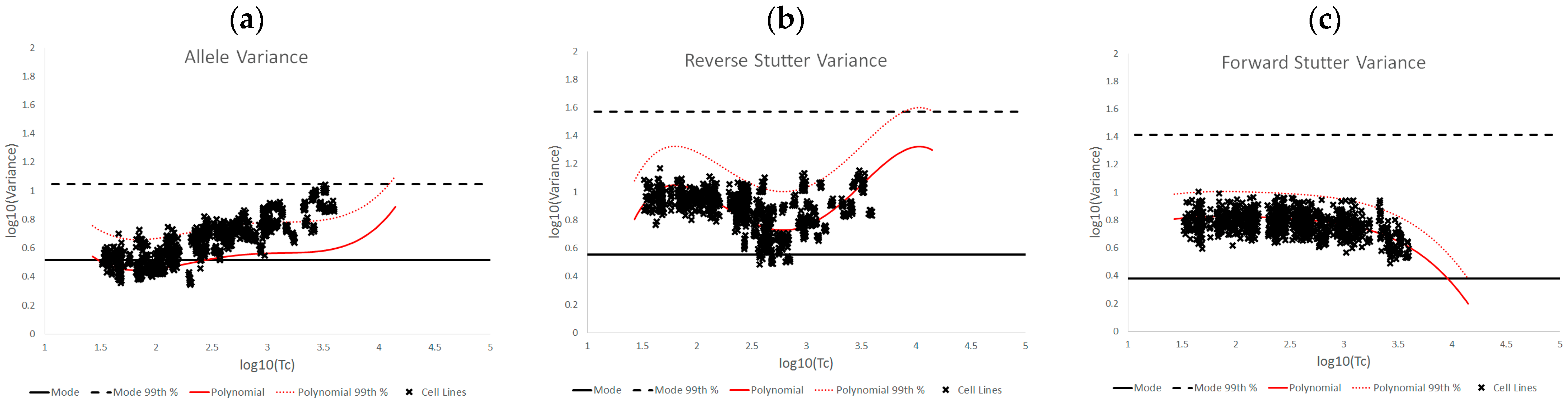
3.2. Trends in Allele and Stutter Variance under Challenging Amplification/Interpretation Conditions
4. Discussion
5. Conclusions
Supplementary Materials
Author Contributions
Funding
Informed Consent Statement
Data Availability Statement
Conflicts of Interest
References
- Clayton, T.M.; Whitaker, J.P.; Sparkes, R.; Gill, P. Analysis and interpretation of mixed forensic stains using DNA STR profiling. Forensic. Sci. Int. 1998, 91, 55–70. [Google Scholar] [CrossRef] [PubMed]
- Taylor, D.; Bright, J.A.; Buckleton, J. The interpretation of single source and mixed DNA profiles. Forensic. Sci. Int. Genet. 2013, 7, 516–528. [Google Scholar] [CrossRef] [PubMed]
- Taylor, D.; Buckleton, J.; Bright, J.A. Factors affecting peak height variability for short tandem repeat data. Forensic. Sci. Int. Genet. 2016, 21, 126–133. [Google Scholar] [CrossRef] [PubMed]
- Bille, T.W.; Weitz, S.M.; Coble, M.D.; Buckleton, J.; Bright, J.A. Comparison of the performance of different models for the interpretation of low level mixed DNA profiles. Electrophoresis 2014, 35, 3125–3133. [Google Scholar] [CrossRef] [PubMed]
- Bieber, F.R.; Buckleton, J.; Budowle, B.; Butler, J.M.; Coble, M.D. Evaluation of forensic DNA mixture evidence: Protocol for evaluation, interpretation, and statistical calculations using the combined probability of inclusion. BMC Genet. 2016, 17, 125. [Google Scholar] [CrossRef] [PubMed]
- Buckleton, J.; Bright, J.A.; Gittelson, S.; Moretti, T.; Onorato, A.J.; Bieber, F.R.; Budowle, B.; Taylor, D. The Probabilistic Genotyping Software STRmix: Utility and Evidence for its Validity. J. Forensic. Sci. 2019, 64, 393–405. [Google Scholar] [CrossRef] [PubMed]
- Bleka, Ø.; Storvik, G.; Gill, P. EuroForMix: An open source software based on a continuous model to evaluate STR DNA profiles from a mixture of contributors with artefacts. Forensic. Sci. Int. Genet. 2016, 21, 35–44. [Google Scholar] [CrossRef]
- Bright, J.A.; Taylor, D.; Curran, J.; Buckleton, J. Developing allelic and stutter peak height models for a continuous method of DNA interpretation. Forensic. Sci. Int. Genet. 2013, 7, 296–304. [Google Scholar] [CrossRef] [PubMed]
- STRmix v2.8 User’s Manual (September 2020); Institute of Environmental Science and Research Limited: Wellington, New Zealand, 2020.
- Russell, L.; Cooper, S.; Wivell, R.; Kerr, Z.; Taylor, D.; Buckleton, J.; Bright, J. A guide to results and diagnostics within a STRmix report. WIREs Forensic. Sci. 2019, 1, e1354. [Google Scholar] [CrossRef]
- Butler, J.M.; Iyer, H.; Press, R.; Taylor, M.K.; Vallone, P.M.; Willis, S. DNA Mixture INTERPRETATION: A NIST Scientific Foundation Review. NISTIR 8351-DRAFT; 2021. Available online: https://nvlpubs.nist.gov/nistpubs/ir/2021/NIST.IR.8351-draft.pdf (accessed on 17 November 2022).
- Duke, K.; Cuenca, D.; Myers, S.; Wallin, J. Compound and conditioned likelihood ratio behavior within a probabilistic genotyping context. Genes 2022, 13, 2031. [Google Scholar] [CrossRef] [PubMed]
- How to Perform a Normality Test in Excel (Step-by-Step). Available online: https://www.statology.org/normality-test-excel/ (accessed on 12 December 2022).
- Duke, K.; Myers, P. Systematic evaluation of STRmix™ performance on degraded DNA profile data. Forensic. Sci. Int. Genet. 2020, 44, 102174. [Google Scholar] [CrossRef] [PubMed]


| % Greater Than… | Unchallenged | Inhibited | NOC −1 or −2 | Degraded | Saturated | Cell Lines | |
|---|---|---|---|---|---|---|---|
| Allele Variance | Polynomial Regression | 48.90% | 21.67% | 67.92% | 53.33% | 55.00% | 90.50% |
| 99th Percentile | 1.05% | 3.33% | 28.30% | 21.11% | 40.00% | 21.84% | |
| Mode | 47.09% | 41.67% | 58.49% | 84.44% | 100.00% | 80.38% | |
| 99th Percentile | 0.00% | 0.00% | 1.89% | 6.67% | 45.00% | 0.00% | |
| Reverse Stutter Variance | Polynomial Regression | 50.91% | 100.00% | 39.62% | 57.78% | 85.00% | 45.60% |
| 99th Percentile | 1.15% | 56.67% | 3.77% | 23.33% | 80.00% | 1.92% | |
| Mode | 95.28% | 100.00% | 96.23% | 98.89% | 100.00% | 97.37% | |
| 99th Percentile | 0.00% | 3.33% | 0.00% | 2.22% | 75.00% | 0.00% | |
| Forward Stutter Variance | Polynomial Regression | 53.15% | 48.33% | 28.30% | 44.44% | 100.00% | 37.71% |
| 99th Percentile | 1.00% | 16.67% | 3.77% | 12.22% | 70.00% | 0.51% | |
| Mode | 99.76% | 100.00% | 100.00% | 96.67% | 95.00% | 100.00% | |
| 99th Percentile | 0.00% | 0.00% | 0.00% | 1.11% | 5.00% | 0.00% |
Disclaimer/Publisher’s Note: The statements, opinions and data contained in all publications are solely those of the individual author(s) and contributor(s) and not of MDPI and/or the editor(s). MDPI and/or the editor(s) disclaim responsibility for any injury to people or property resulting from any ideas, methods, instructions or products referred to in the content. |
© 2022 by the authors. Licensee MDPI, Basel, Switzerland. This article is an open access article distributed under the terms and conditions of the Creative Commons Attribution (CC BY) license (https://creativecommons.org/licenses/by/4.0/).
Share and Cite
Duke, K.; Myers, S.; Cuenca, D.; Wallin, J. Improving the Utilization of STRmix™ Variance Parameters as Semi-Quantitative Profile Modeling Metrics. Genes 2023, 14, 102. https://doi.org/10.3390/genes14010102
Duke K, Myers S, Cuenca D, Wallin J. Improving the Utilization of STRmix™ Variance Parameters as Semi-Quantitative Profile Modeling Metrics. Genes. 2023; 14(1):102. https://doi.org/10.3390/genes14010102
Chicago/Turabian StyleDuke, Kyle, Steven Myers, Daniela Cuenca, and Jeanette Wallin. 2023. "Improving the Utilization of STRmix™ Variance Parameters as Semi-Quantitative Profile Modeling Metrics" Genes 14, no. 1: 102. https://doi.org/10.3390/genes14010102
APA StyleDuke, K., Myers, S., Cuenca, D., & Wallin, J. (2023). Improving the Utilization of STRmix™ Variance Parameters as Semi-Quantitative Profile Modeling Metrics. Genes, 14(1), 102. https://doi.org/10.3390/genes14010102