A Framework for Evaluating Variation in (U-Th)/He Datasets


1
College of Earth, Ocean, and Atmospheric Sciences, Oregon State University, Corvallis, OR 97331, USA
2
Division of Geological and Planetary Sciences, California Institute of Technology, Pasadena, CA 91125, USA
*
Author to whom correspondence should be addressed.
Minerals 2020, 10(12), 1111; https://doi.org/10.3390/min10121111
Submission received: 11 November 2020
/
Revised: 6 December 2020
/
Accepted: 8 December 2020
/
Published: 10 December 2020
(This article belongs to the Section Mineral Geochemistry and Geochronology)
Abstract
:This paper presents a framework for evaluating variation in (U-Th)/He datasets. The framework is objective, repeatable, and based on compatibility of thermal histories derived from individual (U-Th)/He dates. The structure of this new method includes three fundamental steps. First, the allowable thermal history of each individual grain is quantitatively constrained with a model. Second, the thermal histories of all grains from a sample are visualized on the same axes. Third, the compatibility of the allowable thermal histories of each individual grain is evaluated. This allows a user to assess whether variation among single grain dates can plausibly be explained (referred to here as legitimate) or not (illegitimate). Additionally, this methodology allows for accurate representation of the impact that illegitimate variation has on the thermal history constraints of a sample. We demonstrate the application of this new framework using a variety of examples from the literature, as well as with synthetic data. Modeling presented here is executed using the modeling software QTQt (version 5.6.0) and the He diffusion kinetics based on the radiation damage accumulation and annealing model, but the framework is designed to be easily adaptable to any modeling software and diffusion parameters.
1. Introduction
(U-Th)/He dating of apatite is a broadly applied method in thermochronology [1,2,3]. The attraction of the method lies in the ubiquity of apatite in igneous, sedimentary, and metamorphic rocks and the method’s uniquely low closure temperature of 60–70 °C [1,4]. Although early applications of the method involved dating of multigrain aggregates (e.g., [4,5,6]), current standard practice is to date individual apatite crystals using a laser-heated microfurnace for He extraction (e.g., [7]). To test for internal repeatability, most investigators analyze between 4 and 10 crystals from a single rock (e.g., [8,9,10]) and frequently these individual dates do not agree within analytical uncertainty (e.g., [11,12,13]). In response, it has become common for investigators to apply some sort of data-filtering when interpreting a population of “overdispersed” (U-Th)/He dates [11,12]. Here we discuss why data filtering is ill-advised and offer an alternative approach to the interpretation of (U-Th)/He results on a population of single-grains from a given sample. Our method is applicable to rocks in which every grain must have experienced the same thermal history, and therefore excludes many sedimentary rocks. Although we focus on apatite, similar logic applies to zircon He dating [14,15].
Unlike dating of rock formation for example by U-Pb or K-Ar methods, the goal of thermochronometry is an acceptable set of time-temperature histories rather than a single geologically significant age. Here we emphasize this point by referring to (U-Th)/He dates (the result of a computation based on measured quantities) rather than ages (a geologically significant time in the past).
In a rock in which: (a) every analyzed grain experiences the same thermal history, and (b) every analyzed grain has the same diffusion kinetics, each grain should give the same cooling date. If both requirements hold, it makes sense to assess reproducibility among measured cooling dates and to identify and possibly reject outliers. However, as experience with the apatite (U-Th)/He system has grown, it has become increasingly apparent that criterion b is not valid. Instead, it is now known that grain size (e.g., [16,17]), accumulated radiation damage (e.g., [18,19,20]), and possibly apatite chemical composition (e.g., [21,22,23,24]) affect He diffusion kinetics and can therefore create a range of (U-Th)/He dates from a single rock. Under certain time-temperature conditions even tiny variations in diffusion parameters can create enormous variations in measured date. Each one of those dates can be completely valid and accurately reflect the causative time-temperature path. Consider the synthetic (U-Th)/He data shown in Table 1. As explained more fully in the table caption, these dates were all computed from a single time-temperature path on apatites that varied across a reasonable range of grain size and actinide concentrations. For present purposes the key point is that the span of dates, from 7.9 Ma to 91.7 Ma, or the mean and standard deviation 46.4 Ma +/- 34.5 Ma, both indicate variability far in excess of the typical analytical precision. This data set is apparently “overdispersed,” yet all dates are an accurate reflection of known phenomena.
Complicating matters, there are other phenomena that can yield (U-Th)/He dates that are not attributable to known variations in diffusivity of the associated grains. Examples of such phenomena are inaccurate analytical measurements, inaccurate alpha ejection corrections [25], the presence of mineral or fluid inclusions [1], alpha implantation from highly radioactive neighbors [26], and unrecognized zonation in U and Th [27]. More subtly, it is also likely that the small number of apatite specimens used to characterize He diffusion parameters (e.g., [17,18,21,28]) does not capture the true range among all natural apatite that is dated. In considering the latter it is important to recognize that He diffusion coefficients have almost invariably been measured on aggregates of hundreds of crystals analyzed simultaneously [4,29]. While such experiments capture the mean behavior, they inevitably miss real variability in diffusivity among individual apatites. Yet He dates are obtained on individual grains not on aggregates.
This leads to a conundrum. We know that some dispersion in measured dates from a single rock is fully expected, yet we also know that variability can result from phenomena that have not yet been, and perhaps cannot be, adequately documented, quantified, and represented in the numerical models used to interpret He dates in terms of causative cooling histories. Put simply, some analyzed apatite populations will have legitimate date variability, while others will have illegitimate date variability. Here legitimacy refers not to results of a statistical analysis of the dates themselves, but to whether existing models correctly capture the cause of the variability.
The goal of this paper is to provide a framework by which to distinguish legitimate from illegitimate variation. The proposed approach is to look for consistency not among the cooling dates, but among the cooling paths inverted from each grain analysis. Returning to the synthetic “overdispersed” data set, Figure 1 shows the result of individually inverting those dates for cooling paths. Each color represents the allowable thermal histories derived from the data of a different synthetic grain. This figure shows that all of the single grain dates can be explained by a single path; there is no illegitimate variability and any rejection of “date outliers” would weaken rather than strengthen the interpretation.
It is important to recognize that our understanding of legitimate vs illegitimate date variation has evolved rapidly over the last 20 years. In choosing examples that illustrate what we now recognize as inappropriate data filtering, we are not suggesting the original authors were careless or unscientific. Rather we are trying to clarify the current state-of-the-art and offer a path forward that takes advantage of our revised understanding of the (U-Th)/He system.
Published methods for dealing with potential outliers in (U-Th)/He datasets include a variety of approaches now recognized as problematic, such as
- removal of dates subjectively—this is enforced at the discretion of individual authors and is not necessarily explained. Rejected dates are sometimes attributed to the presence of inclusions, despite screening undertaken to eliminate grains with inclusions.
Examples presented later in this work will demonstrate how these methods are ill-advised given the current understanding of legitimate vs illegitimate variation. Because they are not based on a test of the compatibility of thermal histories, they can result in erroneous rejection of dates that appear to be “overdispersed” but actually vary legitimately. This poses the important problem: how to assess legitimacy of variation moving forward? The framework presented in this paper presents a solution to this question.
2. A Framework for Evaluating Variation
Two ideas form the foundation of the new framework for evaluating outliers in (U-Th)/He data presented here. The first is that a single (U-Th)/He date is consistent with a wide variety of potential thermal histories. The second is the concept that by minimizing external constraints, available modeling software allows for repeatable and objective, quantitative characterization of the range of allowable thermal histories for a single date. Based on this, we propose the following methodological framework for evaluating the legitimacy of variation (Figure 2).
- Run an independent model for each (U-Th)/He date.
- Visualize the model outputs for all single grains on a single set of time-temperature axes.
- If all data are compatible, then all variation is legitimate. Move forward with interpretation. Otherwise, illegitimate variation is present, and the sample should be flagged as such. Samples with illegitimate variation will contain less useful thermal history information than those with legitimate variation only. Rejecting a date is acceptable in the case that it is not geologically possible (e.g., if a date is older than a zircon U/Pb formation age of the same igneous sample).
Later sections will present new analysis of data from the literature that elucidate the application of this new framework through a series of examples that show the improvement of this over previously used methods. Before describing these examples, the next section describes the general modeling strategy.
3. Modeling Strategy
The two most widely used modeling programs in low-temperature thermochronology are QTQt and HeFTy [32,33]. Each utilizes a different statistical approach to constrain the thermal histories for a set of inputs. HeFTy randomly generates time-temperature paths and then calculates a goodness of fit parameter for each path, accepting only those which exceed a user-prescribed goodness of fit value. In some cases, no acceptable paths will be found. On the other hand, QTQt starts with an arbitrary thermal history and iteratively perturbs that history throughout a model run. After each iteration, a decision is made by the software to accept the better of the two according to an acceptance criterion. In doing this, QTQt always converges on a family of best posterior probability paths. After running QTQt for sufficient iterations such that the fit stops improving (referred to as the “burn in” period), the user then runs the program again for a set number of iterations, which fully explores the time-temperature space which characterizes the many thermal histories resultant in a roughly equivalent, allowable fit to the input data. The preferred visualization which we adopt for the results of this post “burn in” run is a plot of the population of accepted time-temperature paths from QTQt (e.g., Figure 3).
The statistical approaches taken by HeFTy and QTQt each have pros and cons (e.g., [34]), many of which have been discussed in the recent literature, including a set of comments and replies involving the authors of both software packages [35,36,37,38,39,40]. In the specific case where models are overconstrained by large or very scattered data sets, users of HeFTy will sometimes face a result of no acceptable time-temperature paths. But in such cases, QTQt will always yield a best-fit result, even if it does not match the input data. To avoid this pitfall, QTQt users must take care to document that their model results match the model inputs [13,35,38,41,42,43].
For the purposes of the application of QTQt in this work, the opposite of this overconstrained case is key—where one single input date is used with minimal external constraints. In such a case, the Bayesian approach employed by QTQt is highly effective at quantitatively constraining its allowable thermal histories. Because of this fact, we employ QTQt in all the model runs presented here.
The fundamental principle applied in setting up the QTQt model runs is that of minimal necessary constraint (MNC). The MNC principle requires that the only constraints placed on the model are (1) (U-Th)/He data and (2) direct constraints from geology or geochronology. Such observations might include a high temperature constraint from U-Pb data on a plutonic rock or a low temperature constraint from a known depositional age of a sedimentary unit. For the models presented later in this paper that evaluate published rejections, the only external constraints imposed on each model are the data from one single grain measurement and a modern-day low temperature constraint of 15 °C–20 °C. In the final example, a more tightly constrained sample is used. For all models, a required time-temperature bounding box is defined (15 °C–155 °C and 120 Ma–0 Ma). This bounding box serves as the prior for the inversion, and is used by QTQt primarily to assess whether to allow the birth or death of a node in the time-temperature path. Uncertainties are accounted for by employing the date resampling routine in QTQt.
It is worth noting that the algorithm employed by QTQt exhibits a preference for simplicity (e.g., a lower number of time-temperature points). This could affect the model results during the single grain model runs for samples that have particularly complex thermal histories. Also, a number of diffusion models are available to choose from in QTQt, including those of [28] and the RDAAM model of [18]. For the purposes of this paper, we employ the RDAAM model of [18]. These details are among the reasons that the methodological framework presented here for evaluating outliers is intentionally general, and is designed to be easily adaptable in the future for use with any choice of modeling software and diffusion kinetics (e.g., with HeFTy or the ADAM model of [44]).
4. A Synthetic Example
Before presenting new analysis of published data, we present details of the synthetic (U-Th)/He data mentioned above. This example shows how widely variable the legitimate dates could be from grains all taken from a sample with a single cooling history. For the example, a suite of synthetic (U-Th)/He data (six grains listed in Table 1) were input into HeFTy (version 1.9.3) where a forward model was used to determine their predicted dates for a common thermal history. All grains were forward modeled in HeFTy under a three-point thermal history starting at 15 °C at 100 Ma, heated monotonically to 75 °C at 10 Ma, and then cooled monotonically to 15 °C at 0 Ma (Figure 1). Utilizing the RDAAM He diffusion parameters [18], these six grains yield dates that increased with U, Th concentration and grain size, resulting in a wide range of dates. With the a priori knowledge that this variation is entirely legitimate, we treated these dates as a suite of data to evaluate using the newly proposed framework. First, an individual QTQt model run was set up for each grain. Next, the accepted post “burn in” thermal histories were plotted together (Figure 1A). Third, examining these paths reveals no incompatibility amongst individual grains, despite variation in date of over an order of magnitude (Table 1). As a result, the variation amongst these dates is judged to be legitimate. Finally, these six grains were input together into a QTQt model to demonstrate that QTQt could recover the original thermal history information from such a highly divergent suite of dates (Figure 1B).
5. Examining Published (U-Th)/He Data
Three data sources are presented here that are explored in detail later in this paper. The first two show different published examples where data was rejected [11,12], and the third presents a case where no data was rejected by its authors despite significant scatter [13]. All these data are evaluated using the new method outlined above. The data are shown in Table 2, where each date rejected by its authors is marked by an X.
5.1. Greater Caucasus
The first of these studies report apatite (U-Th)/He dates from ten rock samples from the Greater Caucasus [12]. We chose two of these ten—B2 and B5, as examples of outlier rejection for closer scrutiny. The analysis presented in [12] is one of many that utilizes a statistical standard that assumes a normally distributed population for rejecting outliers [10,12,47,48,49]. In this case, Dean’s Q-test [30] is applied to evaluate and reject one date per sample (Table 2, [12]). The Q-test is based on the calculation of a Q value according to Equation (1):
where is the potential outlier, is its nearest neighbor, and ω is the range. If Q exceeds a threshold value (tabulated in [30]), the datum can be rejected with 90% confidence. As is explained in [30], this is a useful heuristic for an outlier in a small sample from normally distributed population. As discussed above, based on our understanding of the (U-Th)/He system, there is no reason to expect a population of single grain dates from a rock to be normally distributed. Each grain is effectively a system with its own closure temperature, so there is no point to compute mean dates and consider normality of distributions.
5.2. Shillong Plateau (India)
The second published study is from the Shillong plateau in India [11]. Of a total of 13 samples with apatite (U-Th)/He data, one sample is chosen for further scrutiny, GP9S6 (Table 2; [11]). It is notable that [11] was published prior to widespread realization of legitimate grain to grain variation. Of the 6 grains reported for sample GP9S6, 4 were rejected without explanation. The only textual note in [11] about these rejections is in a Table footnote, which states that “Analyses were not taken in account when calculating the mean values.” (see Footnote b in Table 2 in [11]).
5.3. Western Sierra Nevada Foothills, California
The third study is from the western foothills of the southern Sierra Nevada in California [13]. Of a suite of 10 samples, the one with the largest number of single grains (11SS6, n = 7) is chosen for further scrutiny. The seven apatite (U-Th)/He single grain dates range from 81.2 to 112.6 Ma (Table 2), and none of the dates were rejected by [13]. This is a good trial sample to assess the newly proposed standard for evaluating variation due to the large number of dates and the significant variation displayed amongst the dates (the range, 31.4 m.y., is 36% of the median date, 86.9 Ma). The sampled pluton is dated at circa 114 Ma [50]. At the sample location, the pluton is nonconformably overlain by Eocene Ione Formation [13]. This provides significant time-temperature control on the bedrock sampled. These external constraints were input into the thermal model as a high temperature constraint (550–750 °C at 109–119 Ma) and a low temperature constraint (15–20 °C at 35–45 Ma).
6. Evaluating Variation
6.1. Step One: Single Grain Model Runs
The first step in evaluating variation is to set up and run a model for each individual dated grain. This requires building a single data file for each grain, inputting the constraints into the QTQt interface, and running the model. For B2, B5 and GP9S6, external constraints are limited to a modern low temperature surface constraint according to the MNC principle. For 11SS6, both a high temperature and low temperature constraint were input. All models are run for at least 500,000 “burn in” iterations and 500,000 post “burn in” iterations, after [13,35,41,43].
6.2. Step Two: Visualize Single Grain Model Results
The next step in evaluating whether variation is legitimate is to visualize the results of the post “burn in” single grain model runs by plotting the accepted time-temperature paths (e.g., Figure 3).
6.3. Step Three: Evaluate Legitimacy of Variation Based on Compatibility of Thermal Histories
After plotting the single grain model results together, the critical task remains to use this visualization to determine whether illegitimate variation is present. If any of the dates yield model results that are incompatible with other dates, then illegitimate variation is present within the sample. If all variation is legitimate (e.g., Figure 3), no further scrutiny is required, and the user can continue with interpretation of the sample thermal history.
6.3.1. Erroneous Rejection of Legitimate Data
The example shown in Figure 3 represents a rejection from Sample B5 [12] of a date that varied legitimately. The blue lines (Figure 3) represent the allowable thermal histories for grains that were not rejected, and the red lines represent the results for the rejected date. The rejected grain, B5-1, was tested with a Q-value and rejected by [12]. However, when the acceptable thermal histories of all individual grains are visualized together, there is no incompatibility between grain B5-1 and the grouping of younger grains (B5-2, B5-3, and B5-4). This is most clearly shown by the presence of some accepted red paths centrally within the overlapping blue zone (white arrow on Figure 3). The reason why the model is able to find paths that fit B5-1 (53 Ma) and B5-2/3/4 (15 Ma, 21 Ma, 21 Ma) is that the older grain is significantly larger (118 μm) than the three younger grains (45 μm, 52 μm, 53 μm). In this case, the grain size effect on closure temperature explains most of the variation amongst measured dates (Figure 4). Because all variation is legitimate in this sample, the investigator should move straight to interpretating the sample thermal history without rejecting any data.
6.3.2. Rejection of Illegitimate Data
In contrast to the first example, Figure 5 shows an example of a rejected date from a sample that displays some illegitimate variation (sample B2). In the initial study, a Q-test was used to reject B2-3 as an outlier [12]. Under step three of the new framework, sample B2 would be flagged as containing illegitimate variation. The thermal history of grain B2-3 (shown in red on Figure 5A) is different from that of the other four grains.
One way to approach this illegitimate variation would be to assert that the thermal history shown in red should be rejected. However, each of the individual dates is equally valid from an analytical standpoint. It may be tempting to choose on the basis of the number of analyses per grouping, but there is nothing inherent in the data that indicates whether B2-3 is illegitimate or whether B2-1, B2-2, B2-4, and B2-5 are illegitimate. For example, if all four of the younger grains (B2-1/2/4/5) are strongly zoned with a high U rim and low U core, but B2-3 has a homogeneous U concentration, the grouping of four young grains would be illegitimate, and the older grain would be correct. Because the data do not allow for positive identification of which dates are illegitimate, rejecting any individual dates is ill-advised.
Another tempting way to consider interpreting the thermal history of this sample is to input all the grains from the illegitimate sample into a QTQt model run. The results of this are shown in green on Figure 5B. As these results show, QTQt allows for a wide range of possible thermal histories, which partially agrees with the thermal histories of each single grain within the last ~4 m.y.. However, during the timespan of circa 4 Ma to 7 Ma, the model result heavily favors the thermal histories that fit B2-1, B2-2, B2-4, and B2-5 over those that fit B2-3. For this part of the thermal history, this result is effectively rejecting all but the most numerous grouping of data. As we have already discussed, the data do not allow for a positive determination that B2-3 is illegitimate. Because of this, inputting all the single grain data into QTQt is ill-advised. When the variation amongst dates is illegitimate, QTQt cannot honor the thermal history constraints of all the inputs, and so asking it to sort out the illegitimate variation can lead to flawed interpretation.
To avoid these potentially incorrect results, our preferred approach to interpreting the thermal history of a sample with more than one distinct grouping of thermal histories is to: (1) not reject any data and (2) recognize that it contains little definitive thermal history information. The most meaningful visualization of the thermal history information of this sample is the plot of the single grain model results together (Figure 5A). Based on the geologic context of the sample, a user may be able to determine that a subset of the allowable thermal histories is preferred, but no discrimination beyond this can be gleaned from the data alone.
6.4. Additional Examples
The examples presented above were chosen to explicitly demonstrate the key characteristics of the new framework for evaluating variation, and to show how previous methods fall short. Experienced workers will readily anticipate many possible suites of (U-Th)/He data that are more difficult to assess than those presented in the examples above. While it is not realistic to exhaustively evaluate all possible cases, it is worth discussing a few more scenarios. These examples are meant to clarify the intent of the standard proposed in this work: to establish a useful method of assessing the legitimacy of variation that is based on compatibility amongst acceptable thermal histories.
6.4.1. Disparate Dates
The first scenario is that of disparate data that are characterized by widely varying dates. Such a case is exemplified by sample GP9S6 [11]. In this case, four dates were rejected from a population of 6, leaving only 2 accepted dates (Figure 6). Visual comparison of the model results of all six individual grains show inconsistency between GP9S6-1 and grains GP9S3/6. Furthermore, GP9S6-2, GP9S6-4, and GP9S6-5 closely overlap with each other and completely fill the gap between GP9S6-1 and GP9S6-3/6.
Applying the newly proposed framework, the sample should be flagged for containing illegitimate variation. Stated differently, the variation in dates observed in this sample has no presently known cause. The thermal history of GP9S6-1 is incompatible with that of GP9S6-3 and 6. This case exhibits three distinct groupings with intra-group consistency but inter-group inconsistency. Because there is no reason to prefer any one of these groupings over another, our preferred approach would be to keep all data but flag the variation as illegitimate.
One tempting way to approach interpreting this sample would be to input all the data together into a QTQt model run (green lines on Figure 6B). However, the QTQt result is not compatible with all of the input data. Specifically, the preferred QTQt result is inconsistent with all the allowable thermal histories of GP9S6-1 for the period between roughly 15 Ma and 20 Ma. The illegitimacy of variation in this sample is the cause of this inconsistency. QTQt cannot find a thermal history that accommodates all of the input data because no such thermal history exists. In this case, as in the previous example of illegitimate variation, inputting all the data into a single QTQt model is ill-advised.
Rather, our preferred approach to interpreting the thermal history of a sample with a broad spectrum of internally consistent but externally inconsistent groupings is to: (1) not reject any data and (2) recognize that it contains limited useful thermal history information. The most meaningful visualization of the thermal history information of this sample is a plot of the single grain model results together (Figure 6A). Based on the geologic context of the sample, a user may be able to determine that a subset of the allowable thermal histories is preferred, but no discrimination beyond this can be gleaned from the He alone.
The examples discussed above focus on reassessing published rejections of individual dates. In the next section an additional example from the literature will be considered in which the authors did not reject any dates, despite significant variation.
6.4.2. Legitimate Variation
The results of individual grain models from sample 11SS6 show no incompatibility amongst allowable thermal histories despite significant date variation (Figure 7). As a result, all variation present in this sample is legitimate, and the investigator should continue with interpretation of the sample thermal history. This confirms the decision taken to accept all data [13]. Despite the large range in measured single grain dates, there is overlap in the allowable thermal histories of all the individual grain dates, even between the youngest and oldest grains (blue and red, respectively in Figure 7).
7. Discussion
The framework presented above for evaluating variation in (U-Th)/He datasets provides an objective and repeatable method that is based on the use of a modeling approach to quantitatively constrain the allowable time-temperature histories of individual dates. This is a major advance over published methods of removing outliers that rely on an assumed normal distribution. The application of a Q-test from [12] results in rejection of dates without determining illegitimacy. The underlying assumption of a normally distributed population is not appropriate, and the Q-test is an unreliable and unacceptable test for (U-Th)/He data.
7.1. Modeling Strategy
As described above, for the purposes of the examples given in this paper, the modeling software QTQt was employed and apatite diffusion kinetics were set according to the RDAAM model of [18]. The modeling of single grains requires a choice of specific tools, and the implementation used in this paper is specifically designed to leverage the strengths of QTQt to quantitatively constrain the allowable thermal histories of individual dates in an objective and repeatable way by applying the MNC principle. However, it is important to note that the framework for evaluating variation is general, and purposely not dependent on the tools applied here. For example, one could use HeFTy instead of QTQt to model the allowable thermal histories of single grain dates, and one could choose to use a different model for the effect of radiation damage on apatite diffusion kinetics. In the future, if new and better software and diffusion models become available, this framework for evaluating outliers will be readily adaptable.
7.2. Interpreting Dates
The concept of legitimate versus illegitimate variation provides a scaffolding for determining when “overdispersion” in (U-Th)/He datasets is usefully interpretable (legitimate) and when it is not (illegitimate). When variation is legitimate, so-called “overdispersion” is just a result of varying diffusion kinetics within the scope of currently understood parameters (e.g., sample B5 or the synthetic example provided earlier). When varying diffusion kinetics cannot explain the range of dates, illegitimate variation is present.
The methodological framework presented here is designed to evaluate the legitimacy of variation in (U-Th)/He data at the very beginning of the interpretation phase of the scientific workflow, and prior to the geologic interpretation of a sample’s thermal history. Because the legitimacy of variation amongst individual dates has important implications on the final interpretation of any suite of data, examples of interpretive methods are sometimes presented alongside the assessment of legitimacy in this paper.
The examples presented here highlight the fact that when illegitimate variation is present within a sample, inputting all the data into QTQt is ill-advised. Because no thermal history can explain the illegitimate data variation, the model result will not honor all the input data. Furthermore, with our current understanding of apatite (U-Th)/He systematics, we have no reliable method of deciding which inputs should be rejected, and which should be accepted. Therefore, our preferred approach to interpreting the thermal history of such a sample is to: (1) not reject any data but flag the sample as illegitimate and (2) accept the fact that the data contains limited thermal history information. This problem is not soluble by thermal history modeling.
Moreover, it is critical that the determination of whether variation is legitimate occurs prior to, and separate from, the geologic interpretation of a sample’s thermal history. While a similar methodology of graphical overlay of acceptable single grain thermal histories has been published recently (e.g., [42]), the most common methods for modeling (U-Th)/He data involve simultaneous constraint by more than one individual grain date. This can be applied in a wide variety of contexts, such as constraining timing and rate of exhumation, simultaneous modeling of entire vertical transects, constraining the timing of activity on individual structures, and considering (U-Th)/He data from multiple mineral phases or other thermochronometric systems (e.g., [13,43,51,52,53,54,55,56,57,58]). While different applications may require specific approaches to the interpretation of dates, the method proposed here is universally applicable in cases where workers are considering potentially illegitimate variation in (U-Th)/He datasets.
The framework for assessing outliers in (U-Th)/He data presented here is only applicable in cases where all of the grains from a sample have a shared thermal history in the temperature range of the apatite He partial retention zone, generally less than 100 °C. Because this shared history is necessary for the new methodological framework introduced here to be useful, it is not applicable to any detrital samples that are not reset post-depositionally.
8. Conclusions
(U-Th)/He data inform our understanding of a wide range of geologic and Earth surface processes. The ongoing evolution in our understanding of the factors controlling He diffusion in minerals and computational tools for extracting thermal history information from data continues to widen the scope of applications of low temperature thermochronometric data. Despite this breadth of applications, until now published methods for deciding how to handle potentially illegitimate data have been unreliable, subjective, and rooted in assumptions that are fundamentally flawed. Because diffusion kinetics can vary widely in nature, seemingly “overdispersed” dates can be fully compatible with a single thermal history (they are legitimate). This demands an objective and repeatable methodology for evaluating the legitimacy of variation that is rooted in the fundamental information recorded by the data – the thermal histories of the analyzed grains. This paper presents a framework that fulfills these requirements, highlights examples of its application to data previously interpreted differently and lays out a method that is easily adaptable by future workers to new modeling approaches and new diffusion parameters. The method is outlined as follows.
- Model each individual grain independently. Employ the principle of minimum necessary constraint (MNC).
- Visualize the acceptable thermal histories of each grain together on a single set of time-temperature axes.
- Decide whether variation amongst individual dates is legitimate by considering the compatibility amongst allowable thermal histories of each date. Flag illegitimate samples.
Author Contributions
Conceptualization, F.J.S. and K.A.F.; Data curation, F.J.S.; Funding acquisition, F.J.S; Investigation, F.J.S.; Methodology, F.J.S.; Writing—original draft, F.J.S; Writing—review & editing, F.J.S. and K.A.F. All authors have read and agreed to the published version of the manuscript.
Funding
This research received no external funding.
Acknowledgments
The Oregon State University Geomorphology Round Table is gratefully acknowledged for providing feedback on the intellectual framework of this project at an early stage. Lindsey Hedges is gratefully thanked for a lifetime of service to geochemistry.
Conflicts of Interest
The authors declare no conflict of interest.
References
- Gallagher, K. Transdimensional inverse thermal history modeling for quantitative thermochronology. J. Geophys. Res. Solid Earth 2012, 117, B02408. [Google Scholar] [CrossRef] [Green Version]
- Flowers, R.M.; Ketcham, R.A.; Shuster, D.L.; Farley, K.A. Apatite (U–Th)/He thermochronometry using a radiation damage accumulation and annealing model. Geochim. Cosmochim. Acta 2009, 73, 2347–2365. [Google Scholar] [CrossRef]
- Farley, K.A. (U-Th)/He dating: Techniques, calibrations, and applications. Rev. Mineral. Geochem. 2002, 47, 819–844. [Google Scholar] [CrossRef]
- Ehlers, T.A.; Farley, K.A. Apatite (U–Th)/He thermochronometry: Methods and applications to problems in tectonic and surface processes. Earth Planet. Sci. Lett. 2003, 206, 1–14. [Google Scholar] [CrossRef]
- Reiners, P.W.; Ehlers, T.A.; Zeitler, P.K. Past, present, and future of thermochronology. Rev. Mineral. Geochem. 2005, 58, 1–18. [Google Scholar] [CrossRef] [Green Version]
- Wolf, R.A.; Farley, K.A.; Silver, L.T. Helium diffusion and low temperature thermochronometry of apatite. Geochim. Cosmochim. Acta 1996, 60, 4231–4240. [Google Scholar] [CrossRef]
- House, M.A.; Wernicke, B.P.; Farley, K.A.; Dumitru, T.A. Cenozoic thermal evolution of the central Sierra Nevada, California, from (UTh)/He thermochronometry. Earth Planet. Sci. Lett. 1997, 151, 167–179. [Google Scholar] [CrossRef]
- Zeitler, P.K.; Herczeg, A.L.; McDougall, I.; Honda, M. U-Th-He dating of apatite: A potential thermochronometer. Geochim. Cosmochim. Acta 1987, 51, 2865–2868. [Google Scholar] [CrossRef]
- House, M.A.; Farley, K.A.; Stockli, D. Helium chronometry of apatite and titanite using Nd-YAG laser heating. Earth Planet. Sci. Lett. 2000, 183, 365–368. [Google Scholar] [CrossRef]
- Reiners, P.W.; Ehlers, T.A.; Garveer, J.I.; Mitchell, S.G.; Montgomery, D.R.; Vance, J.A.; Nicolescu, S. Late Miocene exhumation and uplift of the Washington Cascade Range. Geology 2002, 30, 767–770. [Google Scholar] [CrossRef] [Green Version]
- Stockli, D.F.; Dumitru, T.A.; McWilliams, M.O.; Farley, K.A. Cenozoic tectonic evolution of the White Mountains, California and Nevada. Geol. Soc. Am. Bull. 2003, 115, 788–816. [Google Scholar] [CrossRef]
- Staisch, L.M.; Niemi, N.A.; Clark, M.K.; Chang, H. Eocene to late Oligocene history of crustal shortening within the Hoh Xil Basin and implications for the uplift history of the northern Tibetan Plateau. Tectonics 2016, 35, 862–895. [Google Scholar] [CrossRef] [Green Version]
- Biswas, S.; Coutand, I.; Grujic, D.; Hager, C.; Stockli, D.; Grasemann, B. Exhumation and uplift of the Shillong plateau and its influence on the eastern Himalayas: New constraints from apatite and zircon (U-Th-[Sm])/He and apatite fission track analyses. Tectonics 2007, 26, TC6013. [Google Scholar] [CrossRef]
- Avdeev, B.; Niemi, N.A. Rapid Pliocene exhumation of the central Greater Caucasus constrained by low-temperature thermochronometry. Tectonics 2011, 30, TC2009. [Google Scholar] [CrossRef] [Green Version]
- Sousa, F.J.; Saleeby, J.; Farley, K.A.; Unruh, J.R.; Lloyd, M.K. The southern Sierra Nevada pediment, central California. Geosphere 2017, 13, 82–101. [Google Scholar] [CrossRef]
- Reiners, P.W.; Farley, K.A.; Hickes, H.J. He diffusion and (U–Th)/He thermochronometry of zircon: Initial results from Fish Canyon Tuff and Gold Butte. Tectonophysics 2002, 349, 297–308. [Google Scholar] [CrossRef]
- Reiners, P.W.; Spell, T.L.; Nicolescu, S.; Zanetti, K.A. Zircon (U-Th)/He thermochronometry: He diffusion and comparisons with 40Ar/39Ar dating. Geochim. Cosmochim. Acta 2004, 68, 1857–1887. [Google Scholar] [CrossRef]
- Dodson, M.H. Closure temperature in cooling geochronological and petrological systems. Contrib. Mineral. Petrol. 1973, 40, 259–274. [Google Scholar] [CrossRef]
- Farley, K.A. Helium diffusion from apatite: General behaviors as illustrated by Durango fluorapatite. J. Geophys. Res. 2000, 105, 2903–2914. [Google Scholar] [CrossRef] [Green Version]
- Gerin, C.; Gautheron, C.; Oliviero, E.; Bachelet, C.; Djimbi, D.M.; Seydoux-Guillaume, A.M.; Tassan-Got, L.; Sarda, P.; Roques, J.; Garrido, F. Influence of vacancy damage on He diffusion in apatite, investigated at atomic to mineralogical scales. Geochim. Cosmochim. Acta 2017, 197, 87–103. [Google Scholar] [CrossRef]
- Flowers, R.M.; Kelley, S.A. Interpreting data dispersion and “inverted” dates in apatite (U–Th)/He and fission-track datasets: An example from the US midcontinent. Geochim. Cosmochim. Acta 2011, 75, 5169–5186. [Google Scholar] [CrossRef]
- Shuster, D.L.; Flowers, R.M.; Farley, K.A. The influence of natural radiation damage on helium diffusion kinetics in apatite. Earth Planet. Sci. Lett. 2006, 249, 148–161. [Google Scholar] [CrossRef]
- Warnock, A.C.; Zeitler, P.K.; Wolf, R.A.; Bergman, S.C. An evaluation of low-temperature apatite U Th/He thermochronometry. Geochim. Cosmochim. Acta 1997, 61, 5371–5377. [Google Scholar] [CrossRef]
- Recanati, A.; Gautheron, C.; Barbarand, J.; Missenard, Y.; Pinna-Jamme, R.; Tassan-Got, L.; Carter, A.; Douville, E.; Bordier, L.; Pagel, M.; et al. Helium trapping in apatite damage: Insights from (U-Th-Sm)/He dating of different granitoid lithologies. Chem. Geol. 2017, 470, 116–131. [Google Scholar] [CrossRef] [Green Version]
- McDannell, K.T.; Zeitler, P.K.; Janes, D.G.; Idleman, B.D.; Fayon, A.K. Screening apatites for (U-Th)/He thermochronometry via continuous ramped heating: He age components and implications for age dispersion. Geochim. Cosmochim. Acta 2018, 223, 90–106. [Google Scholar] [CrossRef]
- Cooperdock, E.H.G.; Ketcham, R.A.; Stockli, D.F. Resolving the effects of 2-D versus 3-D grain measurements on apatite (U–Th)/He age data and reproducibility. Geochronology 2019, 1, 17–41. [Google Scholar] [CrossRef] [Green Version]
- Gautheron, C.; Tassan-Got, L.; Ketcham, R.A.; Dobson, K.J. Accounting for long alpha-particle stopping distances in (U–Th–Sm)/He geochronology: 3D modeling of diffusion, zoning, implantation, and abrasion. Geochim. Cosmochim. Acta 2012, 96, 44–56. [Google Scholar] [CrossRef] [Green Version]
- Farley, K.A.; Shuster, D.L.; Ketcham, R.A. U and Th zonation in apatite observed by laser ablation ICPMS, and implications for the (U–Th)/He system. Geochim. Cosmochim. Acta 2011, 75, 4515–4530. [Google Scholar] [CrossRef]
- Gautheron, C.; Tassan-Got, L.; Barbarand, J.; Pagel, M. Effect of alpha-damage annealing on apatite (U–Th)/He thermochronology. Chem. Geol. 2009, 266, 157–170. [Google Scholar] [CrossRef]
- Wolf, R.A.; Farley, K.A.; Silver, L.T. Assessment of (U-Th)/He thermochronometry: The low-temperature history of the San Jacinto mountains, California. Geology 1997, 25, 65–68. [Google Scholar] [CrossRef]
- Dean, R.B.; Dixon, W.J. Simplified Statistics for Small Numbers of Observations. Anal. Chem. 1951, 23, 636–638. [Google Scholar] [CrossRef]
- Boddy, R.; Smith, G. Effective Experimentation: For Scientists and Technologists; John Wiley & Sons: Hoboken, NJ, USA, 2011. [Google Scholar]
- Ketcham, R.A. Forward and inverse modeling of low-temperature thermochronometry data. Rev. Mineral. Geochem. 2005, 58, 275–314. [Google Scholar] [CrossRef]
- Fox, M.; Carter, A. Heated Topics in Thermochronology and Paths towards Resolution. Geosciences 2020, 10, 375. [Google Scholar] [CrossRef]
- Vermeesch, P.; Tian, Y. Thermal history modelling: HeFTy vs. QTQt. Earth Sci. Rev. 2014, 139, 279–290. [Google Scholar] [CrossRef] [Green Version]
- Vermeesch, P.; Tian, Y. Reply to Comment on “Thermal history modelling: HeFTy vs. QTQt” by K. Gallagher and R.A. Ketcham. Earth Sci. Rev. 2018, 176, 395–396. [Google Scholar] [CrossRef]
- Gallagher, K.; Ketcham, R.A. Comment on “Thermal history modelling: HeFTy vs. QTQt” by Vermeesch and Tian, Earth-Science Reviews (2014), 139, 279–290. Earth Sci. Rev. 2018, 176, 387–394. [Google Scholar] [CrossRef]
- Gallagher, K. Comment on ‘A reporting protocol for thermochronologic modeling illustrated with data from the Grand Canyon’ by Flowers, Farley and Ketcham. Earth Planet. Sci. Lett. 2016, 441, 211–212. [Google Scholar] [CrossRef]
- Flowers, R.M.; Farley, K.A.; Ketcham, R.A. A reporting protocol for thermochronologic modeling illustrated with data from the Grand Canyon. Earth Planet. Sci. Lett. 2015, 432, 425–435. [Google Scholar] [CrossRef] [Green Version]
- Flowers, R.M.; Farley, K.A.; Ketcham, R.A. Response to comment on “A reporting protocol for thermochronologic modeling illustrated with data from the Grand Canyon”. Earth Planet. Sci. Lett. 2016, 441, 213. [Google Scholar] [CrossRef]
- Sousa, F.J. Eocene Origin of Owens Valley, California. Geosciences 2019, 9, 194. [Google Scholar] [CrossRef] [Green Version]
- Gavillot, Y.; Meigs, A.J.; Sousa, F.J.; Stockli, D.; Yule, D.; Malik, M. Late Cenozoic Foreland-to-Hinterland Low-Temperature Exhumation History of the Kashmir Himalaya. Tectonics 2018, 37, 3041–3068. [Google Scholar] [CrossRef]
- Sousa, F.J.; Farley, K.A.; Saleeby, J.; Clark, M. Eocene activity on the Western Sierra Fault System and its role incising Kings Canyon, California. Earth Planet. Sci. Lett. 2016, 439, 29–38. [Google Scholar] [CrossRef] [Green Version]
- Willett, C.D.; Fox, M.; Shuster, D.L. A helium-based model for the effects of radiation damage annealing on helium diffusion kinetics in apatite. Earth Planet. Sci. Lett. 2017, 477, 195–204. [Google Scholar] [CrossRef] [Green Version]
- Ketcham, R.A.; Gautheron, C.; Tassan-Got, L. Accounting for long alpha-particle stopping distances in (U–Th–Sm)/He geochronology: Refinement of the baseline case. Geochim. Cosmochim. Acta 2011, 75, 7779–7791. [Google Scholar] [CrossRef]
- Gautheron, C.; Tassan-Got, L. A Monte Carlo approach to diffusion applied to noble gas/helium thermochronology. Chem. Geol. 2010, 273, 212–224. [Google Scholar] [CrossRef]
- Lossada, A.C.; Giambiagi, L.; Hoke, G.D.; Fitzgerald, P.G.; Creixell, C.; Murillo, I.; Mardonez, D.; Velásquez, R.; Suriano, J. Thermochronologic Evidence for Late Eocene Andean Mountain Building at 30° S. Tectonics 2017, 36, 2693–2713. [Google Scholar] [CrossRef]
- Abbey, A.L.; Niemi, N.A.; Geissman, J.W.; Winkelstern, I.Z.; Heizler, M. Early Cenozoic exhumation and paleotopography in the Arkansas River valley, southern Rocky Mountains, Colorado. Lithosphere 2017, 10, 239–266. [Google Scholar] [CrossRef] [Green Version]
- Abbey, A.L.; Niemi, N.A. Low-temperature thermochronometric constraints on fault initiation and growth in the northern Rio Grande rift, upper Arkansas River valley, Colorado, USA. Geology 2018, 46, 627–630. [Google Scholar] [CrossRef]
- Bateman, P.C.; Busacca, A.J.; Sawka, W.N. Cretaceous Deformation in the Western Foothills of the Sierra-Nevada, California. Geol. Soc. Am. Bull. 1983, 94, 30–42. [Google Scholar] [CrossRef]
- Saleeby, J.; Saleeby, Z.; Sousa, F. From deep to modern time along the western Sierra Nevada Foothills of California, San Joaquin to Kern River drainages. Geol. Soc. Am. Field Guides 2013, 32, 37–62. [Google Scholar] [CrossRef]
- Sousa, F.; Saleeby, J.; Farley, K.A.; Unruh, J. The Southern Sierra Nevada Foothills Bedrock Pediment. In Proceedings of the 2013 GSA Cordilleran Section Meeting, Fresno, CA, USA, 20–22 May 2013; p. 53. [Google Scholar]
- Sousa, F.; Saleeby, J.; Farley, K.A. Chronology of Tectonic and Landscape Evolution of the southern Sierra Nevada Foothills-eastern San Joaquin Basin Transition, CA. In Proceedings of the Pacific Section AAPG, SPE and SEPM Joint Technical Conference, Bakersfield, CA, USA, 27–30 April 2014; pp. 27–30. [Google Scholar]
- Tremblay, M.M.; Fox, M.; Schmidt, J.L.; Tripathy-Lang, A.; Wielicki, M.M.; Harrison, T.M.; Zeitler, P.K.; Shuster, D.L. Erosion in southern Tibet shut down at approximately 10 Ma due to enhanced rock uplift within the Himalaya. Proc. Natl. Acad. Sci. USA 2015, 112, 12030–12035. [Google Scholar] [CrossRef] [PubMed] [Green Version]
- Cooperdock, E.H.G.; Stockli, D.F. Unraveling alteration histories in serpentinites and associated ultramafic rocks with magnetite (U-Th)/He geochronology. Geology 2016, 44, 967–970. [Google Scholar] [CrossRef] [Green Version]
- Cooperdock, E.H.G.; Stockli, D.F. Dating exhumed peridotite with spinel (U–Th)/He chronometry. Earth Planet. Sci. Lett. 2018, 489, 219–227. [Google Scholar] [CrossRef]
- Stockli, D.; Wolfe, M.; Blackburn, T.; Zack, T.; Walker, J.; Luvizotto, G. He diffusion and (U-Th)/He thermochronometry of rutile. In Proceedings of the AGU Fall Meeting Abstracts, San Francisco, CA, USA, 10–14 December 2007; p. 1548. [Google Scholar]
- Lee, J.; Stockli, D.F.; Owen, L.A.; Finkel, R.C.; Kislitsyn, R. Exhumation of the Inyo Mountains, California: Implications for the timing of extension along the western boundary of the Basin and Range Province and distribution of dextral fault slip rates across the eastern California shear zone. Tectonics 2009, 28, TC1001. [Google Scholar] [CrossRef]
Figure 1.
Thermal model results for the synthetic data described in the text and listed in Table 1. (A) Post “burn in” accepted thermal histories for each grain (by color). (B) Post “burn in” accepted thermal histories for aggregate model of all six grains in black. Original thermal history imposed in HeFTy forward model is shown in red on both A and B.

Figure 2.
Flow chart of new method for evaluation and identifying illegitimate variation. Boxes labeled 1–3 represent the three steps outlined in the text.
Figure 2.
Flow chart of new method for evaluation and identifying illegitimate variation. Boxes labeled 1–3 represent the three steps outlined in the text.
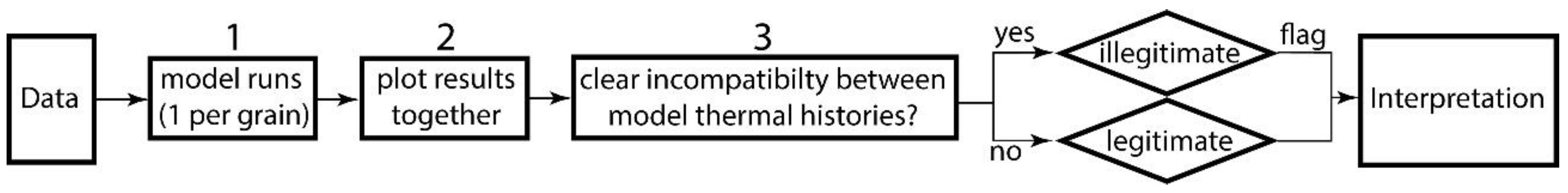
Figure 3.
Thermal model results for individual single grain runs from sample B5 of [12]. Red represents results for date rejected by [12]. Blue represents dates not rejected by [12]. Results are shown as accepted individual time-temperature paths from post “burn in” model iterations. The white arrow points to accepted red paths that overlap with the blue histories.
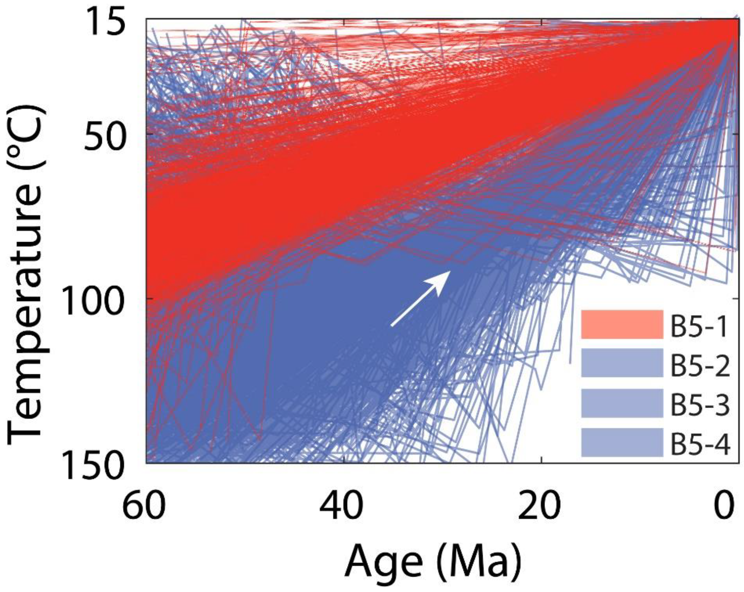
Figure 4.
(U-Th)/He date for sample B−5 plotted vs. grain size [12]. The biggest grain with the largest measured date was rejected based on a Q-test, even though the variation is legitimate because the closure temperature of the large grain is hotter than the smaller grains.
Figure 4.
(U-Th)/He date for sample B−5 plotted vs. grain size [12]. The biggest grain with the largest measured date was rejected based on a Q-test, even though the variation is legitimate because the closure temperature of the large grain is hotter than the smaller grains.
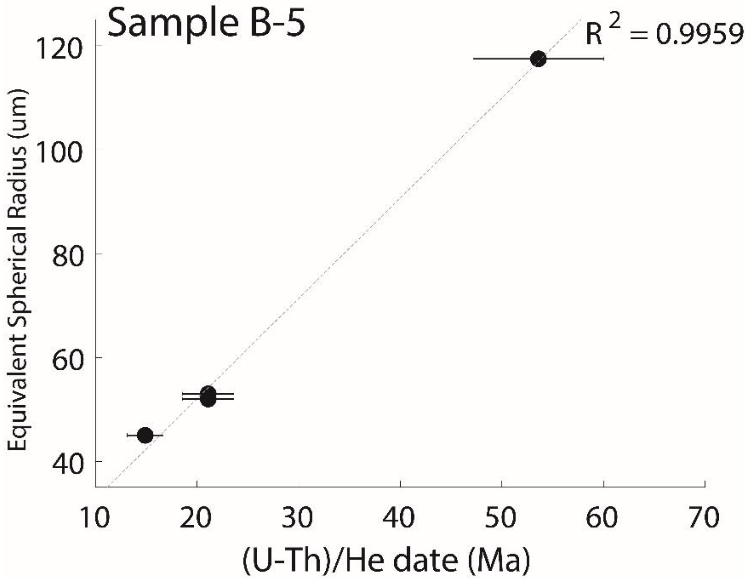
Figure 5.
Thermal model results for individual single grain runs from sample B2 of [12]. (A) Red represents results for date rejected by [12]. Blue represents dates not rejected by [12]. Results shown as accepted individual time-temperature paths from post “burn in” model iterations. (B) Same frame as shown in A with accepted post “burn in” thermal histories from model with all grains run together shown in green.
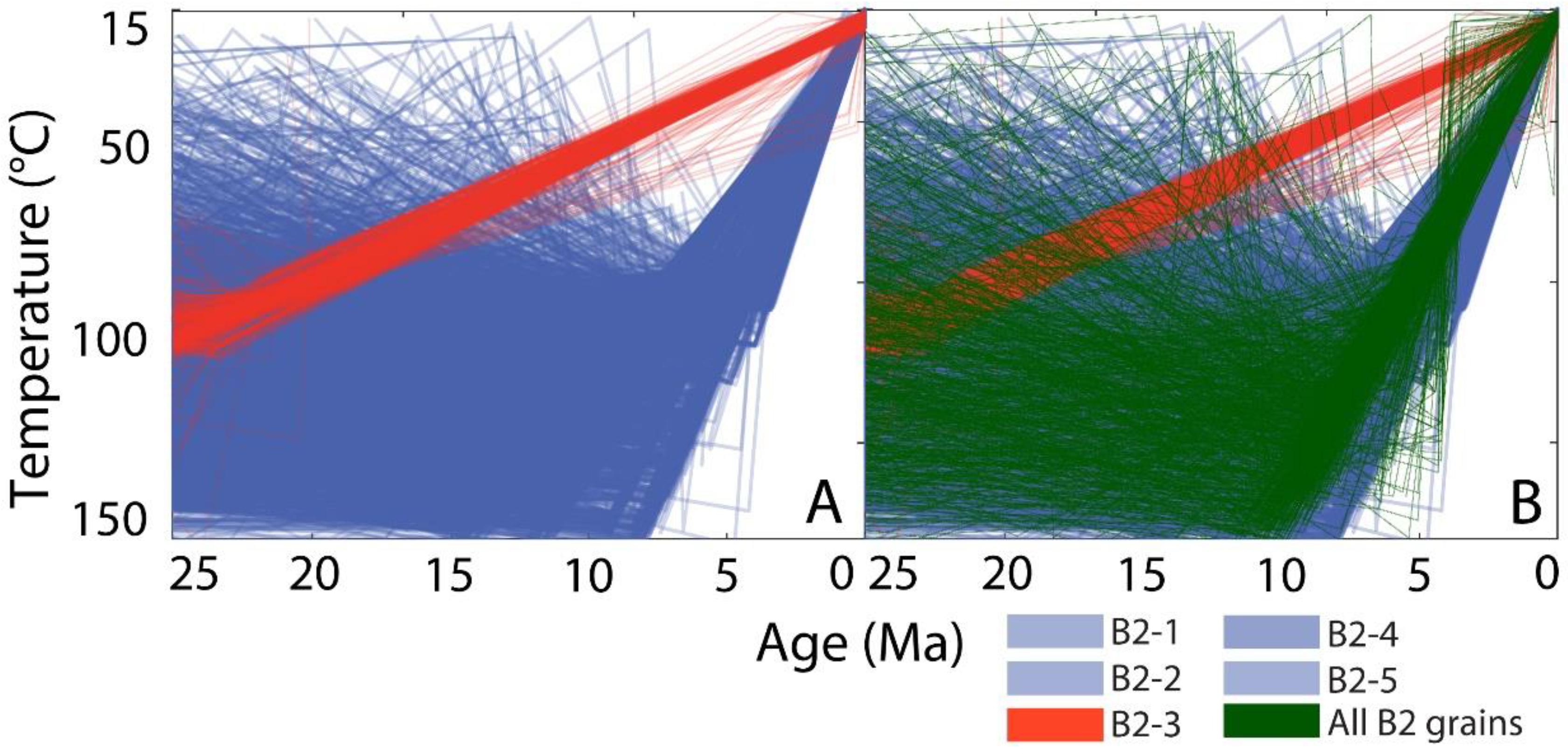
Figure 6.
Thermal model results for individual single grain runs from sample GP9S6 of [11]. (A). Red represents results for dates not rejected by [11]. Black and blue represent different groupings of dates all rejected by [11]. Results shown as accepted individual time-temperature paths from post “burn in” model iterations. (B) Same frame as in (A) but with accepted post “burn in” thermal histories from the aggregate 6 grains model shown in green.
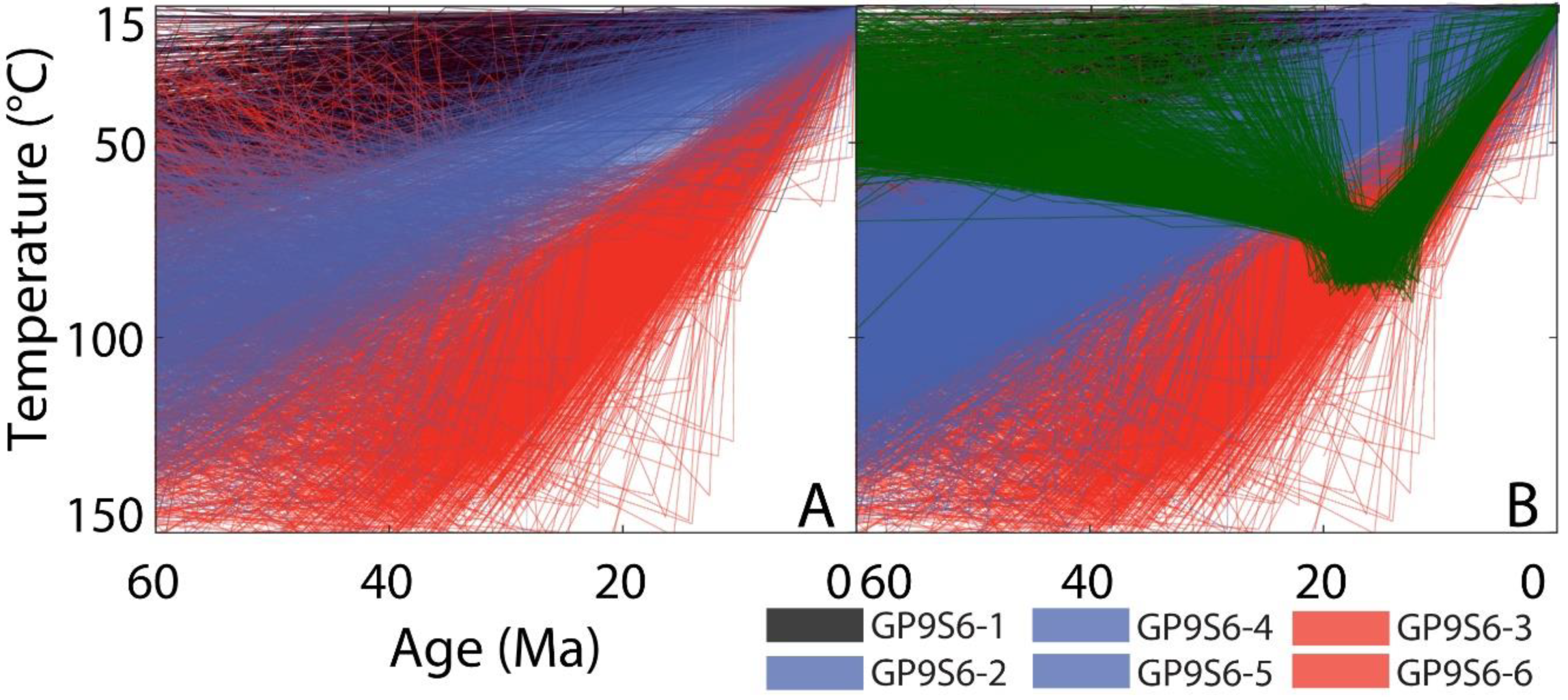
Figure 7.
Thermal model results for individual single grain runs from sample 11SS6 in [13]. No dates were rejected by [13]. Red represents the oldest grain (11SS6-b) and blue the youngest (11SS6-c) and are shown as accepted individual time-temperature paths from post “burn in” model iterations. The allowable thermal histories of the other 5 grains all are focused on the zone of overlap between these two and are plotted in gray beneath the blue and red. The low temperature constraint is shown as red box. The extent of this figure represents the time-temperature bounding box used in all model runs.


Table 1.
Synthetic data and corresponding forward model date from HeFTy. Each forward model date was computed by HeFTy using the input values of U, Th, Sm, grain size, and the following three-point thermal history: (1) 15 °C at 100 Ma, (2) 75 °C at 10 Ma, and (3) 15 °C at 0 Ma. ESR is equivalent spherical radius.
| Number | Forward Model Date (Ma) | U (ppm) | Th (ppm) | Sm (ppm) | ESR (μm) |
|---|---|---|---|---|---|
| 1 | 7.9 | 5 | 5 | 5 | 75 |
| 2 | 11.7 | 25 | 25 | 25 | 40 |
| 3 | 31.0 | 25 | 25 | 25 | 75 |
| 4 | 62.3 | 25 | 25 | 25 | 160 |
| 5 | 73.6 | 50 | 50 | 50 | 75 |
| 6 | 91.7 | 100 | 100 | 100 | 75 |
Table 2.
Apatite (U-Th)/He data. X in first column indicates that a date was rejected by its authors.
Table 2.
Apatite (U-Th)/He data. X in first column indicates that a date was rejected by its authors.
| Sample | Age (Ma) | Err 1 s (Ma) | U (ppm) | Th (ppm) | Sm (ppm) | He (ncc/mg) | Ft | ESR (μm) c | Lithology & Locale | |
|---|---|---|---|---|---|---|---|---|---|---|
| B2–1 | 3.98 | 0.02 | 112.1 | 3.66 | 2009 | 49.1 | 0.88 | 136 | Proterozoic schist [12] Greater Caucasus | |
| B2–2 | 4.28 | 0.03 | 77.45 | 3.46 | 1872 | 35.4 | 0.84 | 93.5 | ||
| X | B2–3 a | 14.89 | 0.1 | 91.69 | 3.8 | 1951 | 146.7 | 0.85 | 105 | |
| B2–4 | 4.94 | 0.04 | 62.06 | 1.75 | 164.6 | 30.9 | 0.82 | 84 | ||
| B2–5 | 3.03 | 0.03 | 99.04 | 3.44 | 229.7 | 29.8 | 0.8 | 82 | ||
| X | B5–1 a | 53.61 | 3.22 | 106.7 | 1.78 | 200.9 | 590.0 | 0.85 | 117.5 | Proterozoic igneous rocks [12] Greater Caucasus |
| B5–2 | 14.87 | 0.89 | 63.12 | 2.94 | 108.8 | 83.6 | 0.72 | 45 | ||
| B5–3 | 21.12 | 1.27 | 192.6 | 11.62 | 198.7 | 371.6 | 0.74 | 52 | ||
| B5–4 | 21.11 | 1.27 | 67.65 | 1.87 | 169 | 132.2 | 0.75 | 53 | ||
| X | GP9S6–1 b | 60.1 | 3 | 22.1 | 80.5 | 200.3 | 239.1 | 0.75 | 61 c | Protero-Paleozoic granitoids and metamorphic rocks [11] Shillong Plateau (India) |
| X | GP9S6–2 b | 24.3 | 1.2 | 22.4 | 97.2 | 1065 | 104.2 | 0.65 | 43.5 c | |
| GP9S6–3 | 9.9 | 0.5 | 16.2 | 81.7 | 877.5 | 33.3 | 0.65 | 43.5 c | ||
| X | GP9S6–4 b | 26.7 | 1.3 | 15 | 48.7 | 210.5 | 59 | 0.69 | 49 c | |
| X | GP9S6–5 b | 30.3 | 1.5 | 14.4 | 45 | 531.5 | 59.3 | 0.64 | 41.5 c | |
| GP9S6–6 | 10 | 0.6 | 7.1 | 35.6 | 690.7 | 15.7 | 0.64 | 42.5 c | ||
| 11SS6–a | 98.0 | 3.3 | 19.1 | 21.1 | 62.3 | 210.6 | 0.73 | 54 c | Cretaceous granitoid [13] Western Sierra Nevada Foothills (California) | |
| 11SS6–b | 112.6 | 4.9 | 19.7 | 22.6 | 55.4 | 224.0 | 0.65 | 41 c | ||
| 11SS6–c | 81.2 | 3.5 | 20.0 | 29.0 | 60.9 | 168.0 | 0.63 | 40 c | ||
| 11SS6–d | 86.9 | 3.2 | 51.4 | 63.4 | 114.4 | 459.2 | 0.65 | 41 c | ||
| 11SS6–e | 86.5 | 2.9 | 16.0 | 23.1 | 56.5 | 165.8 | 0.72 | 52 c | ||
| 11SS6–f | 83.2 | 2.8 | 29.3 | 43.1 | 76.4 | 286.7 | 0.71 | 50 c | ||
| 11SS6–g | 93.1 | 2.8 | 35.0 | 52.6 | 84.0 | 392.0 | 0.72 | 52 c |
Publisher’s Note: MDPI stays neutral with regard to jurisdictional claims in published maps and institutional affiliations. |
© 2020 by the authors. Licensee MDPI, Basel, Switzerland. This article is an open access article distributed under the terms and conditions of the Creative Commons Attribution (CC BY) license (http://creativecommons.org/licenses/by/4.0/).
Share and Cite
MDPI and ACS Style
Sousa, F.J.; Farley, K.A. A Framework for Evaluating Variation in (U-Th)/He Datasets. Minerals 2020, 10, 1111. https://doi.org/10.3390/min10121111
AMA Style
Sousa FJ, Farley KA. A Framework for Evaluating Variation in (U-Th)/He Datasets. Minerals. 2020; 10(12):1111. https://doi.org/10.3390/min10121111
Chicago/Turabian StyleSousa, Francis J., and Kenneth A. Farley. 2020. "A Framework for Evaluating Variation in (U-Th)/He Datasets" Minerals 10, no. 12: 1111. https://doi.org/10.3390/min10121111
Note that from the first issue of 2016, this journal uses article numbers instead of page numbers. See further details here.