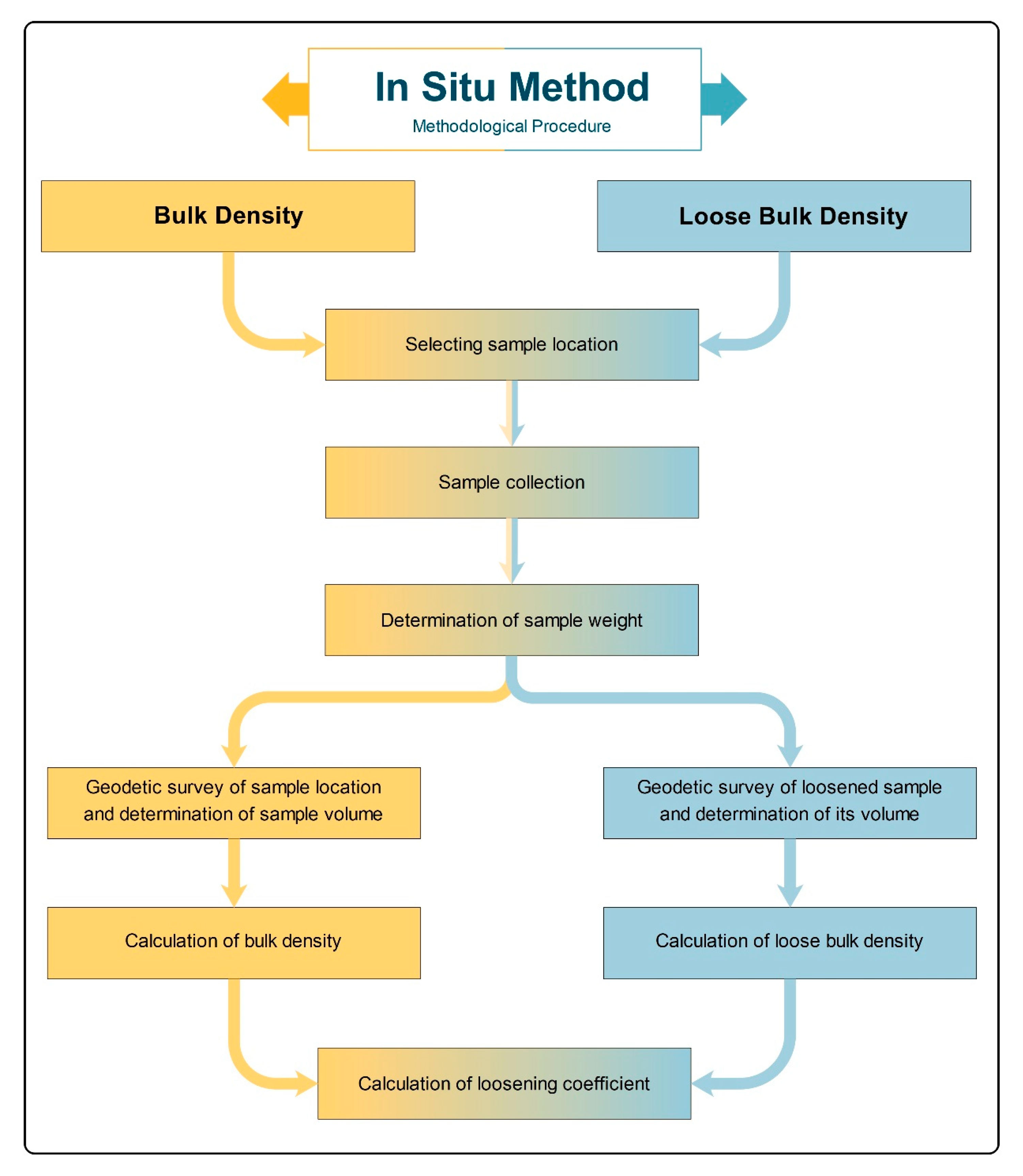
The in situ method is the determination of bulk density from direct field measurements. In this case, it is important to take a sample with the highest volume possible, ideally around 10 m3, but at least 1 m3. A sample of rock material in the natural state with a volume of 5 to 7 m3 is usually sufficient for objective determination of bulk density. In the field determination of bulk density, the aim is generally to collect as much raw material as possible, that can be weighed together with the vehicle, by one weighing, without further manipulation (loading, unloading, emptying, etc.). A sufficient sample size reduces the bulk density error due to the heterogeneity of the raw material. Thus, the larger the volume entering the measurement, the more representative the resulting bulk density will be. The weighing of the sample taken shall be carried out on a certified weight immediately after sampling to avoid drying or wetting of the sample due to climatic conditions. The volume of the sample taken for field bulk density determination is then determined using geodetic or photogrammetric methods. The bulk density itself is then calculated according to (1) as the ratio of the mass of the large-scale sample to its volume from the data determined directly in the field.
2.4.2. Geodetic Survey of Samples Location and Determination of Their Volume in Situ
There are several geodetic methods and technologies, such as tacheometry, grid leveling, photogrammetry, laser scanning, or GNSS methods, which can be implemented to determine the shape of a body—the volume of the stock or volume of a material sample. In practice, terrestrial laser scanning, digital photogrammetry, and GNSS methods are currently most commonly used. For purposes of this research, terrestrial laser scanning was chosen as the most accurate and effective technology and digital close-range photogrammetry as the comparative method.
Terrestrial Laser Scanning (TLS)
TLS measurements were performed in the coordinate system Datum of Uniform Trigonometric Cadastral Network (S-JTSK) and vertical datum Baltic Vertical Datum—After Adjustment (Bpv). These are obligatory systems used in Slovakia. Nail survey marks, as temporary monumented points with respect to the operation of the quarry, were used as reference points. The approximate coordinates and heights of these points were determined by the RTK (real-time kinematic) method using the Leica GPS900CS GNSS instrument (Leica Geosystems AG, Heerbrugg, Switzerland) connected to a network of SKPOS (Slovak real-time positioning service) reference stations. The horizontal accuracy of the coordinates of the points determined in this way (guaranteed by the SKPOS service) is usually up to ±20 mm and vertical ±40 mm with respect to the measurement conditions. The resulting coordinates of the survey net points were determined by the spatial polar method using a total station Leica TS 02 (Leica Geosystems AG, Heerbrugg, Switzerland) with an internal accuracy in the survey net of up to 2 mm.
The method of the temporary station was used to determine the coordinates of HDS (High Definition Survey) targets used for TLS. The Leica TS 02 instrument was used for the measurement. The technical specification of this instrument gives an angular accuracy (horizontal and vertical) of 1.5 mgon. The length measurement accuracy is 2 mm + 2 ppm according to the manufacturer in standard measurement mode. The Leica GMP 111 surveying prism was used for the orientation. The Leica HDS 6” circular tilt & turn targets placed on a tripod were used as ground control points (GCP) for laser scanning. Their coordinates were determined by the spatial polar method.
The horizontal accuracy of the polar method is expressed by the mean positional error
mp of the coordinates of the measured point according to the equation:
where:
mpA—mean positional error of the instrument’s survey station,
s—slope distance,
z—zenithal distance,
mω—mean error of the observed direction,
mz—mean error of the observed zenithal distance,
ms—mean error of the measured length,
ρ—conversion coefficient.
The vertical accuracy is determined by the mean error derived for trigonometrical measurement of heights by the equation:
where:
The internal accuracy is calculated as a priori mean error of measurement for the furthest measured points from the survey station (assuming s = 80 m, z = 105 g) as mp ≤ 10 mm and mh = ≤ 10 mm.
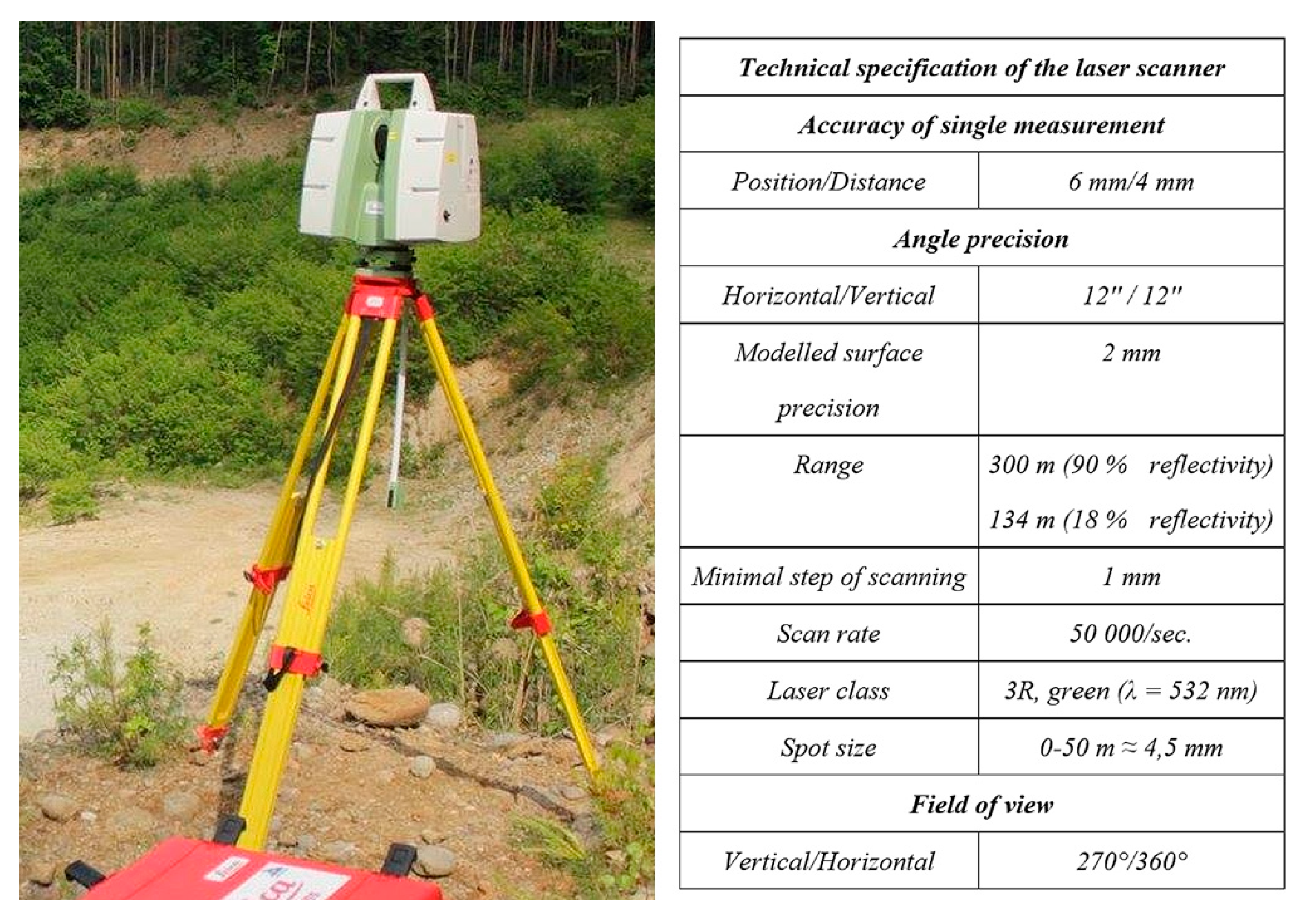
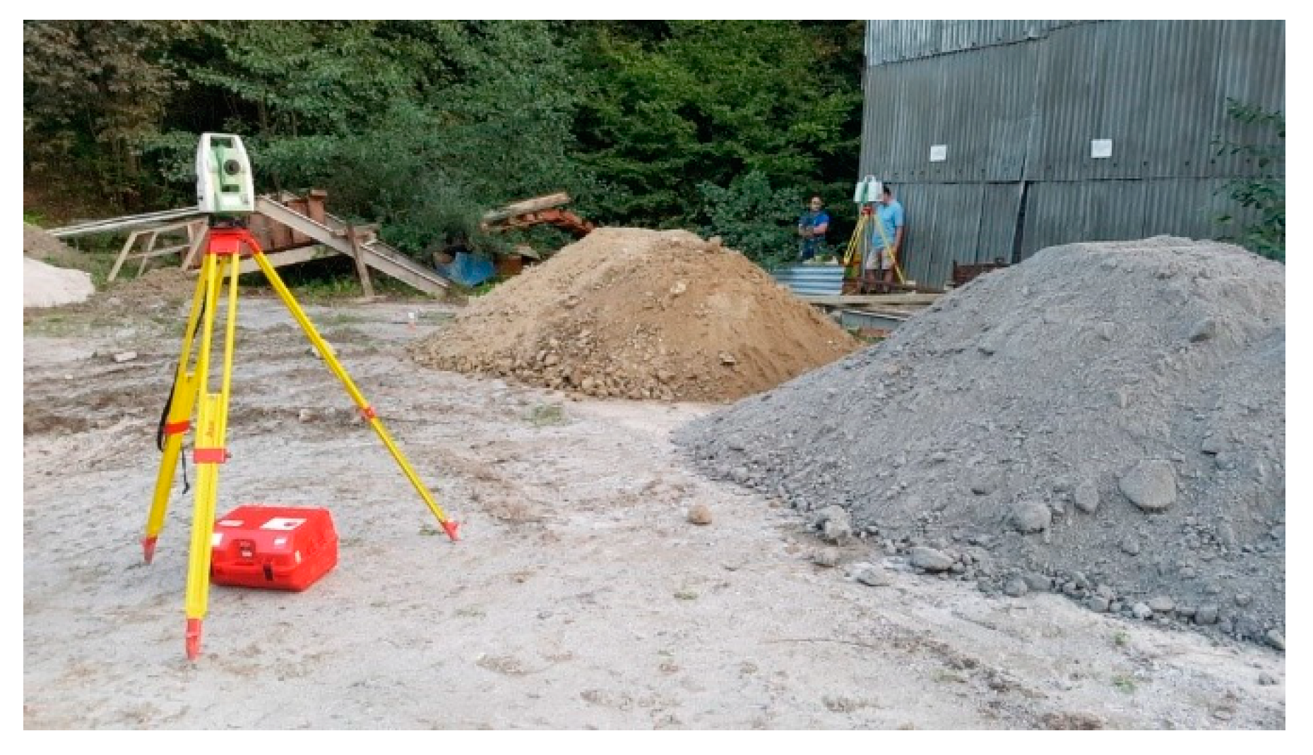
The Leica ScanStation C10 laser scanner (Leica Geosystems AG, Heerbrugg, Switzerland) was used to measure and determine the volume of large-scale samples of the raw material in the natural state (
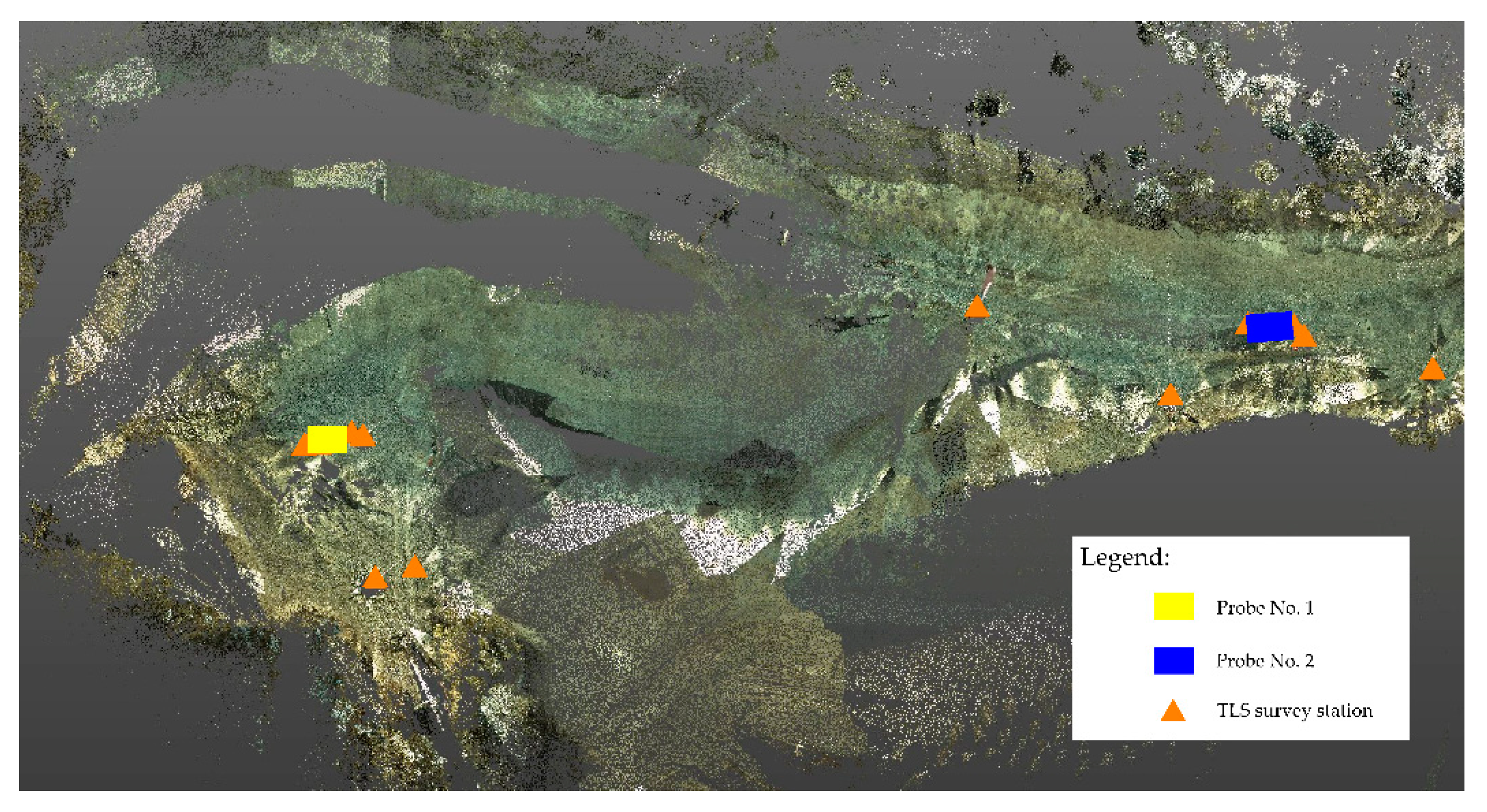
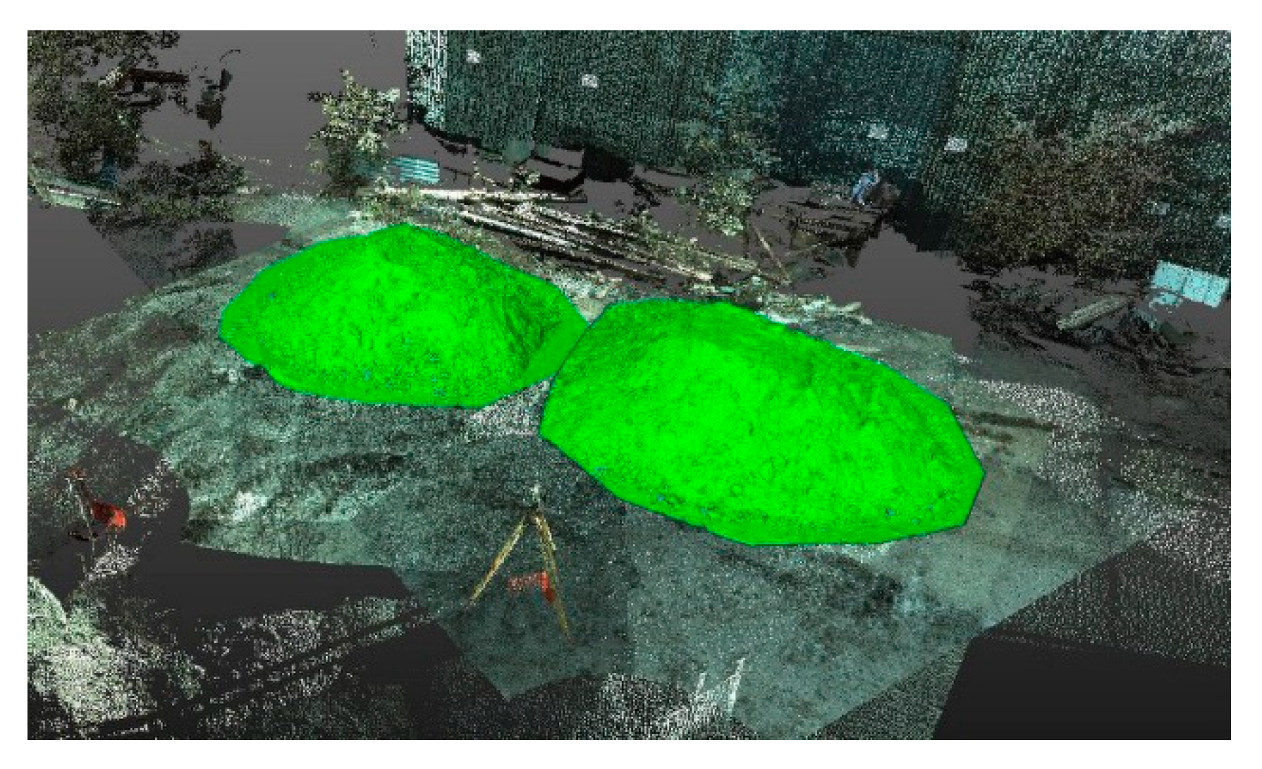
Figure 8). The scanner uses a pulse laser distance meter with 532 nm wavelength and class 3R with green visible light for length measurements. Partial scans were mutually registered by direct georeferencing in the S-JTSK coordinate system using the ground control points with Leica HDS targets (
Figure 9). The accuracy of registration is derived from the intersection residues. Its value was up to
mp = ±2 mm. The point density setting for laser scanning was set as 10 mm at a distance of 30 m, both horizontally and vertically. The initial point cloud from scanning contained 1.20/0.8 mil. points for both probes. In postprocessing, the overlapped scans were registered together and spatially filtered for a 10 mm point spacing due to the granularity and physical properties of the raw material. The resampled point cloud used for calculations contained approximately 163,000/143,000 points.
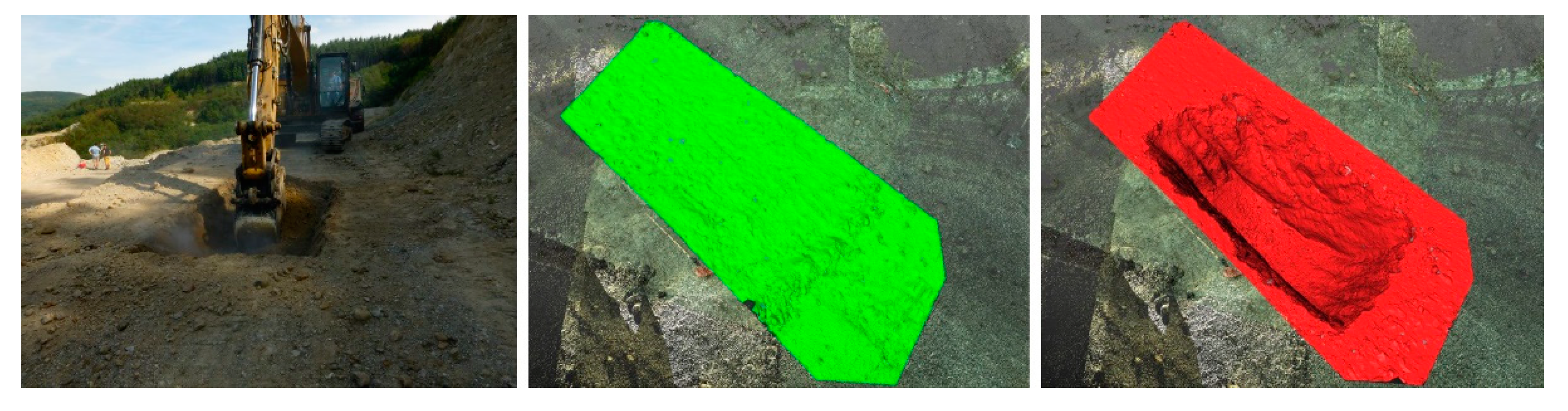
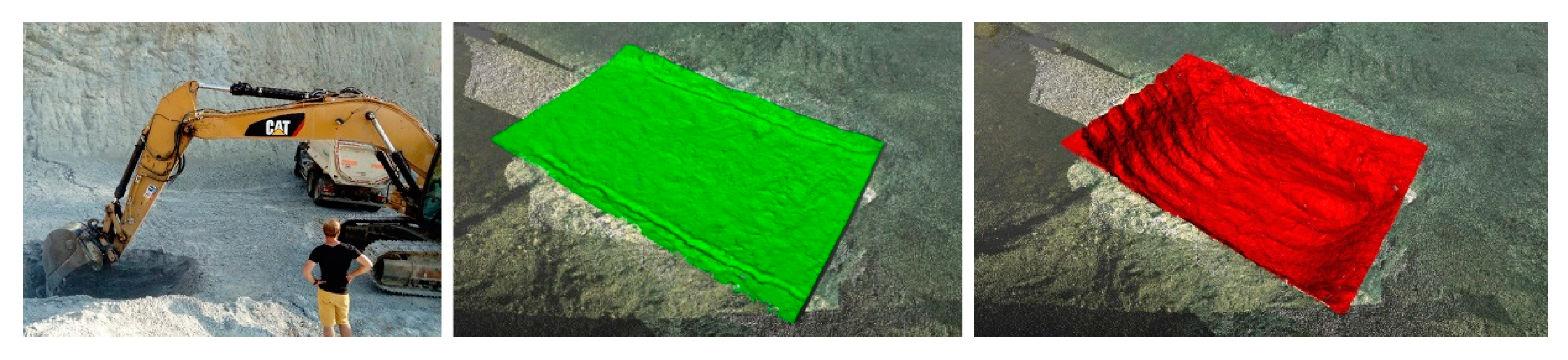
The TLS measurements resulted in a dense point cloud from which TIN models of individual surfaces were generated—always before and after excavation. The volume of the excavated raw material—the large-scale sample was determined by the difference between the two TIN models.
Digital Close-Range Photogrammetry
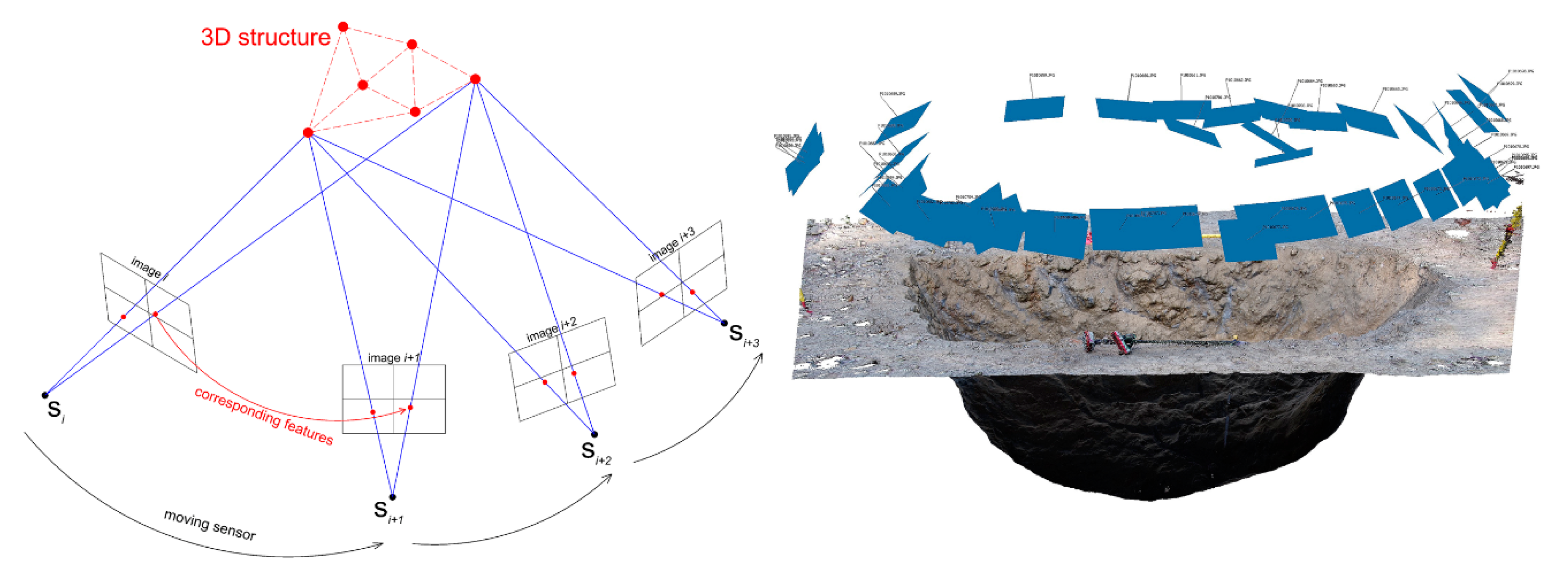
Photogrammetric measurement of large-scale samples was performed after excavation, using the “Structure from Motion” (SfM) method. The SfM method represents one of the most advanced approaches in photogrammetric image processing and is based on estimating the 3D structure of 2D sequences of digital images that are associated with the movement of the used recording medium – digital camera (
Figure 10). The principle of the method is based on biological vision, thanks to which people can reconstruct the spatial structure of their surroundings from a 2D image perceived and projected onto the retina. Essentially, it can be characterized as the combination of stereophotogrammetry and convergence case of photogrammetry—i.e., the possibility to use images with both parallel and convergent axes. The big advantage of this method is the automated image processing and simultaneous determination of the elements of the interior and exterior orientation of the camera and the 3D structure on the images [
33].
Photogrammetric imaging was performed using an Olympus PEN E-PL5 digital camera (Olympus Corporation, Tokyo, Japan) with a focal length of 14 mm, aperture f/6.3 and ISO 200, from a distance of about 3.7 m and without using a tripod. Subsequent image processing was performed in Agisoft PhotoScan® Professional Edition, Version 1.2 software (Agisoft LLC, St. Petersburg, Russia).
Trimble RealWorks® Version 10.0.4.441 software (Trimble Inc., Sunnyvale, CA, USA) was used to calculate the volume of large-scale samples. Using this software, the volume of large-scale samples (excavated pit) was determined using the two-volume calculation function (upper and lower surface).
Table 3 shows the volumes of large-scale samples—Probe 1 and 2.
To verify the accuracy of the measurements and calculation of sample volume from the TLS measurements, an alternative measurement using the close-range photogrammetry (SfM method) was also performed. The resulting data from photogrammetric processing were subsequently used to create control 3D models for independent-control calculation of the volume of large-scale samples. The results of the control calculation are given in
Table 3. It shows that the calculations differ only insignificantly—by less than 2 percent of the volume. This is also consistent with the results from the differential models created for the large-scale samples.
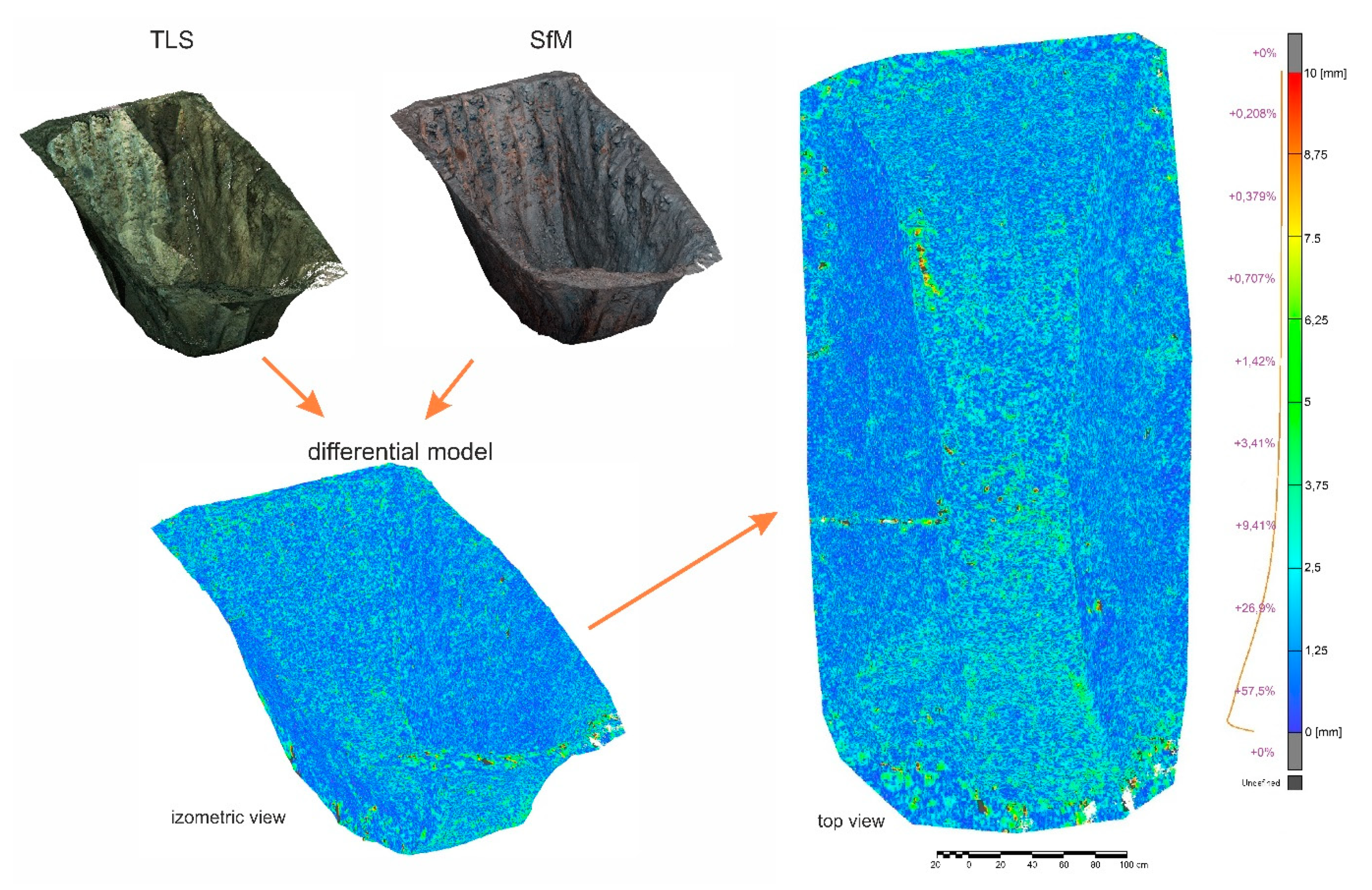
The photogrammetric processing of both large-scale samples resulted in a dense point cloud with an assigned RGB texture from the images. The point clouds of both probes were then compared with the point clouds obtained by terrestrial laser scanning. This was done by means of a differential model determining the spatial variation of the two compared models (
Figure 11). The model was generated in the
3DReshaper 2018 Version 18.0 software (Leica Geosystems AG, Heerbrugg, Switzerland) using the compare/inspect function, which is used to determine robust distances between two point clouds. The different models show that the distances between the two clouds reach the maximum value of 9.5 mm with the mean value of deviations at 1.6 mm. Overall, 99% of the deviations are between 0 and 6.25 mm.
The statistics of the process of measuring the shape and volume of large-scale samples by the close-range photogrammetry and the results of the photogrammetric processing by the SfM method are given in
Table 4.
Based on the results obtained by both methods, it can be concluded that the control measurement by the SfM photogrammetry method gives comparable results in terms of accuracy. However, the comparable accuracy has been achieved for the given averaged scanning/imaging distance (approx. 4 m in our case), respectively for comparable distances, as the achievable accuracy of photogrammetric processing decreases as the imaging distance increases (while laser scanning achieves guaranteed accuracy within the range of the instrument) [
35].
Results of photogrammetric processing, unlike TLS, provide a higher density of the resulting point clouds. Moreover, thanks to better “maneuverability” with the camera, it is possible to capture even areas that may remain obscured during scanning, and their absence in the resulting model can lead to distorted results. On the other hand, photogrammetric imaging is sensitive to light conditions and, in the case of insufficient illumination of the measured surface (or significantly varying illumination during imaging), subsequent processing of the images can be problematic as well as lead to incorrect results.

 ,
, 


