
Application of Airborne Magnetic Survey in Deep Iron Ore Prospecting—A Case Study of Jinling Area in Shandong Province, China

 , ,
, ,
Abstract
:1. Introduction
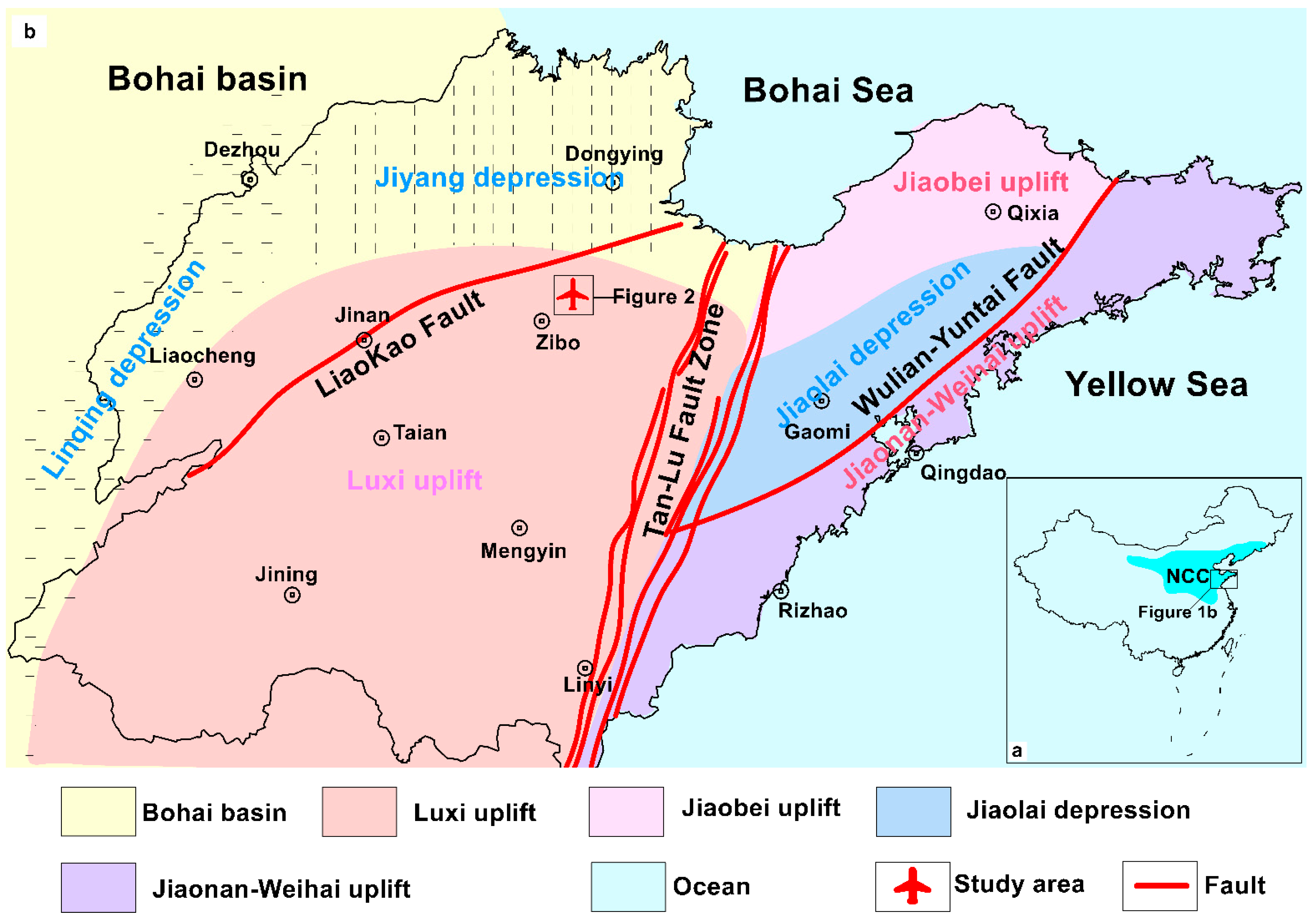
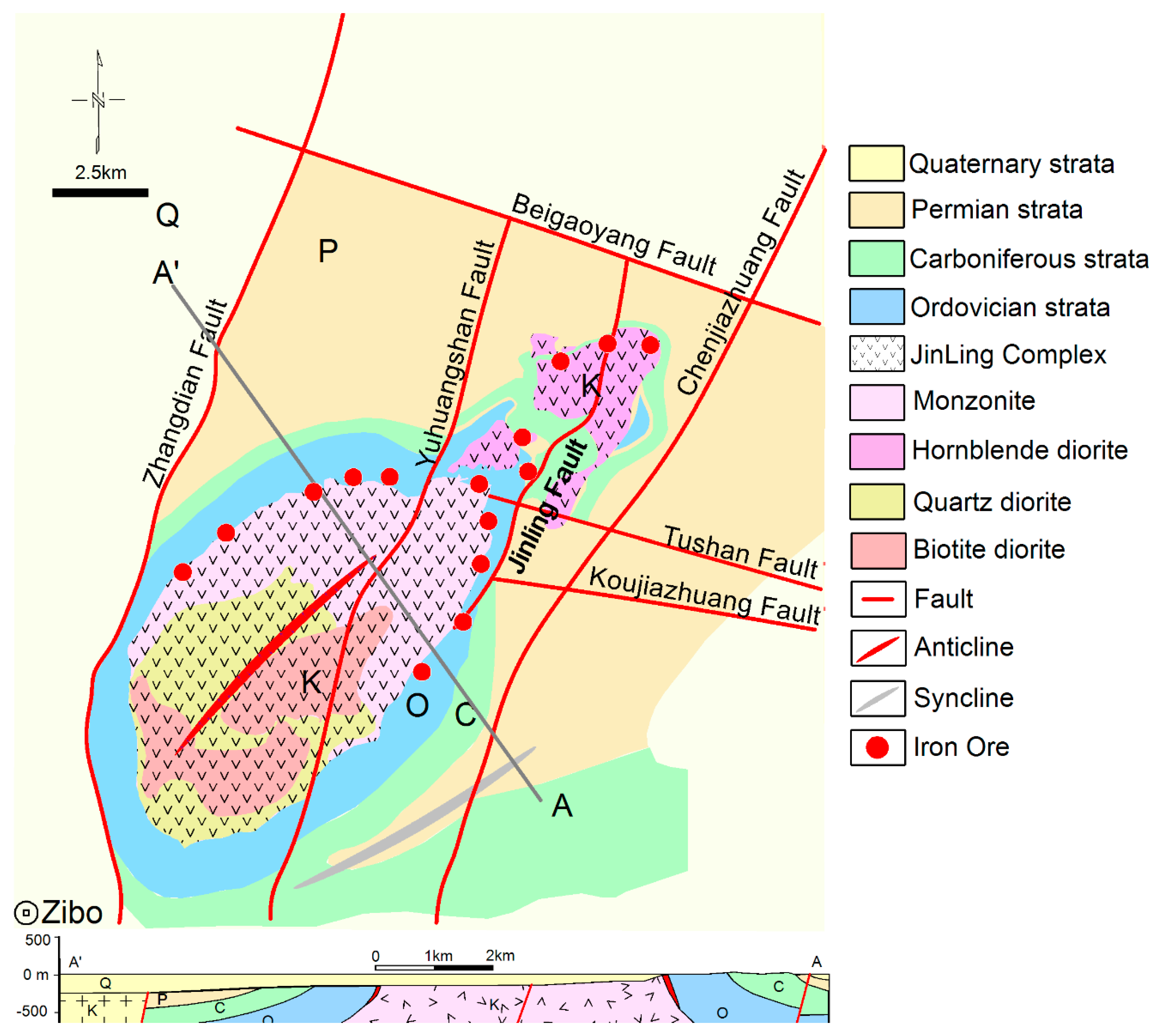
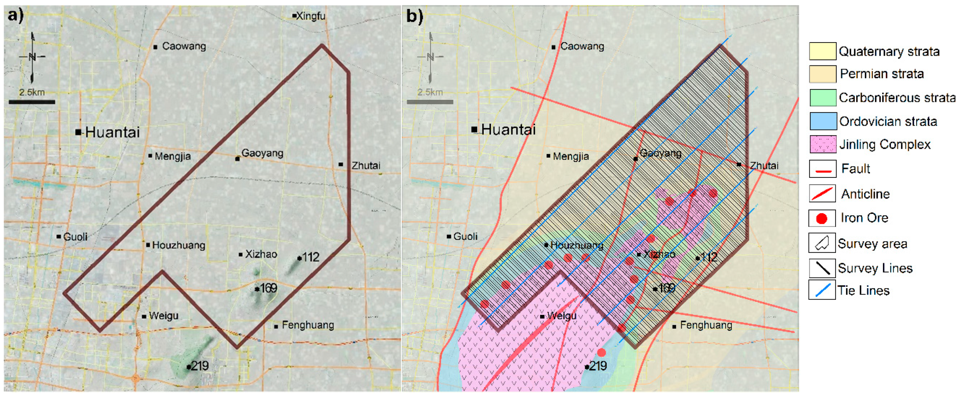
2. Regional Geology
3. Airborne Magnetic Survey
3.1. Airborne Magnetic Survey System
3.2. Survey Flight
3.2.1. Survey Lines
3.2.2. Test Flight
- (1)
- Compensation and Heading Error Test
- (2)
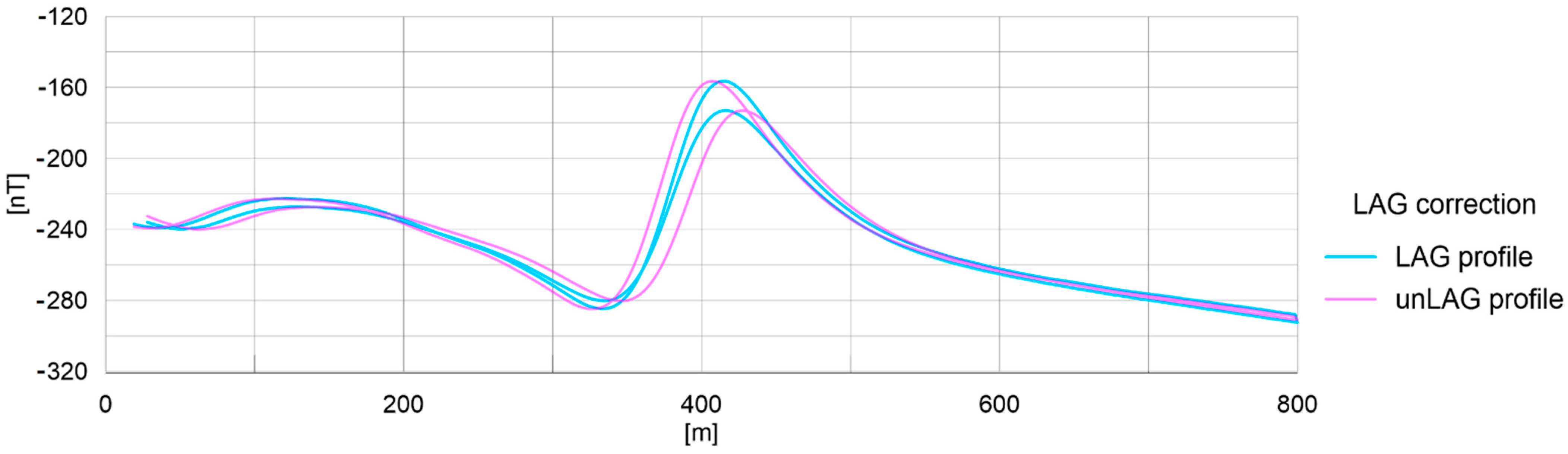
- LAG Test
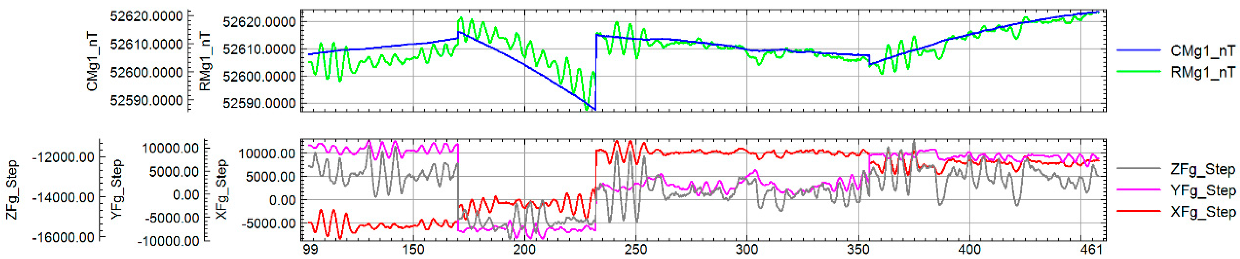
3.2.3. Corrections
- (1)
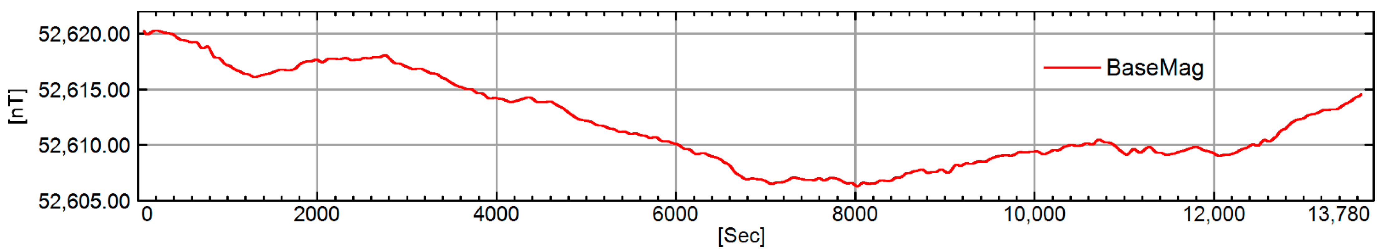
- Diurnal Magnetic Correction
- (2)
- Lag Correction
- (3)
- Background Removal
3.3. Data Processing
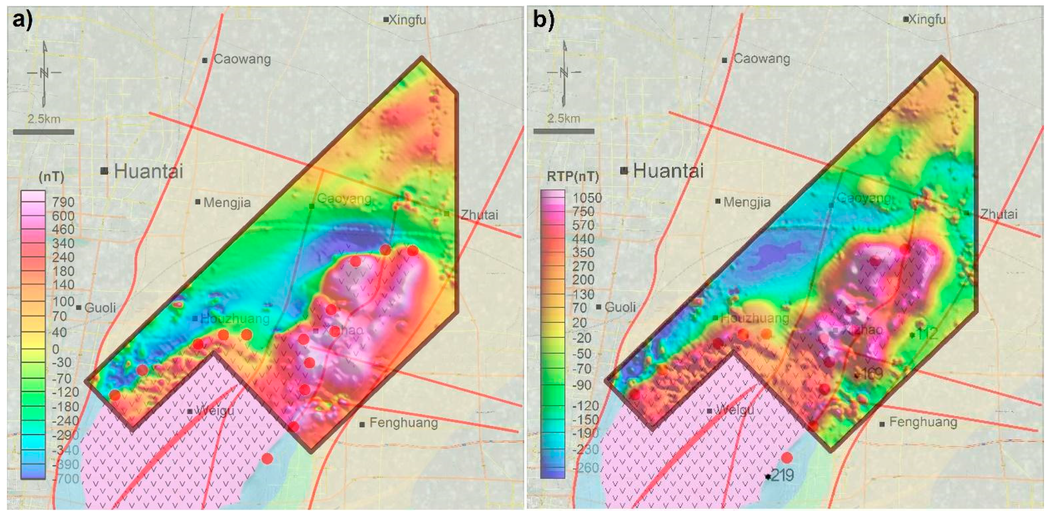
3.3.1. Reduction to the Magnetic Pole
3.3.2. Low Pass Filter
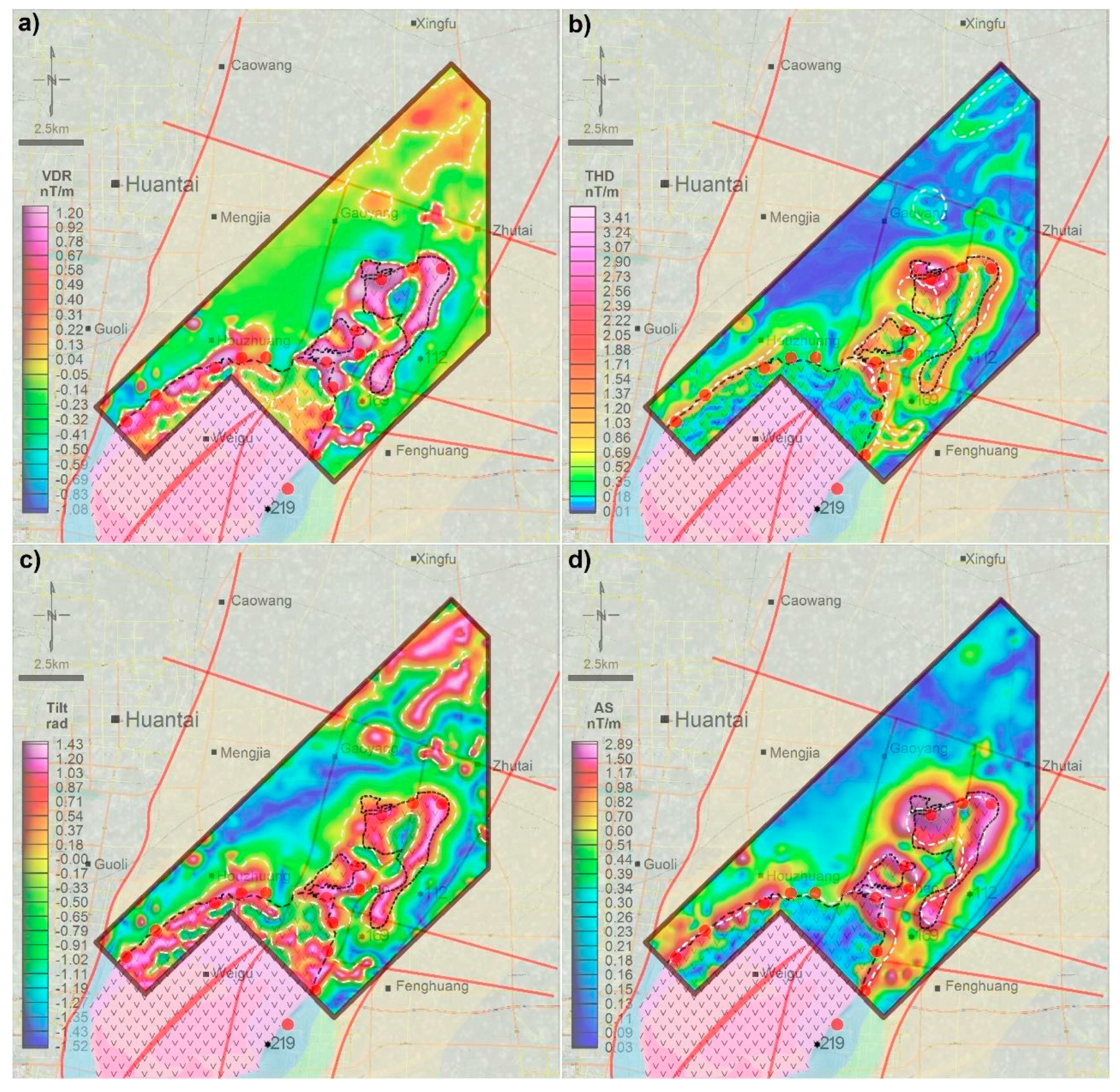
3.3.3. Boundary Enhancement and Edge Detection
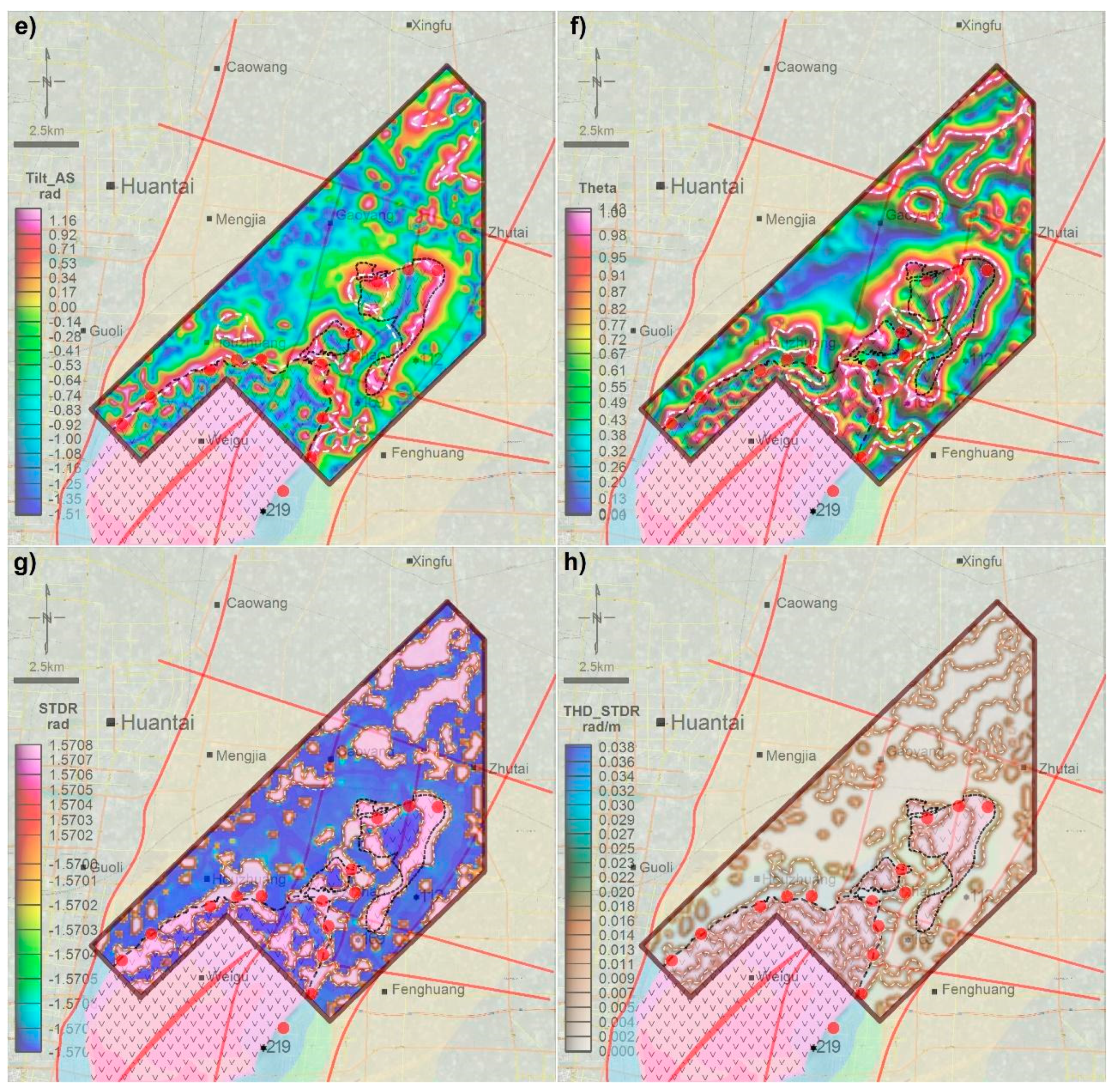
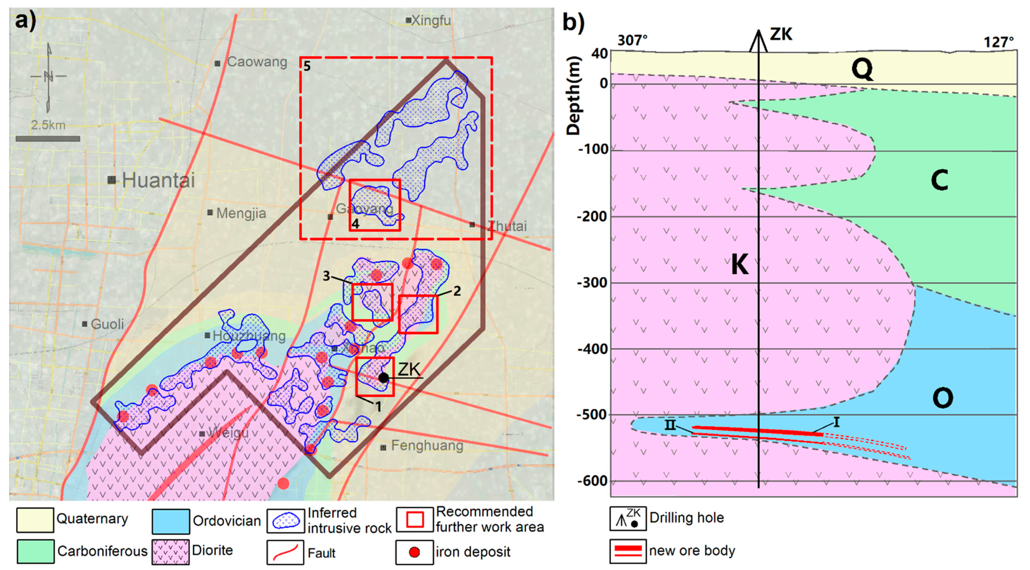
4. Results and Discussion
5. Conclusions
Author Contributions
Funding
Acknowledgments
Conflicts of Interest
References
- Nabighian, M.N.; Grauch, V.J.S.; Hansen, R.O.; LaFehr, T.R.; Li, Y.; Peirce, J.W.; Phillips, J.D.; Ruder, M.E. The Historical Development of the Magnetic Method in Exploration. Geophysics 2005, 70, 33ND–61ND. [Google Scholar] [CrossRef]
- Viberg, A.; Trinks, I.; Lidén, K. A Review of the Use of Geophysical Archaeological Prospection in Sweden. Archaeol. Prospect. 2011, 18, 43–56. [Google Scholar] [CrossRef]
- Logachev, A.A.; Hawkes, H.E. The Development and Applications of Airborne Magnetometers in the U.S.S.R. Geophysics 1946, 11, 135–147. [Google Scholar] [CrossRef]
- Bubner, G.; Hills, R.; Dhu, T.; Dentith, M. Geophysical Exploration for Iron Ore in the Middleback Ranges, South Australia. ASEG Ext. Abstr. 2003, 2003, 29–46. [Google Scholar] [CrossRef]
- Abulghasem, Y.A.; Akhir, J.M.; Samsudin, A.R.; Hassan, W.F.W.; Youshah, B.M. Integrated Data of Remote Sensing and Geophysical Data for Iron Ore Exploration in the Western Part of Wadi Shatti District, Libya. EJGE 2011, 16, 1441–1454. [Google Scholar]
- CunnInGhaM, M.I.C.; De Waele, B. Geological Mapping of Badondo and Iron Mineralisation Targets, Republic of Congo. Struct. Geol. Resour. 2012, 2012, 54–56. [Google Scholar]
- Mieth, M.; Jokat, W. Banded Iron Formation at Grunehogna Craton, East Antarctica—Constraints from Aeromagnetic Data. Precambrian Res. 2014, 250, 143–150. [Google Scholar] [CrossRef]
- Leao-Santos, M.; Li, Y.; Moraes, R. Application of 3D Magnetic Amplitude Inversion to Iron Oxide-Copper-Gold Deposits at Low Magnetic Latitudes: A Case Study from Carajas Mineral Province, Brazil. Geophysics 2015, 80, B13–B22. [Google Scholar] [CrossRef]
- Oladunjoye, M.A.; Olayinka, A.I.; Alaba, M.; Adabanija, M.A. Interpretation of High Resolution Aeromagnetic Data for Lineaments Study and Occurrence of Banded Iron Formation in Ogbomoso Area, Southwestern Nigeria. J. Afr. Earth Sci. 2016, 114, 43–53. [Google Scholar] [CrossRef]
- Mazhari, N.; Shafaroudi, A.M.; Ghaderi, M. Detecting and Mapping Different Types of Iron Mineralization in Sangan Mining Region, NE Iran, Using Satellite Image and Airborne Geophysical Data. Geosci. J. 2017, 21, 137–148. [Google Scholar] [CrossRef]
- Ives, B.T.; Mickus, K. Using Gravity and Magnetic Data for Insights into the Mesoproterozoic St. Francois Terrane, Southeast Missouri: Implications for Iron Oxide Deposits. Pure Appl. Geophys. 2019, 176, 297–314. [Google Scholar] [CrossRef]
- Raju, P.V.S.; Kumar, K.S. Magnetic Survey for Iron-Oxide-Copper-Gold (IOCG) and Alkali Calcic Alteration Signatures in Gadarwara, M.P, India: Implications on Copper Metallogeny. Minerals 2020, 10, 671. [Google Scholar] [CrossRef]
- Voll, E.; Silva, A.M.; Pedrosa-Soares, A.C. Tracking Iron-Rich Rocks beneath Cenozoic Tablelands: An Integration of Geological, Airborne Geophysical and Remote Sensing Data from Northern Minas Gerais State, SE Brazil. J. S. Am. Earth Sci. 2020, 101, 102604. [Google Scholar] [CrossRef]
- Harikumar, P.; Rajaram, M.; Balakrishnan, T.S. Aeromagnetic Study of Peninsular India. Proc. Indian Acad. Sci. Earth Planet. Sci. 2000, 109, 381–391. [Google Scholar] [CrossRef] [Green Version]
- Yao, P. Records of China’s Iron Ore Deposits; Metallurgic Industry Press: Beijing, China, 1993; ISBN 978-7-5024-1449-8. [Google Scholar]
- Changchun, Y.; Zhengguo, F.; Naidong, Y.; Shengqing, X.; Jianhua, W.; Hongrui, Z. High-resolution aeromagnetic exploration methods and their application in daye iron mines. Prog. Geophys. 2007, 22, 979–983. [Google Scholar]
- Minan, W.; Qingsong, W.; Guangwen, Z.; Xiaobin, C.; Shixue, Y.; Qinson, D. Discovery of the Nihe Iron Deposit in Lujiang, Anhui, and its Exploration Significance. Acta Geol. Sin. 2011, 85, 802–809. [Google Scholar]
- Teng, S.; Wen, D.; Hong, X.; Zhang, H. Perspective resources estimated by comprehensive information technology for the Dataigou iron deposit in Liaoning province. Geol. Resour. 2013, 22, 199–203. [Google Scholar]
- Wang, F.; Li, W. Application of MT method to anomly recognition during deep iron ore prospecting in Qian′an iron ore. Contrib. Geol. Miner. Resour. Res. 2013, 28, 604–612. [Google Scholar]
- Fan, Z.; Huang, X.; Yang, X.; Zhou, D.; Liu, Q. Aeromagnetic Exploration of Deep Iron Ore in Daye, China. Acta Geol. Sin. Engl. Ed. 2014, 88, 1233–1234. [Google Scholar] [CrossRef]
- Zhang, J.; Zeng, Z.; Zhao, X.; Li, J.; Zhou, Y.; Gong, M. Deep Mineral Exploration of the Jinchuan Cu–Ni Sulfide Deposit Based on Aeromagnetic, Gravity, and CSAMT Methods. Minerals 2020, 10, 168. [Google Scholar] [CrossRef] [Green Version]
- Zhao, Y. Main genetic types and geological characteristics of iron-rich ore deposits in China. Miner. Depos. 2013, 32, 686–705. [Google Scholar] [CrossRef]
- Zhao, Y.; Feng, C.; Li, D. The Major Ore Clusters of Super-Large Iron Deposits in the World, Present Situation of Iron Resources in China, and Prospect. Acta Geol. Sin. Engl. Ed. 2014, 88, 1895–1915. [Google Scholar] [CrossRef]
- General Administration of Customs of the People’s Republic of China Review of China’s Foreign Trade in 2019. Available online: http://english.customs.gov.cn/Statics/f63ad14e-b1ac-453f-941b-429be1724e80.html (accessed on 20 September 2020).
- Wu, J. Deep-felt consideration and important decision—The issue of “the Program Of Superseding Resources Prospecting in Crisis Mines in China (2004–2010)”. Resour. Ind. 2005, 7, 25–26. [Google Scholar]
- Liu, Y.; Yan, J.; Wu, M.; Zhao, W.; Zhao, J.; Deng, Z. Exploring Deep Concealed Ore Bodies Based on Gravity Anomaly Separation Methods: A Case Study of the Nihe Iron Deposit. Diqiu Wuli Xuebao 2012, 55, 4181–4193. [Google Scholar] [CrossRef]
- Liu, S.; Hu, X.; Cai, J.; Li, J.; Shan, C.; Wei, W.; Han, Q.; Liu, Y. Inversion of Borehole Magnetic Data for Prospecting Deep-Buried Minerals in Areas with near-Surface Magnetic Distortions: A Case Study from the Daye Iron-Ore Deposit in Hubei, Central China. Near Surf. Geophys. 2017, 15, 298–310. [Google Scholar] [CrossRef]
- Liu, S.; Hu, X.; Zhu, R. Joint Inversion of Surface and Borehole Magnetic Data to Prospect Concealed Orebodies: A Case Study from the Mengku Iron Deposit, Northwestern China. J. Appl. Geophys. 2018, 154, 150–158. [Google Scholar] [CrossRef]
- Shi, R.; Zhang, Y.; Lu, M.; Kuang, H.; Zhang, G. 3D Metallogenic Prediction Based on Geological and Gravity-magnetic Data Integration in the Qian’an Iron Ore Concentration Area, Hebei Province. Acta Geosci. Sin. 2018, 39, 762–770. [Google Scholar]
- Liu, S.; Fedi, M.; Hu, X.; Ou, Y.; Baniamerian, J.; Zuo, B.; Liu, Y.; Zhu, R. Three-Dimensional Inversion of Magnetic Data in the Simultaneous Presence of Significant Remanent Magnetization and Self-Demagnetization: Example from Daye Iron-Ore Deposit, Hubei Province, China. Geophys. J. Int. 2018, 215, 614–634. [Google Scholar] [CrossRef]
- Sun, S.; Chen, C.; Liu, Y. Constrained 3D Inversion of Magnetic Data with Structural Orientation and Borehole Lithology: A Case Study in the Macheng Iron Deposit, Hebei, China. Geophysics 2019, 84, B121–B133. [Google Scholar] [CrossRef] [Green Version]
- Mingchun, S.; Peiyuan, L.I.; Yuxin, X.; Guopu, W.; Zhaotong, M. Deep Iron Deposit of the Jining Intense Magnetic Anomaly Area in Shandong Province and Its Significance. Acta Geol. Sin. 2008, 82, 1285–1291. [Google Scholar]
- Zhao, F.; Cao, X.; Pang, X.; Zang, K.; Sun, L. Application and Ore-forming Predication of High-precision Magnetic Survey in Longwangmiao Iron Deposit in Shanxian County. Shandong Land Resour. 2011, 27, 23–26, 30. [Google Scholar]
- Ma, J.; Xu, X.; Yuan, P. Discussion on Mineralization Rule of Jinling Diggings. Shandong Metall. 2004, 26, 6–8. [Google Scholar] [CrossRef]
- Jin, Z.; Zhang, Z.; Hou, T.; Santosh, M.; Han, L. Genetic Relationship of High-Mg Dioritic Pluton to Iron Mineralization: A Case Study from the Jinling Skarn-Type Iron Deposit in the North China Craton. J. Asian Earth Sci. 2015, 113. [Google Scholar] [CrossRef]
- Zhang, Z.; Hou, T.; Santosh, M.; Li, H.; Li, J.; Zhang, Z.; Song, X.; Wang, M. Spatio-Temporal Distribution and Tectonic Settings of the Major Iron Deposits in China: An Overview. Ore Geol. Rev. 2014, 57, 247–263. [Google Scholar] [CrossRef]
- Zhao, G.; Wilde, S.A.; Cawood, P.A.; Sun, M. Archean Blocks and Their Boundaries in the North China Craton: Lithological, Geochemical, Structural and P–T Path Constraints and Tectonic Evolution. Precambrian Res. 2001, 107, 45–73. [Google Scholar] [CrossRef]
- Zhai, M.-G.; Santosh, M. The Early Precambrian Odyssey of the North China Craton: A Synoptic Overview. Gondwana Res. 2011, 20, 6–25. [Google Scholar] [CrossRef]
- Zhai, M. Tectonic evolution of the north China craton. J. Geomech. 2019, 25, 722–745. [Google Scholar]
- Zhang, Z.; Zhang, C.; Wang, S.; Liu, S.; Wang, L.; Du, S.; Song, Z.; Zhang, S.; Yang, E.; Chen, G.; et al. Views on Classification and Contrast of Tectonic Units in Strata in Shandong Province. Shandong Land Resour. 2014, 30, 1–23. [Google Scholar]
- Yang, F.; Santosh, M.; Glorie, S.; Jepson, G.; Xue, F.; Kim, S.W. Meso-Cenozoic Multiple Exhumation in the Shandong Peninsula, Eastern North China Craton: Implications for Lithospheric Destruction. Lithos 2020, 370–371, 105597. [Google Scholar] [CrossRef]
- Zhang, C.; Cui, F.; Zhang, Z.; Geng, R.; Song, M. Petrogenesis of Ore-Bearing Dioritic Pluton in Jinling Area in Western Shandong:Evidence from Zircon U-Pb Chronology and Petro-Geochemistry. Jilin Daxue Xuebao 2017, 47, 1732–1745. [Google Scholar] [CrossRef]
- Reeves, C. Aeromagnetic Surveys: Principles, Practice and Interpretation; Geosoft: Toronto, ON, USA, 2005; Volume 155. [Google Scholar]
- Hood, P. History of Aeromagnetic Surveying in Canada. Lead. Edge 2007, 26, 1384–1392. [Google Scholar] [CrossRef]
- Noriega, G. Performance Measures in Aeromagnetic Compensation. Lead. Edge 2011, 30, 1122–1127. [Google Scholar] [CrossRef]
- De Barros Camara, E.; Guimarães, S.N.P. Magnetic Airborne Survey—Geophysical Flight. Geosci. Instrum. Methods Data Syst. 2016, 5, 181–192. [Google Scholar] [CrossRef] [Green Version]
- Zhao, G.; Han, Q.; Peng, X.; Zou, P.; Wang, H.; Du, C.; Wang, H.; Tong, X.; Li, Q.; Guo, H. An Aeromagnetic Compensation Method Based on a Multimodel for Mitigating Multicollinearity. Sensors 2019, 19, 2931. [Google Scholar] [CrossRef] [PubMed] [Green Version]
- Riddihough, R.P. Diurnal Corrections to Magnetic Surveys-an Assessment of Errors. Geophys. Prospect. 1971, 19, 551–567. [Google Scholar] [CrossRef]
- Whitham, K.; Niblett, E.R. The Diurnal Problem in Aeromagnetic Surveying in Canada. Geophysics 1961, 26, 211–228. [Google Scholar] [CrossRef]
- International Association of Geomagnetism and Aeronomy. Division V-MOD Geomagnetic Field Modeling. Available online: https://www.ngdc.noaa.gov/IAGA/vmod/index.html (accessed on 3 November 2020).
- Thébault, E.; Finlay, C.C.; Beggan, C.D.; Alken, P.; Aubert, J.; Barrois, O.; Bertrand, F.; Bondar, T.; Boness, A.; Brocco, L.; et al. International Geomagnetic Reference Field: The 12th Generation. Earth Planets Sp. 2015, 67, 79. [Google Scholar] [CrossRef]
- Evjen, H.M. The Place of the Vertical Gradient in Gravitational Interpretations. Geophysics 1936, 1. [Google Scholar] [CrossRef]
- Peters, L.J. The Direct Approach to Magnetic Interpretation and Its Practical Application. Geophysics 1949, 14, 290–320. [Google Scholar] [CrossRef]
- Bhattacharyya, B.K. Two-dimensional Harmonic Analysis as a Tool for Magnetic Interpretation. Geophysics 1965, 30, 829–857. [Google Scholar] [CrossRef]
- Hood, P.; McClure, D.J. Gradient Measurements in Ground Magnetic Prospecting. Geophysics 1965, 30, 403–410. [Google Scholar] [CrossRef]
- Cordell, L.; Grauch, V.J.S. Mapping Basement Magnetization Zones from Aeromagnetic Data in the San Juan Basin, New Mexico. In The Utility of Regional Gravity and Magnetic Anomaly Maps; Society of Exploration Geophysicists: Tulsa, OK, USA, 1985; pp. 181–197. ISBN 978-1-56080-272-3. [Google Scholar]
- Blakely, R.J.; Simpson, R.W. Approximating Edges of Source Bodies from Magnetic or Gravity Anomalies. Geophysics 1986, 51, 26–31. [Google Scholar] [CrossRef]
- Nabighian, M.N. The Analytic Signal of Two-Dimensional Magnetic Bodies with Polygonal Cross-Section: Its Properties and Use for Automated Anomaly Interpretation. Geophysics 1972, 37, 507–517. [Google Scholar] [CrossRef]
- Roest, W.R.; Verhoef, J.; Pilkington, M. Magnetic Interpretation Using the 3-D Analytic Signal. Geophysics 1992, 57, 116–125. [Google Scholar] [CrossRef]
- Miller, H.G.; Singh, V. Potential Field Tilt—A New Concept for Location of Potential Field Sources. J. Appl. Geophys. 1994, 32, 213–217. [Google Scholar] [CrossRef]
- Verduzco, B.; Fairhead, J.D.; Green, C.M.; MacKenzie, C. New Insights into Magnetic Derivatives for Structural Mapping. Lead. Edge 2004, 23, 16–119. [Google Scholar] [CrossRef]
- Wijns, C.; Perez, C.; Kowalczyk, P. Theta Map: Edge Detection in Magnetic Data. Geophysics 2005, 70, 39–43. [Google Scholar] [CrossRef]
- Ansari, A.H.; Alamdar, K. A New Edge Detection Method Based on the Analytic Signal of Tilt Angle (ASTA) for Magnetic and Gravity Anomalies. Trans. A Sci. 2011, 35, 81–88. [Google Scholar] [CrossRef]
- Cooper, G.R. Reducing the Dependence of the Analytic Signal Amplitude of Aeromagnetic Data on the Source Vector Direction. Geophysics 2014, 79, 55–60. [Google Scholar] [CrossRef]
- Wanyin, W.; Zhiyun, Q.; Yong, Y.; Weijiao, S. Some advances in the edge recognition of the potential field. Progress Geophys. 2010, 25, 196–210. [Google Scholar] [CrossRef]
- Santos, D.F.; Silva, J.B.C.; Barbosa, V.C.F.; Braga, L.F.S. Deep-Pass—An Aeromagnetic Data Filter to Enhance Deep Features in Marginal Basins. Geophysics 2012, 77, J15–J22. [Google Scholar] [CrossRef]
- Ma, G. Edge Detection of Potential Field Data Using Improved Local Phase Filter. Explor. Geophys. 2013, 44. [Google Scholar] [CrossRef]
- Nasuti, Y.; Nasuti, A.; Moghadas, D. STDR: A Novel Approach for Enhancing and Edge Detection of Potential Field Data. Pure Appl. Geophys. 2019, 176, 827–841. [Google Scholar] [CrossRef]
- Ying, G.-H.; Yao, C.-L.; Zheng, Y.-M.; Wang, J.-H.; Zhang, Y.-W. Comparative Study on Methods of Edge Enhancement of Magnetic Anomalies. Chin. J. Geophys. 2016, 59, 4383–4398. [Google Scholar] [CrossRef]


| Rock Type | Location | κ (10−3SI) 1 | Jr (10−3A/m) 2 | Samples | ||
|---|---|---|---|---|---|---|
| Avg. | Range | Avg. | Range | |||
| Magnetite | Wangwangzhuang | 6780 | 1250–17,580 | 130,000 | 36,000–740,000 | 196 |
| Beijinzhaobei | 7280 | 262,000 | 16 | |||
| Nanjinzhao | 6820 | 2760–19720 | 345,000 | 270,000–1,660,000 | 10 | |
| Xinzhuang | 4530 | 1510–17,710 | 228,000 | 160,000–1,260,000 | 75 | |
| Beijinzhao | 5640 | 2140–14,570 | 167,000 | 50,000–1,070,000 | 86 | |
| Dongzhaoyi | 3600 | 880–15,100 | 220,000 | 8000–860,000 | 145 | |
| Wangwangzhuangxi | 4900 | 750–15,100 | 64,000 | 3000–650,000 | 79 | |
| Houzhuang | 5770 | 1040–49,240 | 211,000 | 7000–384,000 | 45 | |
| Tieshan | 6410 | 3100–7780 | 83,000 | 10,000–160,000 | 85 | |
| Avg. | 5000 | 750–49,240 | 213,000 | 7000–1,660,000 | ||
| Diorite | Wangwangzhuang | 55 | 18–85 | 670 | 300–7140 | 330 |
| Beijinzhaobei | 49 | 25–106 | 600 | 40–1200 | 180 | |
| Nanjinzhao | 41 | 31–68 | 210 | 100–340 | 97 | |
| Beijinzhao | 40 | 50–106 | 1200 | 130–4260 | ||
| Houzhuang | 36 | 160 | 3 | |||
| Liziying | 41 | 280–85 | 1300 | 600–2560 | ||
| Avg. | 44 | 180–106 | 700 | 100–7140 | ||
| Altered diorite | Wangwangzhuang | 25 | 10–57 | 400 | 220–680 | 84 |
| Nanjinzhao | 21 | 230 | 48 | |||
| Tieshan | 11 | 40–30 | 320 | 110–900 | 3 | |
| Avg. | 19 | 32 | ||||
Publisher’s Note: MDPI stays neutral with regard to jurisdictional claims in published maps and institutional affiliations. |
© 2021 by the authors. Licensee MDPI, Basel, Switzerland. This article is an open access article distributed under the terms and conditions of the Creative Commons Attribution (CC BY) license (https://creativecommons.org/licenses/by/4.0/).
Share and Cite
Lu, N.; Liao, G.; Xi, Y.; Zheng, H.; Ben, F.; Ding, Z.; Du, L. Application of Airborne Magnetic Survey in Deep Iron Ore Prospecting—A Case Study of Jinling Area in Shandong Province, China. Minerals 2021, 11, 1041. https://doi.org/10.3390/min11101041
Lu N, Liao G, Xi Y, Zheng H, Ben F, Ding Z, Du L. Application of Airborne Magnetic Survey in Deep Iron Ore Prospecting—A Case Study of Jinling Area in Shandong Province, China. Minerals. 2021; 11(10):1041. https://doi.org/10.3390/min11101041
Chicago/Turabian StyleLu, Ning, Guixiang Liao, Yongzai Xi, Hongshan Zheng, Fang Ben, Zhiqiang Ding, and Liming Du. 2021. "Application of Airborne Magnetic Survey in Deep Iron Ore Prospecting—A Case Study of Jinling Area in Shandong Province, China" Minerals 11, no. 10: 1041. https://doi.org/10.3390/min11101041
APA StyleLu, N., Liao, G., Xi, Y., Zheng, H., Ben, F., Ding, Z., & Du, L. (2021). Application of Airborne Magnetic Survey in Deep Iron Ore Prospecting—A Case Study of Jinling Area in Shandong Province, China. Minerals, 11(10), 1041. https://doi.org/10.3390/min11101041