Influence of Two Mass Variables on Inertia Cone Crusher Performance and Optimization of Dynamic Balance

Abstract

Inertia cone crushers are widely used in complex ore mineral processing. The two mass variables (fixed cone mass and moving cone mass) affect the dynamic performance of the inertia cone crusher. Particularly the operative crushing force of the moving cone and the amplitude of the fixed cone are affected, and thus the energy consumption of the crusher. In this paper, the process of crushing steel slag is taken as a specific research object, to analyze the influence of two mass variables on the inertia cone crusher performance. A real-time dynamic model based on the multi-body dynamic (MBD) and the discrete element method (DEM) is established. Furthermore, the influence of the fixed cone mass and moving cone mass on the operative crushing force, amplitude and average power draw are explored by the design of simulation experiments. The predictive regression models of inertia cone crusher performance are obtained using response surface methodology (RSM). After increasing the fixed cone mass, the optimized amplitude, average power and moving cone mass are decreased by 37.1%, 33.1% and 10%, respectively, compared to without the adjustment. Finally, a more effective dynamic balancing mechanism of inertia cone crusher is achieved, which can utilize the kinetic energy of a balancer, and minimize the mass of the fixed and moving cone. The fixed cone mass and moving cone mass of a balancing crusher are decreased by 78.9% and 22.8%, respectively, compared to without the balancing mechanism.

1. Introduction

Inertia cone crushers are widely used in the secondary and tertiary crushing stages of complex ore processing, such as the comprehensive recovery of steel slag [1,2]. A mantle rotates and swings in the crushing chamber, which is due to an eccentric vibrator transferring the rotational motion to the main shaft. As it flows downward between the mantle and concave, the ore particle is crushed several times. The total crushing force for the inertia cone crusher is provided by the eccentric vibrator and mantle. As the concave is located above several rubber absorbers, the concave can move and roll in three-dimensional space. Therefore, the operative crushing force is less than the theoretical force, and the energy consumption increases [3]. The subgroup including the concave and subsidiary components is defined as the fixed cone, and the subgroup including the mantle and eccentric vibrator is defined as the moving cone. At the condition of keeping other parameters invariable, the fixed cone mass and moving cone mass have a great impact on the operative crushing force, amplitude of fixed cone and energy consumption, whereas the increase in moving cone mass can increase the theoretical crushing force and amplitude directly. The decrease of fixed cone mass can decrease the operating crushing force and increase energy consumption indirectly. Here, from a manufacturer’s perspective, how to determine the two mass parameters is a key problem. Furthermore, at the guarantee of reasonable crushing force achievement rate and energy consumption, minimizing the mass of the fixed and moving cone is one of the main ways to reduce manufacturing cost.

Savov et al. [4] and Xia et al. [5] contributed to an initial mathematical modeling of the crushing force achievement rate. However, the models do not have the ability to take into account the effect of ore particles on the crusher. Additionally, no research regarding the mass of inertia cone crusher optimization has yet been published to our knowledge. Cleary et al. [6] and Andre et al. [7] studied the effect of feed properties (material strength, particle friction) and machine controls (CSS, speed) on cone crusher performances (particle distribution, throughput, power) based on the particle replacement model (PRM) in the software EDEM. Chen et al. [8] took the throughput and crushing force as the multi-objective optimization, and studied the effect of the parameters of the crushing chamber and speed on gyratory crusher performances based on the bonded particle model (BPM). These above studies can provide the main ways to optimize the variables (operation, chamber shape and feed properties). However, these simulation methods do not have the ability to take into account the effect of inertia parameters (fixed cone and moving cone mass) on operation performance (crushing force, amplitude and average power) for an inertia cone crusher. Cheng et al. [9] provided a powerful method whereby the coupling multi-body dynamics (MBD) [10,11] and discrete element method (DEM) [12,13] simulate the crushing behavior response for an inertia cone crusher. Currently no research using coupled MBD–DEM dynamic models for an inertia cone crusher has been published, except for our publication [9]. Barrios et al. [14] and Chung et al. [15], regarding coupled MBD–DEM models, provided useful attempts for high-pressure grinding rolls (HPGR). Furthermore, at the same industrial scale, the mass of the inertia cone crusher is much heavier than other cone crushers, such as hydraulic crushers and spring crushers. The reason is that the eccentric vibrator leads to the violent vibration of the crusher and the increase of energy consumption. Znamenskll et al. [16], regarding the dynamic balance of an inertia cone crusher, put forward a preliminary design. However, the dynamic balance design neither completely counteracts the excitation force nor utilizes the kinetic energy of the balancer. Ren et al. [17] utilized the kinetic energy of the balancer in the design. Nevertheless, the dynamic balancing mechanism is unstable and cannot completely counteract the excitation force, so it is difficult to widely use it in industry.

As such, this paper takes the process of crushing steel slag as the analysis object, and the crushing force achievement rate, amplitude of the fixed cone and average power of the drive shaft are explored by the MBD–DEM coupling method. Moreover, we propose an approach in which the use of response surface methodology (RSM) and analysis of variance (ANOVA) optimizes the fixed and moving cone mass to achieve the optimum operation performance. The results show that the operation performance is greatly improved by increasing the fixed cone mass, which increases the manufacturing cost. Finally, in order to reduce the manufacturing cost for manufacturers and the running cost for users, a more effective dynamic balancing mechanism of inertia cone crushers is achieved. Such a mechanism not only utilizes the kinetic energy of the balancer, but also minimizes the mass of the fixed cone and the moving cone.

2. The Coupled Model for Inertia Cone Crusher

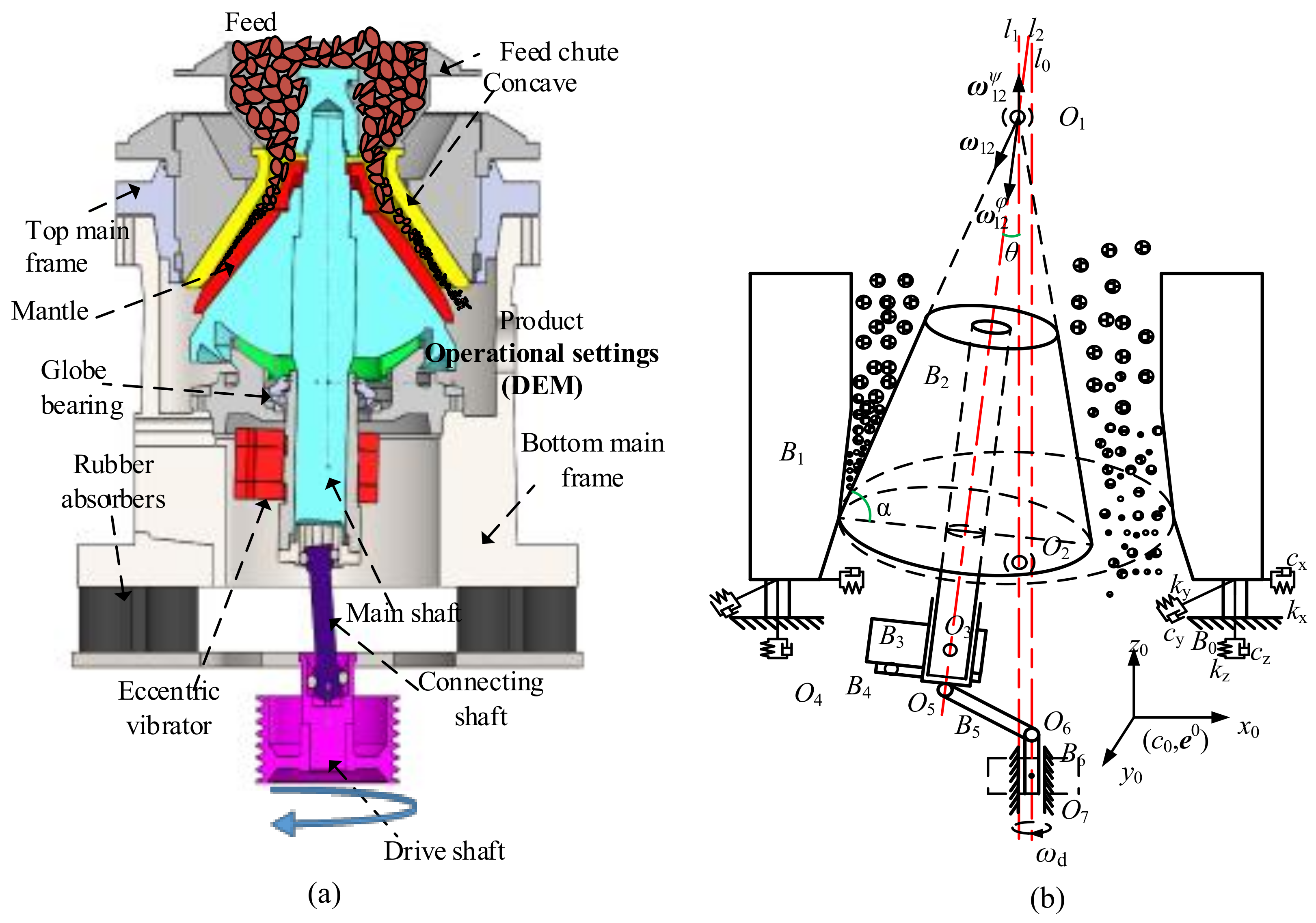
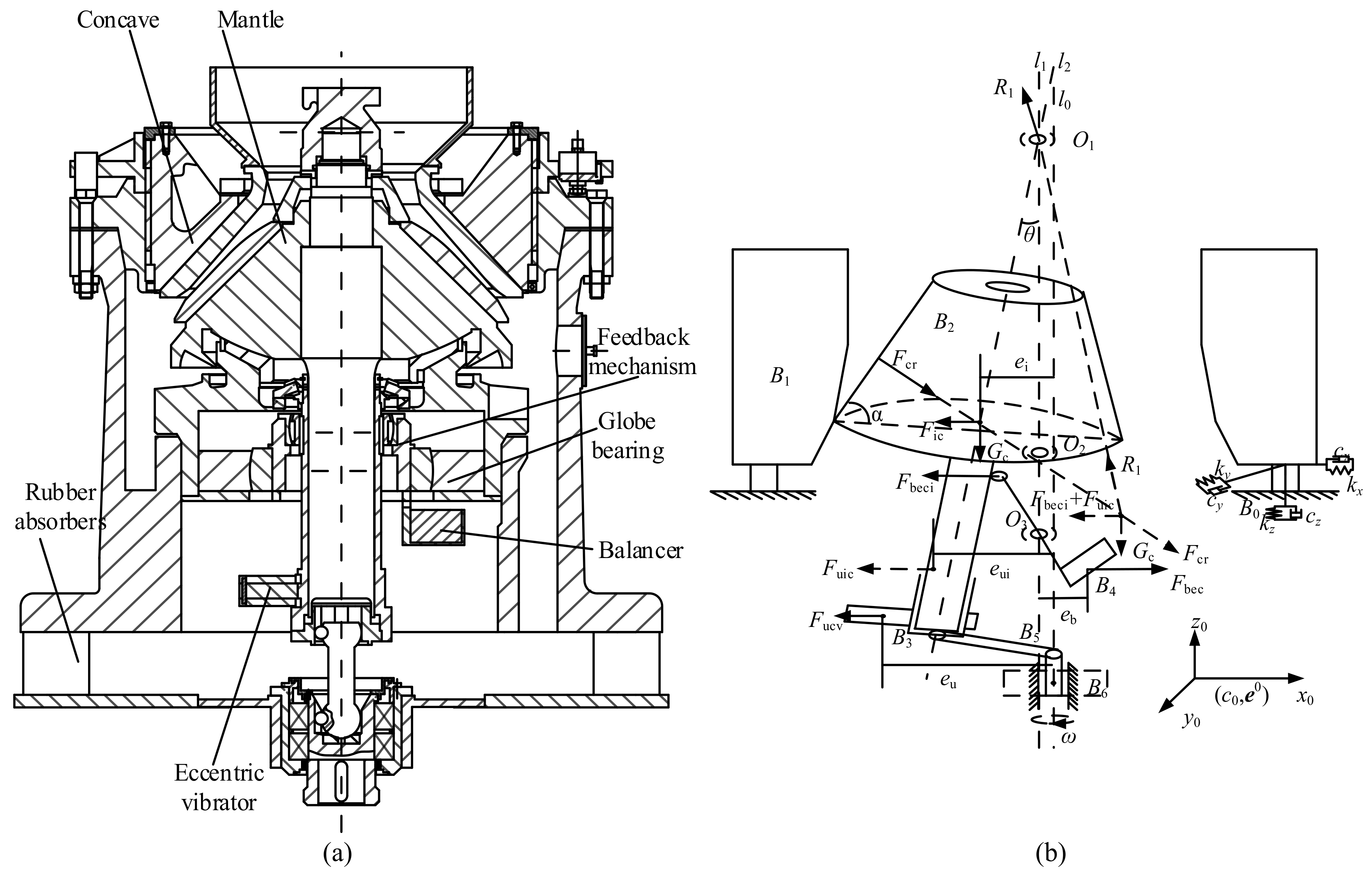
2.1. Inertia Cone Crusher Theory

The inertia cone crusher consists of a main frame, a concave, a mantle, rubber absorbers, a main shaft and an eccentric vibrator. The ore particles fall from the feed chute to the crushing chamber; then, they are squeezed by the mantle and other particles. Finally, the particles are discharged from the discharge zone. Figure 1 shows a vertical cross-section and a simplified MBD model for an inertia cone crusher, where α and θ are the mantle angle and the nutation angle, respectively. l₀, l₁ and l₂ are the axis of the crusher, concave and mantle, respectively. B₁ is the fixed cone, which is fixed to the main frame. B₂ is the moving cone, which is fixed to the main shaft. O₁ is a spherical joint; O₂ is a spherical joint between B₁ and the globe bearing (B₄); O₃ is a cylindrical joint between B₂ and the eccentric vibrator (B₃); O₄ is a planar joint between B₃ and B₄; O₅ is a ball-pin joint between B₃ and the connecting shaft (B₅); O₆ is a universal joint between B₅ and the drive shaft (B₆); O₇ is a revolute joint between B₆ and the ground (B₀).

2.2. Crusher Dynamic Model Using MBD

The generalized coordinate q_i of the rigid body B_i is shown in Equation (1).

$$q_i={\left(r_i{}^{\mathrm{T}},{\Lambda }_i{}^{\mathrm{T}}\right)}^{\mathrm{T}}={\left(x_i, y_i, z_i, {\psi }_i, {\theta }_i, {\phi }_i\right)}^{\mathrm{T}}, i=1,.....,6$$

(1)

where r_i is the matrix of independent position variables (x_i, y_i, z_i), and Λ_i is the matrix of independent angle variables (ψ_i, θ_i, φ_i). According to [18], the kinetic formula for B_i without any joint equations is derived in Equation (2).

$$M_i{\ddot{q}}_i=Q_i$$

(2)

where ${\ddot{q}}_i$ is the generalized acceleration of q_i, and M_i and Q_i can be expressed, respectively:

$$M_i=\left[\begin{array}{cc}{m}_i{E}_{3\times 3}& 0_{3\times 3}\\ 0_{3\times 3}& J_i^{(i)}{D}_i\end{array}\right], Q_i=\left[\begin{array}{c}{F}_{ia}+F_{if}+F_{ig}+F_{ic}+F_{ip}\\ -\left(J_i^{(i)}{\dot{D}}_i+\left(D_i\dot{\Lambda }\right)J_i^{(i)}{D}_i\right){\dot{\Lambda }}_i+T_{ia}^{(i)}+T_{if}^{(i)}+T_{ic}^{(i)}+T_{ip}^{(i)}\end{array}\right]$$

(3)

where m_i and J_i are the mass and the inertia matrix for B_i, respectively. E and 0 denote the identity and null matrix, respectively. F_ia and T_ia denote the equivalent absorber forces and torques, F_if and T_if denote the joint friction forces and torques, F_ig is the gravity of B_i, F_ip and T_ip denote the equivalent particle forces and torques, and D_i is the coordinate matrix.

The formula of MBD for the inertia cone crusher without any joints can be shown as:

$$\left\{\begin{array}{c}M\ddot{q}=Q\\ M=\mathrm{diag}(M_1, M_2, M_3, M_4, M_5, M_6)\\ Q={(Q_1^{\mathrm{T}}, Q_2^{\mathrm{T}}, Q_3^{\mathrm{T}}, Q_4^{\mathrm{T}}, Q_5^{\mathrm{T}}, Q_6^{\mathrm{T}})}^{\mathrm{T}}\end{array}\right.$$

(4)

where $\ddot{q}$ is the generalized accelerations of the multi-body system. The joint O_j (j = 1,2,…,7) equations and driving motion constraints for inertia cone crusher are expressed as:

$$\Phi (q,t)=0, {\Phi }_q=\frac{\partial \Phi }{\partial q}=\left[\frac{\partial {\Phi }_i}{\partial q_j}\right] ; i=1,.....,26, j=1,.....,7$$

(5)

According to Equation (5), the velocity and acceleration equation can be expressed as:

$$\left\{\begin{array}{c}{\Phi }_q\dot{q}=-{\Phi }_t\\ {\Phi }_q\ddot{q}=\zeta \end{array}\right., \zeta =-\left[{\left({\Phi }_q\dot{q}\right)}_q\dot{q}+2{\Phi }_{qt}\dot{q}+{\Phi }_{tt}\right]$$

(6)

whereΦ_q and Φ_t is the Jacobian matrix for Φ(q,t). According to the Lagrange multiplier λ_i (i = 1, 2, …, 26), the formula of MBD for inertia cone crusher is derived in terms of the Lagrange multiplier matrix λ and generalized coordinate matrix q, and can be shown as:

$$\left[\begin{array}{cc}M& {\Phi }_q^{\mathrm{T}}\\ {\Phi }_q& 0\end{array}\right]\left[\begin{array}{c}\ddot{q}\\ \lambda \end{array}\right]=\left[\begin{array}{c}Q\\ \zeta \end{array}\right], \lambda ={\left({\lambda }_1, {\lambda }_2, \cdots , {\lambda }_{26}\right)}^{\mathrm{T}}$$

(7)

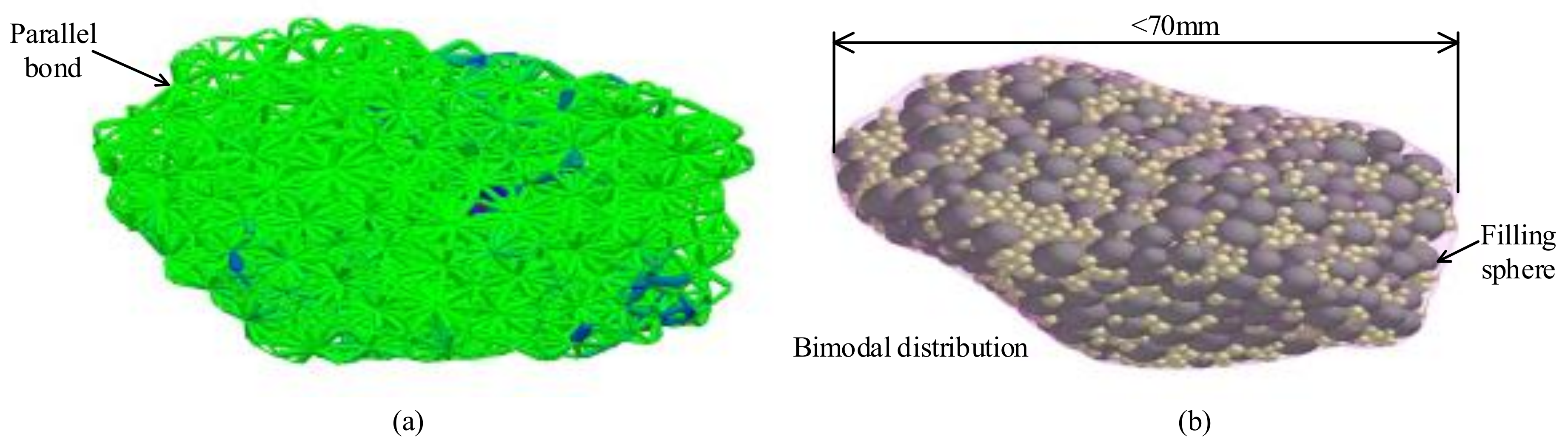
2.3. DEM Modeling of Slag Particles Using BPM

2.3.1. BPM Theory

The BPM consists of bonding a packed distribution of particles, forming a breakage cluster [19]. As shown in Figure 2, a parallel bonding beam is created between each particle in contact, so the forces (torques) on the bonding beam are calculated from Equation (8) and Equation (9). BPM has been used in simulating the crushing behavior of particles [13,20,21].

$$\delta F_{bn}=-k_{bn}A\Delta U_n, \delta F_{bt}=-k_{bt}A\Delta U_t, \delta T_{bn}=-k_{bn}J\Delta {\Theta }_n, \delta T_{bt}=-k_{bt}\frac{J}{2}\Delta {\Theta }_t$$

(8)

where F_bn, T_bn, F_bt and T_bt denote the bond normal force, normal torque, bond tangential-directed force and torque, respectively. k_bn and k_bt are the normal and tangential stiffness per unit area. A and J are the area of the parallel bond cross-section and polar moment of inertia, respectively.

$$\Delta U_n=v_n\delta t , \Delta U_t=v_t\delta t, A=\mathsf{\pi }{R}_b^2, \Delta {\Theta }_n={\omega }_n\delta t, \Delta {\Theta }_t={\omega }_t\delta t, J=\frac{1}{2}\mathsf{\pi }{R}_b^4$$

(9)

where R_b, V_n, V_t, ω_n, ω_t, and δt are parallel bond radius, normal velocity, tangential velocity, normal angular velocity, tangential angular velocity and time step, respectively.

The maximum normal and tangential stress are calculated according to Equation (10).

$${\sigma }_b^{\max }={\left|\frac{\left|F_{bn}\right|}{A}+\frac{2\left|T_{bt}\right|}{J}{R}_b\right|}_{\max }<{\sigma }_{bc},{\tau }_b^{\max }={\left|\frac{\left|F_{bt}\right|}{A}+\frac{\left|T_{bn}\right|}{J}{R}_b\right|}_{\max }<{\tau }_{bc}$$

(10)

where σ_bc and τ_bc are critical normal and critical shear strength, respectively. If the maximum stress exceeds the critical strength, the bond beam will disappear. The particle interaction depends on the Hertz–Mindlin contact model [22].

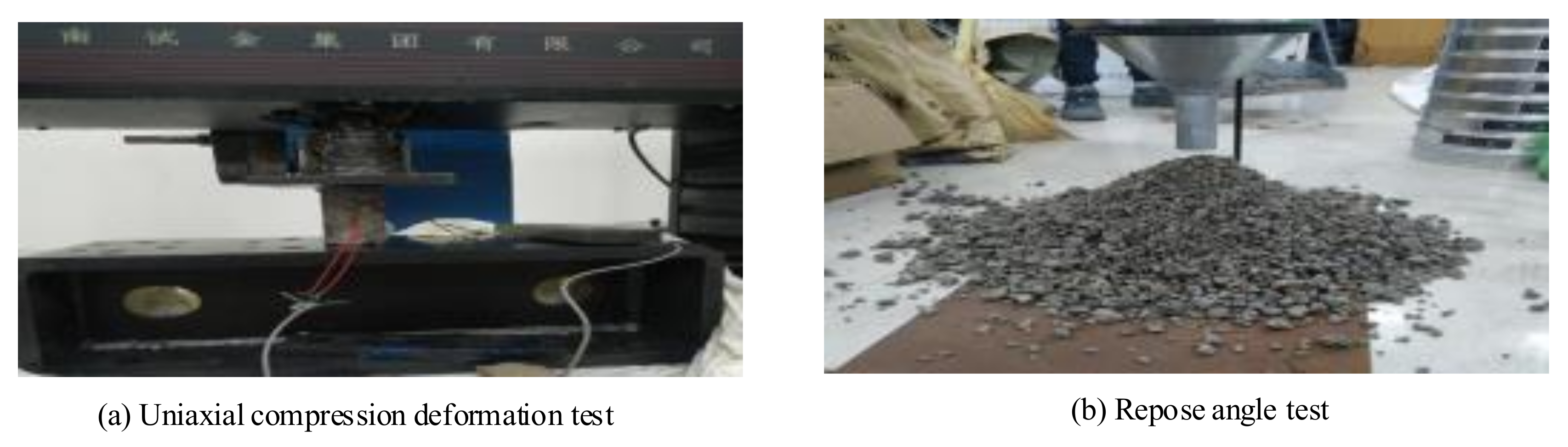
2.3.2. BPM Calibration

The feed material is a steel slag which has a complex shape and size distribution in our industrial experiments of the inertia cone crusher. The feed particle size range is 50 mm to 70 mm, and a 3D model of slag is shown in Figure 3. When using BPM for simulating the crushing behavior of steel slag, the key is to make sure that the relevant DEM parameters of the particle are calibrated. Therefore, the Hertz–Mindlin contact model parameters were determined by the uniaxial compression deformation and repose angle test, as shown in Figure 4.

Table 1. Simulation parameters for MBD–DEM.

Parameter	Value		Unit
DEM material properties
	Rock	Steel
Solid density	4700	7800	(kg/m3)
Shear stiffness	1.48∙109	7.0∙1010	(Pa)
Poisson’s ratio	0.38	0.3
	Rock_Rock	Rock_Steel
Coefficient of static friction	0.56	0.7
Coefficient of restitution	0.15	0.25
Coefficient of rolling friction	0.01	0.01
BPM parameters
Normal stiffness	556		(GPa/m)
Shear stiffness	250		(GPa/m)
Normal critical stress	32		(MPa)
Shear critical stress	8.5		(MPa)
Bond disc radius	3.2		(mm)
Machine
Mantle cone angle	50		(deg)
Driving speed	550		(rpm)
Fixed cone mass	20,000		(kg)
Moving cone mass	5500		(kg)
Rubber absorber properties
Stiffness coefficient kx,ky,kz	350,350,970		(N/mm)
Damping coefficient cx,cy,cz	20,20,40		(N·s/mm)

shows the contact parameters.

The BPM-relevant parameters were determined by the Brazilian test and simulation experiment, as shown in Figure 5. The calibration method had been described in detail in our publication [13]. By comparing the tensile strength simulation with the experiment values (10.6 MPa), we directly provide the BPM parameters that are shown in Table 1.

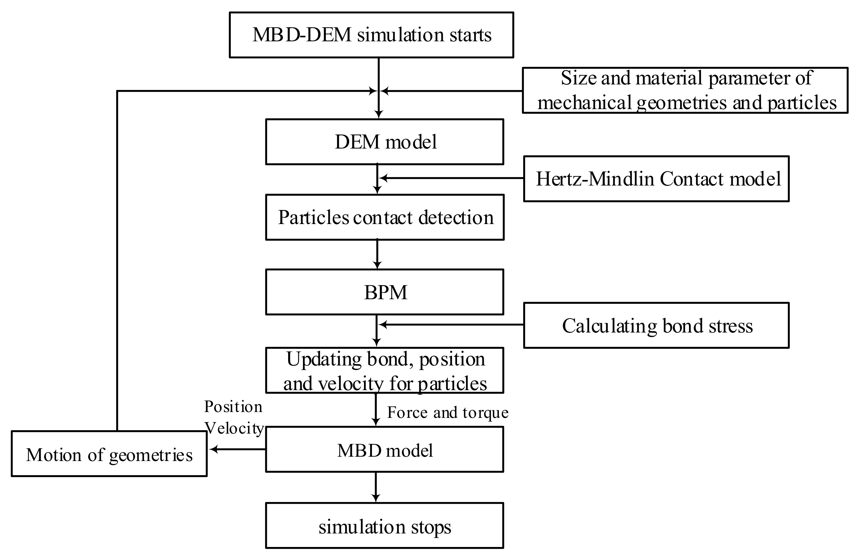
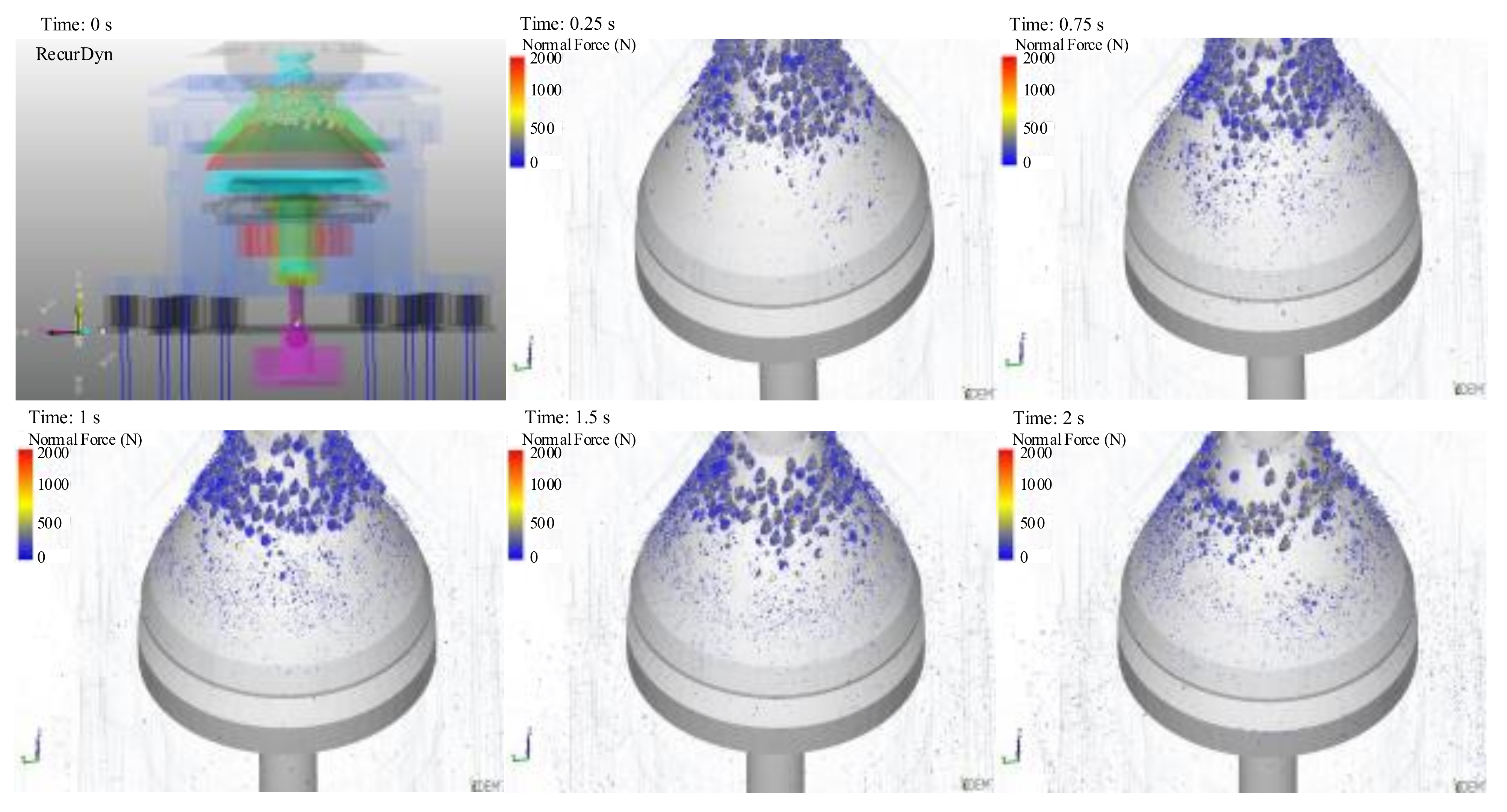
2.4. The Solution of the Coupled MBD-DEM Model in Software

Combining with Section 2.1, Section 2.2 and Section 2.3, Figure 6 shows the simulation flowchart of the inertia cone crusher using the MBD–DEM coupling method. The MBD of the geometries is calculated by RecurDyn software, and the DEM of the particles is calculated using EDEM. As slag clusters flow downward between the mantle and the concave, the size becomes successively smaller in the software EDEM, as shown in Figure 7. The operative performances (the operative crushing force, amplitude and average power) for the inertia cone crusher are obtained by the software RecurDyn.

3. Analysis of the Inertia Cone Crusher Performance

3.1. Influencing Factors and Performance Goals

Basing on Section 2 and the previous publications [3,4,5], the fixed cone mass (FM) m₁ and the moving cone mass (MM) m₂ are taken as the influencing factors. The operative crushing force F_o is less than the theoretical crushing force F_t under normal operating conditions. The theoretical crushing force of the inertia cone crusher is provided by the moving cone when the fixed cone is not moving. As such, the crushing force achievement rate η_f is taken as one of the performance goals, according to Equation (11).

$${\eta }_{\mathrm{f}}=100\%\times F_{\mathrm{o}}/F_{\mathrm{t}}$$

(11)

when the inertia cone crusher works, the fixed cone will move horizontally and deflect around a rotation point. As such, the amplitude of the rotation point displacement and the deflection angle can give a good indication for the vibration characteristics of the crusher. The theoretical and experimental results indicate that the amplitude A_s and deflection angle γ_d have a significant positive correlation [22,23]. Ignoring the deflection angle γ_d, the amplitude A_s is taken as a performance goal. Besides this, the two mass variables have a great impact on the energy consumption of a crusher, and the average power draw of drive shaft P_a is taken as a performance goal. Based on the response surface methodology (RSM) [24], the influence of the two mass variables on the performance goals is modeled with the SPSS software. The corresponding predictive regression models can be expressed as Equation (12), and the simulated experiment scheme is listed in Appendix A,

Table A1. Simulated experiment scheme of two mass variables.

Simulation Run	FM—m1 (t)	MM—m2 (t)	Achievement Rate—ηf (%)	Operative Force—Fo (kN)	Amplitude—As (mm)	Deflection Angle—γd (deg)	Average Power—Pa (kW)
1	11	3.1	85.79	418.43	7.09	0.213	105.39
2	11	3.5	82.96	455.65	7.85	0.239	118.06
3	11	4.0	81.97	515.24	8.75	0.269	154.19
4	11	4.5	80.04	562.98	9.63	0.301	171.62
5	11	5.0	79.38	623.81	10.59	0.329	199.30
6	11	5.5	75.76	653.85	11.36	0.358	231.51
7	11	5.9	73.83	697.79	11.95	0.383	248.23
8	15	3.1	88.75	432.20	6.31	0.177	86.16
9	15	3.5	86.36	472.11	7.03	0.198	100.78
10	15	4.0	85.34	536.38	7.78	0.225	133.59
11	15	4.5	84.35	593.22	8.64	0.254	148.01
12	15	5.0	81.94	643.82	9.39	0.280	168.72
13	15	5.5	78.48	666.15	10.16	0.304	207.90
14	15	5.9	77.67	723.95	10.77	0.326	229.78
15	20	3.1	90.87	443.19	5.23	0.145	79.47
16	20	3.5	89.18	491.92	5.86	0.164	88.69
17	20	4.0	88.13	553.81	6.55	0.186	121.53
18	20	4.5	87.67	616.62	7.22	0.213	135.34
19	20	5.0	85.67	673.25	7.91	0.231	149.18
20	20	5.5	81.87	697.92	8.41	0.254	187.17
21	20	5.9	80.71	743.23	9.08	0.272	202.72
22	25	3.1	92.94	452.84	4.21	0.121	73.14
23	25	3.5	91.15	502.39	4.76	0.135	76.02
24	25	4.0	90.29	570.54	5.32	0.155	105.89
25	25	4.5	89.87	643.46	5.99	0.176	122.67
26	25	5.0	88.31	694.31	6.45	0.193	138.81
27	25	5.5	84.91	726.74	7.05	0.231	165.17
28	25	5.9	87.01	779.00	7.48	0.229	184.56
29	30	3.1	94.36	459.72	3.47	0.102	68.53
30	30	3.5	92.97	510.62	3.91	0.115	72.56
31	30	4.0	92.12	578.33	4.40	0.131	93.88
32	30	4.5	91.48	645.52	4.81	0.149	113.45
33	30	5.0	89.96	706.50	5.35	0.163	129.62
34	30	5.5	87.39	754.20	5.83	0.180	149.31
35	30	5.9	86.84	799.67	6.21	0.193	155.07
36	35	3.1	95.48	465.18	2.83	0.087	64.54
37	35	3.5	93.80	515.13	3.08	0.094	69.68
38	35	4.0	92.91	585.44	3.59	0.113	82.87
39	35	4.5	92.96	653.76	3.98	0.128	109.54
40	35	5.0	91.02	716.72	4.46	0.141	121.50
41	35	5.5	91.04	785.69	4.66	0.155	134.31
42	35	5.9	89.98	827.12	4.91	0.168	136.34
43	39	3.1	96.68	470.81	2.47	0.079	62.20
44	39	3.5	94.36	520.17	2.77	0.880	67.96
45	39	4.0	94.13	591.51	3.09	0.100	78.30
46	39	4.5	93.44	657.93	3.39	0.114	105.51
47	39	5.0	92.38	725.88	3.77	0.125	114.60
48	39	5.5	92.08	802.48	3.91	0.138	128.06
49	39	5.9	90.88	836.75	4.43	0.149	129.78

.

$$\left\{\begin{array}{c}{\eta }_{\mathrm{f}}=f_{\eta }(m_1,m_2)\\ A_{\mathrm{s}}=f_A(m_1,m_2)\\ P_{\mathrm{a}}=f_P(m_1,m_2)\end{array}\right.;\begin{array}{c}10\le m_1\le 45\\ 3\le m_2\le 6.5\end{array}$$

(12)

where f_η, f_A, and f_P are the predictive models of crushing force achievement rate, amplitude and average power, respectively. Because the driving speed is determined by the productivity, the driving speed of the crusher (model: GYP1200) should not exceed 550 rpm. As such, the driving speed is set to 550 rpm in this paper.

3.2. Crushing Force Achievement Rate Analysis

The influence of FM and MM on the crushing force achievement rate, and the prediction regression curves are shown in Figure 8. The theoretical force F_t is only determined by MM, and Figure 8a shows the influence of MM on the theoretical force F_t. Figure 8b shows the influence of FM on the crushing force achievement rate under three kinds of MM (3.5 t, 4.5 t, and 5.9 t), which indicates that the crushing force achievement rate η_f increases significantly with increasing FM. Figure 8c shows the influence of MM on η_f under three kinds of FM (15 t, 25 t, and 39 t), which indicates that η_f gradually decreases with increasing MM. At the 0.05 significance level, we can find that the influence of FM and MM on η_f is significant using the quadratic regression function.

Figure 8d shows the influence of the interaction between FM and MM on η_f using the response surface methodology (RSM), and the corresponding results of ANOVA for predictive regression models are shown in

Table 2. The results of ANOVA for predictive regression model.

Model		Degree Freedom	Mean Square	F Value	p Value	Determination Coefficient
fη	Regression	4	363.167	767.995	<0.01	0.993
	Error	44	0.473
	Total	48
fA	Regression	4	75.010	9625.911	<0.01	0.999
	Error	44	0.008
	Total	48
fP	Regression	4	27,049.462	954.059	<0.01	0.989
	Error	44	28.352
	Total	48

. The prediction regression model of the crushing force achievement rate is expressed as:

$${\eta }_{\mathrm{f}}=f_{\eta }(m_1,m_2)=82.196+0.628m_1-0.011m_1^2-0.557m_2^2+0.083m_1{m}_2; 10\le m_1\le 45, 3\le m_2\le 6.5$$

(13)

The corresponding ANOVA for predictive regression coefficients is shown in

Table A2. The results of ANOVA for prediction regression coefficients.

Model		Regression Coefficient—B	Standardization Coefficient—Be	t Value	p Value	Confidence Interval for B
						Lower	Upper
fη	FM	0.628	1.097	7.718	<0.01	0.464	0.792
	MM		−0.400	−1.943	0.59
	FM·FM	−0.011	−0.937	−8.080	<0.01	−0.013	−0.08
	MM·MM	−0.557	−0.878	−17.980	<0.01	−0.619	−0.494
	FM·MM	0.083	0.759	7.940	<0.01	0.062	0.104
	Constant	82.196		82.400	<0.01	80.185	84.206
fA	FM	−0.197	−0.762	−18.703	<0.01	−0.225	−0.169
	MM	2.162	0.836	58.740	<0.01	2.063	2.261
	FM·FM	0.003	0.583	17.664	<0.01	0.0025	0.0034
	MM·MM		−0.131	−2.331	0.025
	FM·MM	−0.039	−0.799	−28.692	<0.01	−0.043	−0.036
	Constant	3.708		19.341	<0.01	3.192	4.224
fP	FM	−1.679	−0.340	−2.641	0.011	−2.960	−0.398
	MM	64.107	1.299	28.872	<0.01	59.632	68.582
	FM·FM	0.068	0.697	6.689	<0.01	0.048	0.088
	MM·MM		0.174	0.935	0.355
	FM·MM	−0.979	−1.039	−11.804	<0.01	−1.146	−0.812
	Constant	−56.084		−4.850	<0.01	−79.391	−32.777

. At the 0.05 significance level, we can find that the linear term of MM has the weakest impact on η_f, and the p-value is more than 0.05. As such, the linear term of MM is ignored in the prediction regression model of crushing force achievement rate. As FM increases or MM decreases, η_f can increase. This is because the increase in FM or the decreases in MM will decrease the amplitude of the fixed cone, and increase the eccentric distance of the moving cone. However, when η_f is over 90%, the increase in η_f is very small with increasing FM, and for the different moving cone mass, the fixed cone mass required to reach 90% (η_f) is different.

3.3. Amplitude Analysis

The influence of FM and MM on the amplitude of the fixed cone, and the prediction regression curves, are shown in Figure 9. Figure 9a shows the influence of FM on the amplitude under three kinds of MM (3.5 t, 4.5 t, and 5.9 t), which indicates that the amplitude A_s decreases with increasing FM. Figure 9b shows the influence of MM on the amplitude under three kinds of FW (15 t, 25 t, and 39 t), which indicates that the amplitude A_s increases with increasing MM. Figure 9c shows the influence of the interaction between FM and MM on the crushing force achievement rate η_f using RSM, and

Table 3. The summary of experimental averaged results.

Experiment Case		Amplitude of First Point (mm)	Amplitude of Second Point (mm)	Amplitude of Rotation Point (mm)	Deflection Angle (mm)
450 rpm	Balance	0.18	0.55	0.04	0.18
	Without	0.49	2.11	0.22	0.63
650 rpm	Balance	0.21	0.66	0.05	0.24
	Without	0.55	2.47	0.25	0.67

indicates that the prediction model of A_s has a good fitness using the quadratic regression function with the 0.01 significance level. The prediction regression model is shown in Equation (14).

$$A_{\mathrm{s}}=f_A(m_1,m_2)=3.708+2.162m_2-0.197m_1+0.003m_1^2-0.039m_1{m}_2; 10\le m_1\le 45, 3\le m_2\le 6.5$$

(14)

It can be found that the quadratic term of MM has the weakest impact on amplitude, and the p-value is more than 0.01 from Table A2. So, the quadratic term of MM is ignored in the predictive regression model of amplitude. As FM increases, the amplitude A_s can decrease, and the fixed cone will be more difficult to move for a constant theoretical crushing force. Comparing Figure 8d and Figure 9c, it can be found that when the η_f is over 90%, the decrease in amplitude A_s is very small with the increasing FM. However, with the change of MM, the amplitude A_s will change significantly for a constant FM.

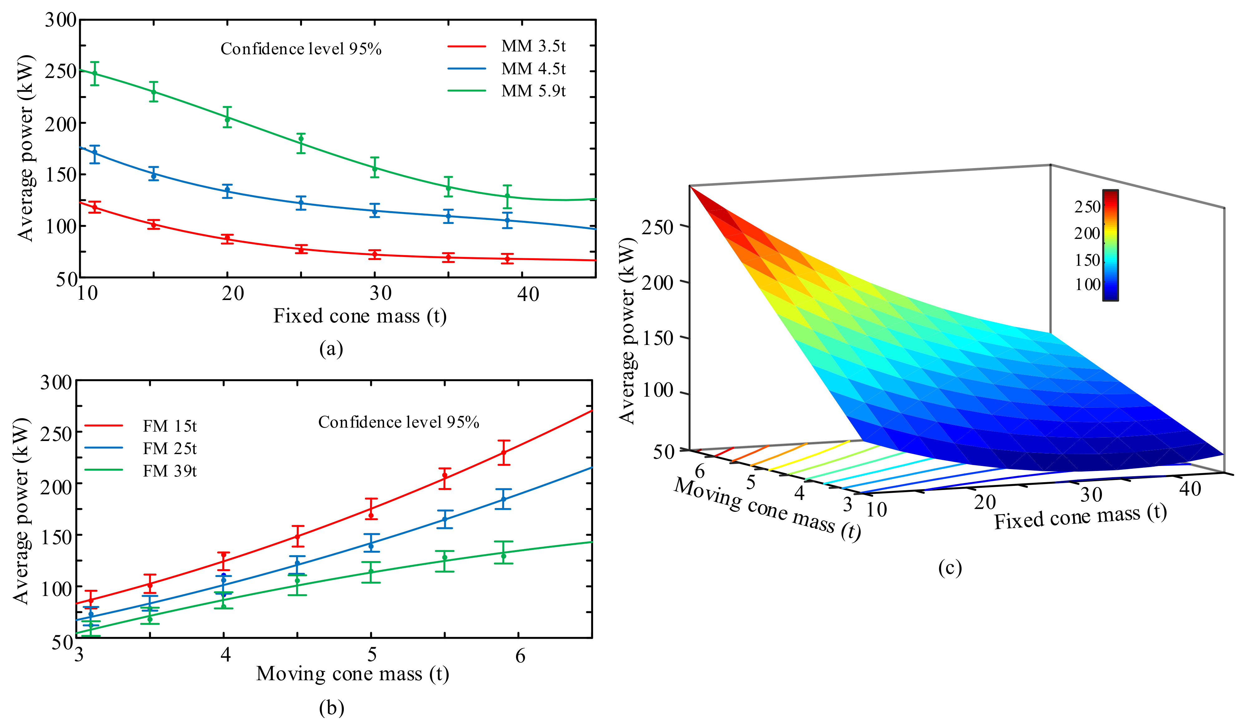
3.4. Average Power Analysis

The influence of FM and MM on the average power draw, and the prediction regression curves, are shown in Figure 10. Figure 10a shows the influence of FM on the average power under three kinds of MM (3.5 t, 4.5 t, and 5.9 t), which indicates that the average power P_a decreases with increasing FM. Figure 10b shows the influence of MM on P_a under three kinds of FM (15 t, 25 t, and 39 t), which indicates that the average power P_a increases significantly with increasing MM. Figure 10c shows the influence of the interaction between FM and MM on P_a using RSM, and Table 3 indicates that the prediction model of average power P_a has a good fitness using the quadratic regression function with the 0.05 significance level. The prediction regression model is shown in Equation (15). Table A2 shows that the quadratic term of MM has the weakest impact on the average power P_a, and the p-value is more than 0.05.

$$A_{\mathrm{s}}=f_A(m_1,m_2)=-56.084+64.107m_2-1.679m_1+0.068m_1^2-0.979m_1{m}_2; 10\le m_1\le 45, 3\le m_2\le 6.5$$

(15)

Comparing Figure 9 and Figure 10, we can see that as FM and MM increase, the variation in average power P_a is similar to that of the amplitude A_s. The reason for this is that as A_s increases, the energy consumption of the rubber absorbers can increase, and the kinetic energy of the steel slag particles also increases, resulting in the increase in friction heat energy.

3.5. Optimization Results

Combining with the above sections, it can be seen that when the crushing force achievement rate η_f is over 90%, the decrease in amplitude A_s and average power P_a are very small with increasing FM. Table 1 shows the FM is 20 t and the MM is 5.5 t for the industrial inertia cone crusher (model: GYP1200), and the operative crushing force F_o is 697.92 kN from the simulated experiment (Table A1). If the prediction values of F_o and η_f are 697.92 kN and 90%, the MM is set to 4.95 t (Figure 8a). According to Equation (13), the optimized fixed cone mass is 30.54 t.

According to Equations (14) and (15), the optimized amplitude A_s and average power P_a are 5.29 mm and 125.38 kW, respectively. Compared with the simulated experiment (Table A1), it can be seen that the optimized amplitude, average power and MM are decreased by 37.1%, 33.1% and 10.2%, respectively. Finally, we can see that the decrease in amplitude can effectively decrease the average power, and increase the crushing force achievement rate. However, the optimized FM is increased by 52.7%, so the optimized mass of the inertia cone crusher is about three times as much as the hydraulic cone crusher or spring crusher for the same industrial scale, which increases the manufacturing cost. In this paper, we design a more effective dynamic balancing mechanism for the inertia cone crusher, which decreases the amplitude and minimizes the mass of the inertia cone crusher.

4. Design of Dynamic Balancing Mechanism

4.1. Mechanics Principle of Dynamic Balancing

The total crushing force of the single exciter GYP-type inertia cone crusher is provided by the eccentric vibrator and the mantle, as shown in Equation (16):

$$F_{\mathrm{cr}}=F_{\mathrm{ice}}+F_{\mathrm{ucve}}$$

(16)

where F_cr is the total crushing force, F_ice is the equivalent centrifugal force generated by the mantle, and F_ucve is the equivalent exciting force generated by the eccentric vibrator.

The inertia cone crusher with the dynamic balancing mechanism is shown in Figure 11a. The dynamic balancing mechanism is mainly composed of a balancer and feedback mechanism. A balancer is added to the GYP-type inertia cone crusher, which can similarly rotate on the opposite side of the vibration exciter. In this way, the vibration of the crusher can be minimized to decrease the mass of the fixed and moving cone. Through a feedback mechanism to increase the crushing force, the kinetic energy of the balancer can be utilized efficiently.

The planar layout of forces acting on the mantle cone is shown in Figure 11b. F_ic, F_ucv and F_bec are the centrifugal forces generated by the mantle, eccentric vibrator and balancer, respectively.

$$F_{\mathrm{ic}}=m_{\mathrm{ic}}{\omega }^2{e}_{\mathrm{i}}; F_{\mathrm{ucv}}=m_{\mathrm{ucv}}{\omega }^2{e}_{\mathrm{u}}; F_{\mathrm{bec}}=m_{\mathrm{bec}}{\omega }^2{e}_{\mathrm{b}}$$

(17)

where m_ic, m_ucv and m_bec are the mass of the mantle, eccentric vibrator and balancer, respectively; e_ic, e_ucv and e_bec are the eccentric distance of the mantle, eccentric vibrator and balancer, respectively; ω is the drive shaft speed. The value of F_bec should conform to Equation (18).

$$F_{\mathrm{uic}}=\left(m_{\mathrm{ucv}}+m_{\mathrm{ic}}\right){\omega }^2{e}_{\mathrm{ui}}=F_{\mathrm{bec}}$$

(18)

where F_uic is the equivalent force of the centrifugal force generated by the moving cone, and e_ui is the equivalent eccentric distance of the moving cone. Based on the lever principle, the vector force F_beci can be expressed as

$$F_{\mathrm{cr}}+F_{\mathrm{beci}}+F_{\mathrm{uic}}+R_1+G_{\mathrm{c}}=0$$

(19)

where F_beci is the force acting on the moving cone by the feedback mechanism, R₁ is the constraint reaction of spherical joint O₁, and G_c is the gravity of the moving cone.

Compared with Equations (16) and (19), it can be seen that the inertia cone crusher with the dynamic balancing mechanism adds the feedback force compared with the single exciter crusher. Therefore, the dynamic balancing mechanism can obviously decrease the amplitude of the fixed cone and increase the crushing force. In this way, the mass of the fixed and moving cone is minimized, and the manufacturing cost decreases significantly.

4.2. Elementary Prototype of Laboratory Experiments

4.2.1. Experimental Devices

Corresponding experiments are validated to verify the dynamic balancing mechanism. However, it is an impossible task for us to manufacture an industrial-scale inertia cone crusher with the dynamic balancing mechanism. In this paper, a laboratory prototype with the same dynamic balancing mechanism is developed. The amplitude, power draw and product size distribution of the laboratory crusher can be collected by some experimental devices, and the results are compared with the crusher without the dynamic balancing mechanism. The crusher without the dynamic balance can provide the same theoretical crushing force as the dynamic balance prototype. The experimental devices and dynamic signal acquisition systems are shown in Figure 12. The feed material is a 7.5–10 mm white marble, and the amplitude, power draw and product size distribution for the two driving speed levels (450 and 650 rpm) are compared in the following sections.

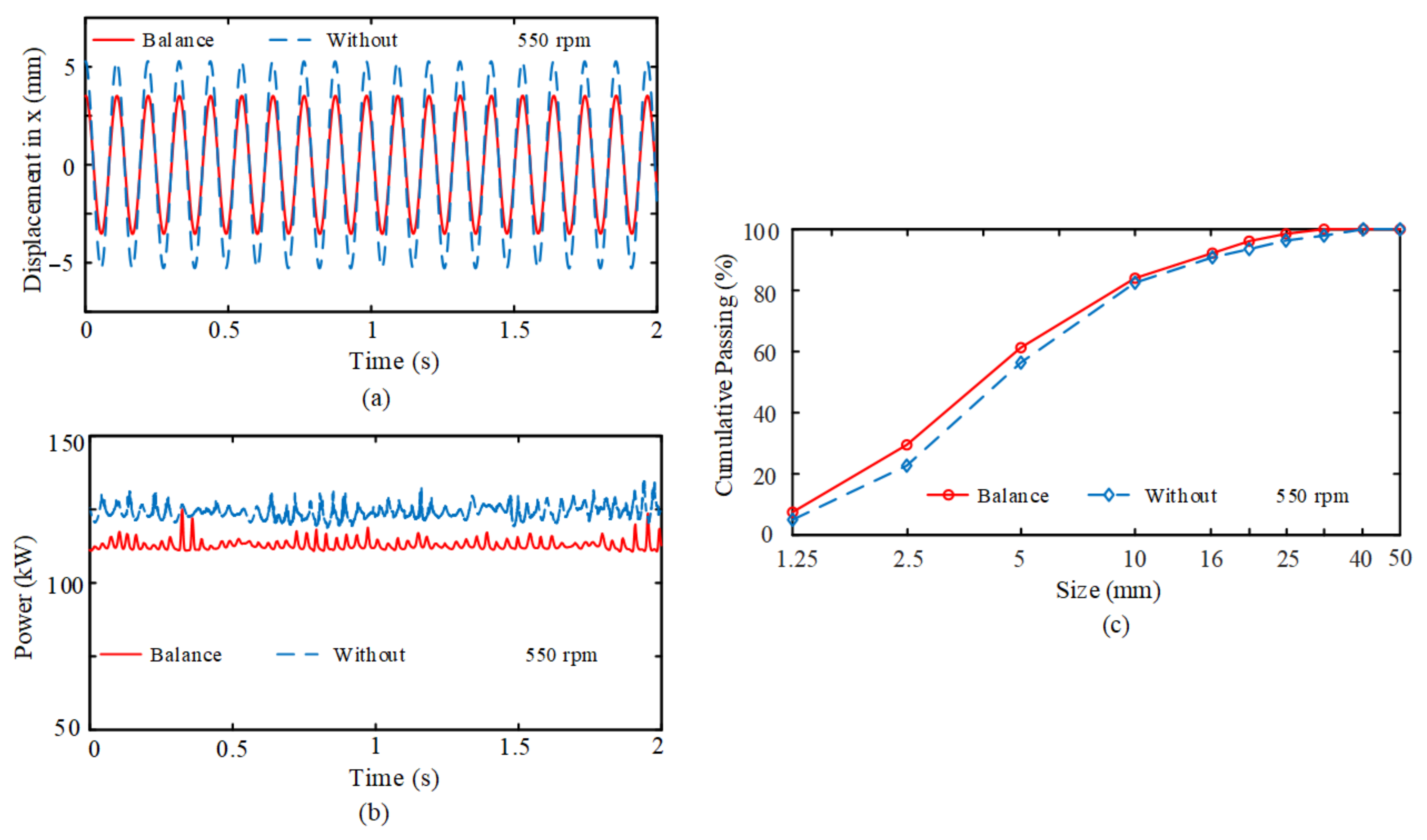
4.2.2. Amplitudes of Test Points

The displacements of two test point are sampled by displacement sensors in Figure 12a. The experimental data of two test points in the x direction are displayed for the drive speeds of 450 rpm and 650 rpm, as shown in Figure 13. In Table 3, the test data from the balancing crusher and without balancing mechanism are summarized. The results show that the amplitude and deflection angle of the balancing crusher are decreased by 80.6% and 64.2%, compared with the crusher without a balancing mechanism. Therefore, the good vibration reduction performance of the dynamic balancing mechanism is verified by experimental comparison.

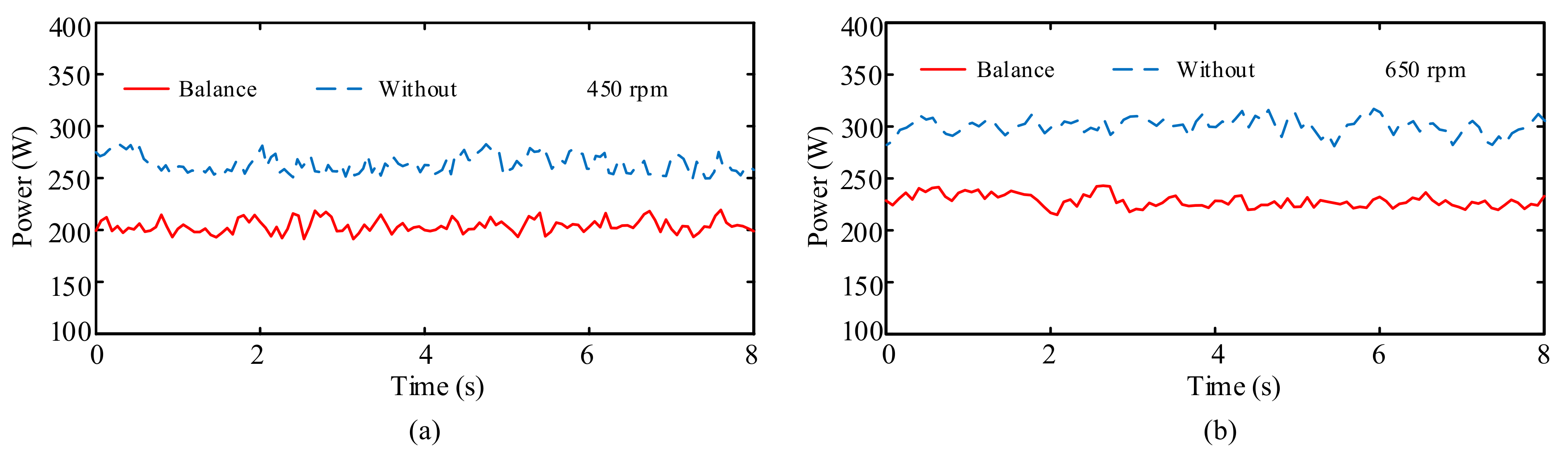
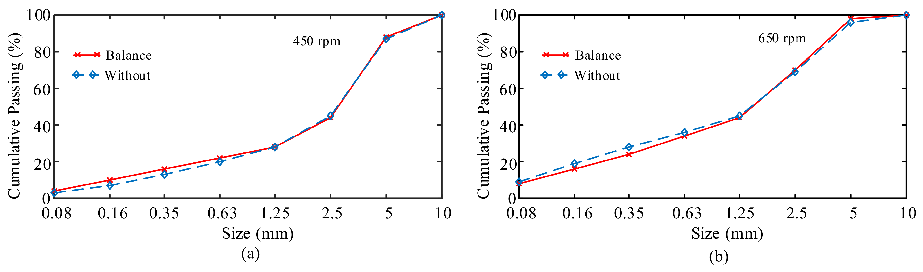
4.2.3. Power draw and Product Size Distribution

The input power of the motor is sampled by an electrical parameter test instrument in Figure 12b. The experimental data are displayed for the drive speeds of 450 rpm and 650 rpm, as shown in Figure 14. Figure 14 shows that the average power of the balancing crusher is decreased by 20.9%, compared with the crusher without a balancing mechanism. Therefore, the dynamic balancing mechanism can effectively reduce the energy consumption and running cost of the inertia cone crusher.

The product size distribution is collected by square sieves in Figure 12c. The experimental data are displayed for the drive speeds of 450 rpm and 650 rpm, as shown in Figure 15. The product size distribution displays a relatively good correspondence between the balancing mechanism and without the balance. It can be seen that the mechanism realizes the purpose of utilizing the inertia force and kinetic energy of the balancer.

4.3. Optimization Verification of Industrial-Scale Inertia Cone Crusher

To verify the optimization performances and two mass variables (FM and MM), the simulated experiments using MBD–DEM coupling are performed on the industrial-scale inertia cone crusher with the dynamic balancing mechanism. The fixed cone mass and the moving cone mass (including the dynamic balancing mechanism mass) are 6.44 t and 3.82 t, respectively. Compared with Section 3.4, the optimized crushing force achievement rate is over 95% using with the dynamic balancing mechanism. Furthermore, the optimized amplitude and average power are decreased by 33.1% and 10.2%, respectively, as shown in Figure 16.

In Figure 16c shows the product size distributions for the case balancing mechanism and the case without are compared. It can be seen that the balance case is slightly finer than the without-balance case. Due to the amplitude, the average power and product size distribution have been improved, and the good crushing performance of the dynamic balancing mechanism is verified in the industrial-scale inertia cone crusher. Furthermore, the fixed cone mass and the moving cone mass are decreased by 78.9% and 22.8%, respectively. The dynamic balancing mechanism significantly reduces the manufacturing cost.

5. Conclusions

In the inertia cone crusher design, an inevitable problem concerns how to determine the two mass variables (fixed cone mass and moving cone mass), which can affect the crusher dynamic performances. Firstly, the crushing process of the inertia cone crusher is simulated using the MBD–DEM coupling. Predictive regression models, in which the two mass variables are taken as influencing factors, and the crushing force achievement rate, amplitude and average power are taken as the performance goals, are explored by the design of simulation experiments. In addition, it is found that when the achievement rate η_f is over 90%, the decrease in amplitude A_s and average power P_a, and the increase in η_f, are very small with increasing FM. Due to the optimized values of η_f and FM being 90% and 30.54 t, the optimized amplitude A_s, average power P_a, and MM are decreased by 37.1%, 33.1% and 10.2%, respectively, compared with the original crusher.

The optimized FM is increased by 52.7%, which increases the manufacturing cost. In this paper, a new and more cost-effective dynamic balancing mechanism of inertia cone crusher is achieved in order to reduce FM. The vibration reduction and inertia force utilization of the dynamic balancing mechanism are verified by the elementary prototype of the laboratory experiment. Moreover, the effect of FM and MM reduction is verified by the MBD–DEM simulation of the industrial inertia cone crusher. Compared with the without-balance case (Section 3.4), the amplitude, average power and product size distribution have been improved, and the FM and MM are decreased by 78.9% and 22.8%. As such, from a manufacturer’s perspective, the manufacturing cost decreases significantly. In order to reduce the running costs for users, the future work will prioritize manually using the design of simulation experiments around the optimum drive shaft speed, the eccentric distance of eccentric vibrator and the discharge gap.

References

1. Safronov, A.N.; Kazakov, S.V.; Shishkin, Y.V. New trends in inertia cone crusher studies. Miner. Process. J. 2012, 5, 40–42. [Google Scholar]
2. Babaev, R.M.; Kishchenko, V.L. The effect of KID-1500 inertia cone crusher parameters upon preset crushed stone size fraction yield. Miner. Process. J. 2012, 1, 22–24. [Google Scholar]
3. Savov, S. Constructive-mechanical review of conical inertial crushers (KID). Bulg. J. Eng. Des. 2012, 15, 23–28. [Google Scholar]
4. Savov, S.; Nedyalkov, P.; Minin, I. Crushing force theoretical examination in one cone inertial crusher. J. Multidiscip. Eng. Sci. Technol. 2015, 2, 430–437. [Google Scholar]
5. Xia, X.; Chen, B. Study on dynamic characteristics of inertia cone crusher and its application. In Proceedings of the XXV International Mineral Processing Congress (IMPC 2010), Brisbane, Australia, 6–10 September 2010; pp. 1399–1403. [Google Scholar]
6. Cleary, P.W.; Sinnott, M.D.; Morrison, R.D.; Cummins, S.; Delaney, G.W. Analysis of cone crusher performance with changes in material properties and operating conditions using DEM. Miner. Eng. 2017, 100, 49–70. [Google Scholar] [CrossRef]
7. Andre, F.P.; Tavares, L.M. Simulating a laboratory-scale cone crusher in DEM using polyhedral particles. Powder Technol. 2020, 372, 362–371. [Google Scholar] [CrossRef]
8. Chen, Z.; Wang, G.; Xue, D.; Bi, Q. Simulation and optimization of gyratory crusher performance based on the discrete element method. Powder Technol. 2020, 376, 93–103. [Google Scholar] [CrossRef]
9. Cheng, J.; Ren, T.; Zhang, Z.; Liu, D.; Jin, X. A dynamic model of inertia cone crusher using the discrete element method and multi-body dynamics coupling. Minerals 2020, 10, 862. [Google Scholar] [CrossRef]
10. Xu, L. An approach for calculating the dynamic load of deep groove ball bearing joints in planar multibody systems. Nonlinear Dyn. 2012, 70, 2145–2161. [Google Scholar] [CrossRef]
11. Langerholc, M.; Cesnik, M.; Slavic, J.; Boltear, M. Experimental validation of a complex, large-scale, rigid-body mechanism. Eng. Struct. 2012, 36, 220–227. [Google Scholar] [CrossRef]
12. Li, C.; Honeyands, T.; O’Dea, D.; Moreno-Atanasio, R. The angle of repose and size segregation of iron ore granules: DEM analysis and experimental investigation. Powder Technol. 2017, 320, 257–272. [Google Scholar] [CrossRef]
13. Cundall, P.A.; Strack, O.D. A discrete numerical model for granular assemblies. Geotechnique 1979, 30, 331–336. [Google Scholar] [CrossRef] [Green Version]
14. Barrios, G.K.P.; Tavares, L.M. A preliminary model of high pressure roll grinding using the discrete element method and multi-body dynamics coupling. Int. J. Miner. Process. 2016, 156, 32–42. [Google Scholar] [CrossRef]
15. Chung, Y.C.; Wu, C.W.; Kuo, C.Y.; Hsiau, S.S. A rapid granular chute avalanche impinging on a small fixed obstacle: DEM modeling, experimental validation and exploration of granular stress. Appl. Math. Model. 2019, 74, 540–568. [Google Scholar] [CrossRef]
16. Znamenskll, S.B.; Krivelev, D.M. Inertial Cone Crusher for Comminution of Ores of Varying Hardness Has Base with Cylindrical Vertical Support Element, on Which Driving Counter-Balance Is Mounted on Bearings, Counter-Balance Including Concentric Portion with V Belt Groove. Russia Patent No. 2097132-C1, 20 February 1996. [Google Scholar]
17. Ren, T.; Huang, K.; Cheng, J.; Zhang, Z.; Jin, X. Vibration performance on novel inertia cone crushers. Chin. Mech. Eng. 2019, 30, 2704–2708. [Google Scholar]
18. Orin, D.E.; McGhee, R.B.; Vukobratovic, M.; Hartoch, G. Kinematic and kinetic analysis of open-chain linkages utilizing Newton-Euler methods. Math. Biosci. 1972, 43, 107–130. [Google Scholar] [CrossRef]
19. Potyondy, D.O.; Cundall, P.A. A bonded-particle model for rock. Int. J. Rock Mech. Min. Sci. 2004, 41, 1329–1364. [Google Scholar] [CrossRef]
20. Quist, J.; Evertsson, C.M. Cone crusher modelling and simulation using DEM. Miner. Eng. 2016, 85, 92–105. [Google Scholar] [CrossRef]
21. Wang, D.; Servin, M.; Berglund, T.; Mickelsson, K.O.; Ronnback, S. Parametrization and validation of a nonsmooth discrete element method for simulating flows of iron ore green pellets. Powder Technol. 2015, 283, 475–487. [Google Scholar] [CrossRef]
22. Mindlin, R.D. Compliance of elastic bodies in contact. J. Appl. Mech. 1949, 16, 259–268. [Google Scholar]
23. Ren, T.; Huang, K.; Cheng, J.; Zhang, Z.; Liu, D.; Jin, X. Multi-body dynamics Analysis and test verification for inertia cone crushers. Chin. Mech. Eng. 2020, 31, 2322–2331. [Google Scholar]
24. Myers, R.H.; Montgomery, D.C. Response Surface Methodology: Process and Product Optimization Using Designed Experiments, 2nd ed.; Wiley: New York, NY, USA, 2008. [Google Scholar]
Figure 1. Schematics of the inertia cone crusher: (a) vertical cross-section and (b) simplified multi-body dynamic (MBD) with bonded particles.
Minerals 11 00163 g001
Figure 2. Schematic illustration of particle bond: (a) before a parallel bonding beam formation and after breakage two particles interact according to the Hertz–Mindlin contact model, and (b) two particles bonded together with a parallel beam according to the bonded particle model (BPM).
Minerals 11 00163 g002
Figure 3. The schematic illustration of the slag particle using DEM: (a) BPM of the slag particle is formed by the EDEM software, and (b) a realistic slag shape is used creating the packing structure of a normal distribution.
Minerals 11 00163 g003
Figure 4. The photo of a steel slag subjected to (a) the uniaxial deformation and (b) the repose angle test.
Minerals 11 00163 g004
Figure 5. The photo of a steel slag subjected to (a) Brazilian test and (b) BPM calibration simulation.
Minerals 11 00163 g005
Figure 6. Flowchart of a coupled MBD–DEM model.
Minerals 11 00163 g006
Figure 7. Series of images from MBD–DEM simulations showing the bond cluster representations.
Minerals 11 00163 g007
Figure 8. Regression curves of the GYP inertia cone crusher for (a) the relationship between the theoretical force and MM, (b) the relationship between the force achievement rate and FM, (c) the relationship between the force achievement rate and MM, and (d) the influence of the interaction between FM and MM on the force achievement rate using response surface methodology (RSM).
Minerals 11 00163 g008
Figure 9. Amplitude regression curves of the GYP inertia cone crusher for (a) the relationship between amplitude and FM, (b) the relationship between amplitude and MM, and (c) the influence of the interaction between FM and MM on amplitude using RSM.
Minerals 11 00163 g009
Figure 10. Average power regression curve of the GYP inertia cone crusher for (a) the relationship between the average power and FM, (b) the relationship between the average power and MM, and (c) the influence of the interaction between FM and MM on the average power using RSM.
Minerals 11 00163 g010
Figure 11. The dynamic balancing inertia cone crusher: (a) vertical cross-section and (b) mechanical analysis of main mechanism.
Minerals 11 00163 g011
Figure 12. The photo of laboratory prototype experiments for (a) experimental devices, (b) signal acquisition systems and (c) mechanical analysis of main mechanism.
Minerals 11 00163 g012
Figure 13. Comparison of the displacements between balancing crusher and without balancing mechanism for (a) 450 rpm case, and (b) 650 rpm case.
Minerals 11 00163 g013
Figure 14. Comparison of the input powers between balancing crusher and without balancing mechanism (a) 450 rpm case, and (b) 650 rpm case.
Minerals 11 00163 g014
Figure 15. Comparison of the product size distribution between balancing mechanism and without balance (a) 450 rpm case, and (b) 650 rpm case.
Minerals 11 00163 g015
Figure 16. Comparison of the performance of industrial-scale inertia cone crusher between balance and without dynamic balance for (a) amplitude case, (b) power draw case, and (c) product size distribution case.
Minerals 11 00163 g016