Abstract
Landslides are posing a significant global hazard as they occur instantaneously with devastating consequences. The development of new remote sensing technologies and innovative processing techniques over the past few years opened up new horizons and perspectives in landslide monitoring research. The purpose of the current research is the integrated monitoring of an active landslide, located in Western Greece, using low-cost and high-repeatability remote sensing data like those obtained by unmanned aerial vehicles (UAVs). Repeated UAV campaigns and global navigation satellite systems (GNSS) surveys were performed to assess the activity of the landslide and determine its kinematic behavior. UAV data were processed using structure from motion (SfM) photogrammetry and the generated high-detailed orthophotos and digital surface models (DSMs) were submitted in further processing procedure in an ArcGIS environment. Regarding the GNSS data, a new low-cost technique for the estimation of the direction and the rate of movement of the displaced material was developed. The repeated measurements were displayed in a vector format in a three-axis diagram. In addition, GNSS measurements were used to verify the results of the photogrammetric processing. The final assessment was carried out taking into account geological data such as petrographic and crystallographic features of the material of the landslide. It was observed that the lithology and consequently the petrographic properties of the material plays a key role regarding the activity of the landslide.
1. Introduction
Mass movements constitute a broad term that encompasses any movement of ground material down a slope caused by either sliding, falling, toppling, flowing, or creeping [1,2]. Landslides or any other type of mass movement usually occur instantaneously with devastating consequences and therefore are posing a significant hazard in global scale. Their activation is regulated by several geological, morphological, hydrological, and anthropogenic factors such as tectonics and lithological properties, volcanic eruptions, steepness of slopes, erosion process, intense rainfalls, traffic vibrations, urbanization, etc. The scientific community around the world has been dealing with landslide research for years, in order to provide proper information to planners, geotechnical consultants, or governments for efficient landslide management that enhances the conservation of the physical environment and infrastructures as well as the human safety.
The development of new remote sensing technologies and innovative processing techniques over the past few years opened up new horizons and perspectives in landslide monitoring research. In this context, several studies have been conducted, utilizing remote sensing data acquired from different sensors with various techniques. These techniques focus on providing information regarding landslides with the aim of minimizing human and infrastructures losses using low-cost and timely data provided by unmanned aerial vehicles (UAVs). The first approaches dealt with the utilization of UAV data along with high-resolution airborne images with the aim of mapping landslides and surface displacements quickly and accurately [3]. Moreover, orthophotos and digital elevation models (DSMs) data acquired by UAV were used for quantifying the displacements monitoring [4]. Different types of UAVs were tested in other studies. In particular, images acquired by fixed-wing UAV automatically processed through image analysis algorithms provide accurate data at active landslide regions [5]. Moreover, micro-UAVs were developed for photogrammetric surveys and landslide monitoring in different scenarios. Special attention was given to the design and execution of the flights, and the processing and alignment of the images through standard photogrammetry and computer vision algorithms [6].
Recently, the use of UAVs finds particularly wide acceptance in the landslide monitoring. Specifically, UAV data were successfully used for the assessment of the monitoring of a landslide and its correlation with meteorological phenomena, while monitoring the photogrammetric measurements seemed to be remarkable in completeness, compared with the conventional tachymetric measurements [7]. Additional geophysical methods, global navigation satellite system (GNSS) measurements, and products resulting from UAV data processing in combination can accurately document and monitor landslides [8,9]. In fact, these UAV products consist of orthophotos and DSMs exhibiting an accuracy lower than 10 cm. In a respective study, UAVs were utilized for the monitoring of landslides manifesting rapidly in forested regions [10]. It was proven that the resulting high-resolution orthophoto-maps, DSMs, and density point clouds could potentially contribute to the analysis of landslide behavior. At the same time, other approaches focused more on the technical part by either analyzing the misalignment biases as well as unresolved systemic errors, which arose from the UAV data processing in the generated products [11] and the influence of the fisheye distortion on the geometric accuracy of the 3D models [12]. Furthermore, the COSI-Corr (Co-registration of Optically Sensed Images and Correlation) image correlation algorithm was implemented to the high-resolution UAV-based products, aiming to map and quantify surface movements and thus determining the landslide dynamics [13].
Active processes in landslides could be mapped and monitored by combining data from UAVs and terrestrial laser scanning surveys. It is worth mentioning that comparable high-resolution representations of the topography can be created by both sensors, providing a better understanding of the kinematic behavior [14,15]. In this context, the multiscale model-to-model cloud comparison (M3C2), which corresponds to a new method for change detection analysis between point clouds, proved to work efficiently in areas with complex topography [16]. Other researchers attempted to investigate the effectiveness of a synergistic use of different earth observation data for landslide analysis. Therefore, high-resolution optical and radar data, as well as data acquired by UAVs photogrammetry, ground-based InSAR, and terrestrial laser scanning as well as infrared thermography, were assessed in several case studies with different characteristics [17]. In addition, multi-source datasets, consisting of historical aerial photographs, UAV images, and terrestrial photos were utilized for the development of a landslide catalog, the definition of landslide’s boundaries, the geomorphological characterization of the area, and the estimation of the deformation rate [18]. Moreover, a multidisciplinary approach for the watching of an energetic landslip has already taken place, proving how multiple data acquired by high-resolution satellite missions, air photos, UAVs, and satellite radar can combined efficiently with GNSS and inclinometer measurements towards the prevention and mitigation of the risk [19].
Nowadays, the most innovative methodologies for landslide monitoring, in terms of cost and time, are based on more robust and automated approaches. Specifically, 3D point cloud, resulting from UAV time series are combined with automated methods to effectively detect old or newly-shaped landslide scarps, evaluate the landslide evolution, extract displacement rates, understand landslide mechanism, and estimate the volume of the sliding material [20,21]. These automated approaches are taking into consideration morphometric characteristics and geomorphological factors (surface roughness, slope, etc.) of the 3D point clouds. In a respective study, a semiautomated object-based image analysis procedure was developed for the identification, characterization, and modeling of landslides using ultra-high-resolution products acquired by UAVs [22].
The purpose of our research is the surveying of an energetic landslide, located in the prefecture of Achaia, using low-cost and high-repeatability remote sensing data obtained from UAVs and GNSS surveys. In a previous study, we used Sentinel-1 radar data that were processed via three different approaches aiming at identifying terrain changes [23]. For the first time, 24 UAV airborne surveys and concurrent field GNSS surveys have been executed in a period of four years in order to assess the monitoring of the landslide. Structure from motion (SfM) photogrammetry was used for the UAV imagery processing and two high-resolution outputs were generated: orthophotos and digital surface models (DSMs). Then, different approaches were applied to the derived products in the frame of mapping and monitoring of the landslide area. Orthophotos and DSMs have been further processed in GIS environment aiming at quantifying the mass of the landslide materials and mapping the changes in landslide body for the four year period (i.e., January 2017 till December 2020). The static GNSS measurements were inserted into an excel table and after every survey the absolute differences in xyz coordinates were calculated in order to display the surface movements in vector format in three dimensions. The final assessment was carried out taking into account geological data such as petrographic features of the material of the landslide trying to resolve the correlation between lithology and sliding processes.
2. Study Area and Landslide Description
Generally, the northwestern part of Peloponnese is strongly deformed during the Alpine orogeny and during the post-Alpine to present period. In particular, the post-Alpine deformation is related to an array of seismically active faults. These faults are trending WNW- or ENE- [24,25]. As a consequence of the aforementioned deformation and along with the highly sheared lithology, the seismicity, and the meteorological conditions, this region of Western Greece is prone to landslides [26,27]. The broader study area is composed of lithologies belonging to the Mesozoic sequences of Pindos, Gavrovo, and Ionian units and post-Alpine formations.
The study area (Figure 1) is located a few kilometers away of the city of Patras, in the mountainous chain of Panachaiko—Erymanthos mountains and close to the settlement of Moira. Formations of Pindos unit in the area are affected by an imbricate system of moderate- to high-angle thrust faults producing shear deformation of siliceous and siliciclastic rocks, limestones, and flysch deposits (sandstones and clay shales). On 19 January 2017, on a southwest facing slope in Panachaiko Mountain at an elevation of about 800 m, a landslide was progressively developed. The main event of the landslide occurred on 20 January 2017, with an extent of 300 m length and 300 m width.
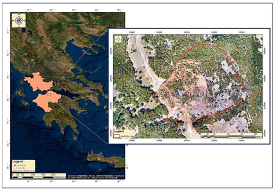
Figure 1.
Location of the study area. The orange color represents the boundaries of the region of Western Greece, while the red dot and the blue rectangular display the location of the city of Patras and the study area, respectively.
A live video footage was captured at the moment of sliding and provides significant details for the landslide evolution. According to this video and along with witnesses from locals, a large volume of loose soil and rock land started moving downslope deforming the northwestern part of the landslide, while a few seconds later, a much larger volume of moving coarse debris modified the southern part of the landslide. These two parts of the landslide present characteristic lithological differentiation: the northwest part includes primarily siliciclastic and/or siliceous lithology, while in the southeast, the prevailing lithology is limestone. However, although the progressive initiation of the phenomenon started from northwest to southeast in different lithology, ultimately, the landslide shows a typical elliptical pattern with an almost identical rupture and landslide zone. The Moira landslide is overall classified as a composite slide.
The general principle for the occurrence of landslides states that they are caused when gravity or other shear forces within a steep slope overpass the shear strength of the formations. In particular, the strength of the Moira landslide material weakened due to rapid snow melting and thus the power that holds the rocks or the soil grains together was reduced, allowing the forces of gravity to move it. After the occurrence of the landslide the main road, which connects the city of Patras with the nearby mountainous settlements was destroyed and covered by the displaced material. The debris material is lying between 685 and 775 m, consisting of reddish loose materials of siliciclastic deposits, compact formations of siliceous rocks, and cobbles to boulders of limestones.
3. Materials and Processing Methodologies
3.1. Materials
Our data set consists of repeated UAV flights and contemporaneous measurements of a GNSS network. The measurements were performed once per month for the time window starting from January 2017 until July 2018. During this specific period, the measurements were dense in time to ensure full monitoring of the landslide’s activity and to mitigate the risk in a possible reactivation. The analysis of the data, collected during these 17 months, revealed that the landslide moves particularly slowly, and therefore we accordingly modified the campaign’s repeatability to three times per year for 2019 and twice per year for 2020. The dates of the repeated UAV and GNSS campaigns are presented in Table 1.

Table 1.
Unmanned aerial vehicles (UAV)-global navigation satellite system (GNSS) campaigns, characteristics of UAV flights, and pixel size of orthophotos and digital surface models (DSMs).
UAV flight campaigns were operated utilizing commercial DJI UAVs (Matrice 600 and Phantom 4). As mentioned in studies [28], using SfM photogrammetry should include diverse specifications about the sensors used (e.g., model, sensor size, image size, sensor shutter type, etc.). Matrice 600 is equipped with a X5 camera which captures images at 16Mp analysis resulting to photos of 4608 × 3456 pixels. Phantom 4 is equipped with a 12.4 MP camera resulting to photos of 4000 × 3000 pixels respectively. Both cameras use electronic shutters. Each flight executed with the same flight grid and the exact same ground control points were used. The corresponding flight characteristics were applied to all acquisitions (Figure 2) (Table 1) at an altitude of 110m above the ground level. Each acquisition of photos took place with a 90% along and 75% across the track overlap of photos. The photogrammetric processing of UAV data was performed into Agisoft PhotoScan software and led to the creation of orthophotos and DSMs with 4 cm spatial resolution. More details on photogrammetric procedure are described in the next section.
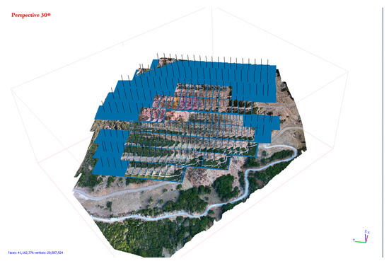
Figure 2.
Flight grid.
In addition, hundreds of static measurements were executed during the repeated GNSS campaigns. The measurements were performed at permanent pillars utilizing a Leica GS08 GNSS Receiver (Figure 3). The pillars are located both inside and outside of the instability zone, in order to ensure a comprehensive monitoring of the activity and the kinematics of the landslide as well as to verify the results of the photogrammetric processing. In that context, 13 permanent pillars were installed at these specific locations, aiming to perform the repeated measurements of a network in exactly the same position (Figure 4). The network included 10 pillars inside and 3 outside the landslide. In more details, the pillars (monuments) of this study were constructed by excavating a hole in loose to rocky soil within or outside the landslide. In the hole, we drove a vertical steel rod. The hole is 15 cm in diameter and 80–100 cm deep depending on the lithology in each position. The steel rod is 1.5 cm thick and 120 cm long with a pointed edge (Figure 3). The rod was driven into the centre of the hole until its top was slightly above the surface, and the edge was driven until refusal wherever possible. Moreover, a 10 cm in diameter PVC tube was placed around the steel rod. The space between tube and soil was filled to the surface with concrete, while the PVC tube was filled with gravel [29]. The GPS antenna mounts on top of the rod directly on the pillar or using a 1 m long extension (Figure 3).
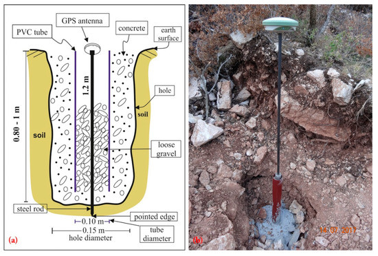
Figure 3.
(a) Sketch showing the different parts of the pillar assembled by the steel rod and a PVC tube. The sketch is not to scale. (b) Photo of a representative pillar (monument) during the July 2017 campaign.
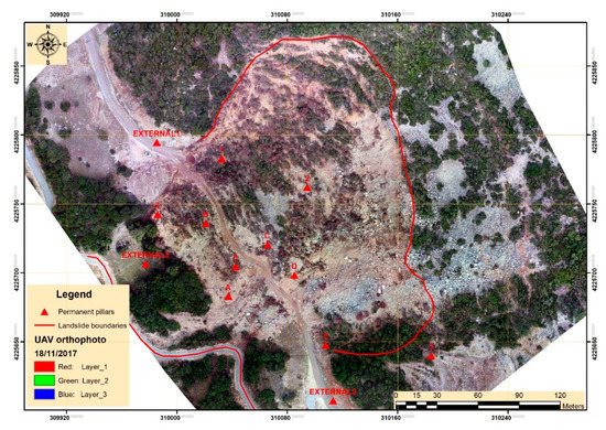
Figure 4.
Locations of the permanent pillars.
3.2. Methods
The framework of the methodology applied in this specific research is as appear in Figure 5. As already mentioned, the objective of this research was the integrated investigation of an active landslide on the base of detail mapping of the landslide and the continuous monitoring for the determination of its activity. Thus, the multidate UAV and GNSS data were processed, and then the results were associated with geological data.
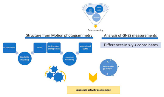
Figure 5.
Flowchart representing the applied methodology.
In detail, UAV data processed according to the structure from motion (SfM) photogrammetric technique. SfM constitutes a low-cost and user-friendly technique which combines photogrammetry and computer vision for 3D reconstruction of an object or a surface model [30,31,32]. The technique is based on similar principles as stereoscopic photogrammetry; however, the geometry of scenes, the orientation, and camera positions are solved simultaneously and automatically, without defining a network of targets with already known 3D positions. Therefore, a series of 2D, overlapping, offset images are utilized along with a highly redundant bundle adjustment, which performs automatic feature matching, in order to create high-resolution 3D structures. In our case, SfM procedure took place in Agisoft PhotoScan software, and high-resolution orthophotos and DSMs covering the study area were generated. The highest-quality option was used for the alignment of the photos. According to the Agisoft manual [33], higher accuracy settings help to calculate more accurately the camera positions but dramatically increase the processing time. High accuracy option means that the software processes the photos at the original size, while the medium, low, and lowest options cause image downscaling by factor of 4, 16, or 64, respectively. By contrast, the highest accuracy setting upscales the image by factor of 4. Since the positions of tie point are chosen on the basis of feature marks detected on the original images, it could be important to upscale the original photo to accurately locate a tie point. Respectively, during the dense point-cloud generation, the ultra-high-quality option leads to processing of original photos, while each lower-quality option implies preliminary image size downscaling by factor of 4 (2 times by each side). As the highest quality options were used in photos alignment, dense point cloud, and mesh generation, we managed to create orthophotos and DSMs with the exact same pixel size. The combination of the 110 m flight altitude above ground level with the 16MP camera of the Matrice produced a 2.8 cm pixel size, while the 12.4 MP camera of Phantom 4 produced a pixel size of 3.8 cm. In order to be able to compare the data from the two different UAVs, we decided to produce orthophotos and DSMs with a pixel (ground sampling distance) of 4 cm (Table 2). Then, these products were further processed by applying different approaches in ESRI ArcGIS environment.
Table 2.
Dates of UAV-GNSS campaigns.
Concerning GNSS data, we established a new low-cost technique network for the estimation of the direction and the rate of movement of the landslide. In particular, the repeated measurements are displayed in a vector format in a three-axis diagram and the vector arrows correspond to the differentiation that occurred in the initial measurement (Figure 6). The plot of the measurements was implemented using MATLAB software. As it can be observed, the measurements at the external pillars (named external 1, external 2, and external 3) have been depicted as points since no movement occurred. In addition, the measurements of pillars called 3, 4, and E display small displacements, while B, C, D, and 5 pillars seem to move more. The larger displacements appeared in the GNSS measurements located at pillars named 1, 2, and A. It is worth mentioning that the direction of movement at pillar A is different from the other pillars. This out of sequence movement is considered as the result of the pillar position. The specific pillar is located lower than the dirt road, and its movement is probably affected by the human activities rather than by the landslide evolution. Materials from the dirt road widening are deposed lower in the slope affecting the pillar A. Moreover, the evolution of the variations in x, y, and z-coordinates of the permanent pillar D during 2017–2020 is given as an example in Figure 7. The x-axis of the diagram represents the multidated GNSS measurements, while the y-axis is occupied by the values of difference in meters.
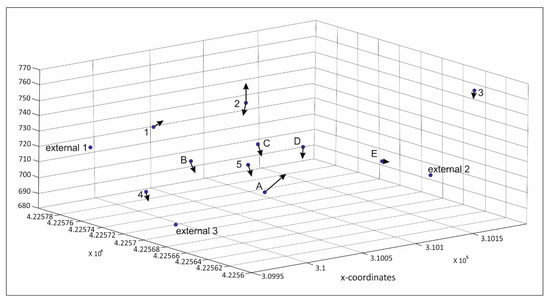
Figure 6.
The results of the repeated GNSS measurements as displayed in a vector format in a three-axis diagram.
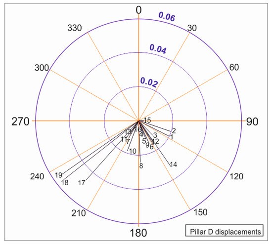
Figure 7.
A polar network presenting the evolution of the displacements of the permanent pillar D during 2017–2020.
4. Results
4.1. Mapping
4.1.1. Orthophotos
Our initial stage of this research is to determine the area affected by the landslide. Thus, a prelandslide orthophoto from the Hellenic Cadastre covering our study area was compared to a postlandslide orthophoto derived from a UAV campaign. In particular, the first UAV flight a few days after the landslide took place on 28 January 2017. The comparison of these two orthophoto maps is used to define the boundary of the landslide which is displayed in red color in Figure 8.
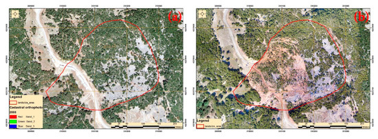
Figure 8.
Landslide area. (a) Orthophoto of Hellenic Cadastre before the landslide. (b) UAV orthophoto after the occurrence of the landslide on January 28, 2017.
It is worthwhile to mention that the procedure of detailed mapping of the landslide’s boundaries as well as any possible change that occurred within the area and potentially affects it, continued throughout the monitoring. Figure 9a presents the landslide area as it emerged from the derived orthophoto. In the next few days, as the road was hidden by the shifted material, a dirt (earth) road was formed through the landslide material in order to connect the city of Patras and the mountainous settlement of Moira (Figure 9b), while a secondary alternative road was constructed along the toe of the landslide (Figure 9c). In addition, a large-scale restoration process was implemented in mid-2018 in the wider area of the road (Figure 9d). This restoration included the widening of the dirt (earth) road.
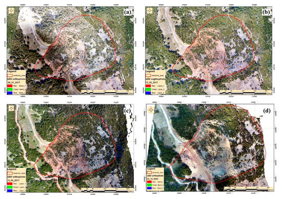
Figure 9.
Continuous mapping of the landslide area. (a) UAV orthophoto on 28 January 2017. (b) UAV orthophoto on 15 February 2017. (c) UAV orthophoto on 13 April 2017. (d) UAV orthophoto on 23 December 2020. Red arrows show the direction of the movement.
Moreover, the extents and volumes of change within the slide have been measured utilizing the cut and fill tool of ArcGIS software. The tool contrasts two surfaces at different time periods, and then it identifies parts where the surface material has been removed or added as well as regions that have not been modified [34]. In detail, we used a prelandslide and a postlandslide orthophoto maps to recognize the surface subsidence and uplift of the landslide (Figure 10). The green color depicts regions of erosion (material removal), while the red corresponds to accumulation of the landslide material. Regions that have not changed are highlighted in grey shade. Then, we calculated the area of each region and the volume of the modified material (Table 3) using the following formula (Equation (1)):
Volume = (area) × (Zbefore − Zafter)
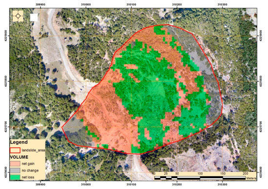
Figure 10.
Map of the landslide showing volume loss (green colored area), volume gain (red colored area), and stable areas (grey color).
Table 3.
Calculation of the area and the volume of the regions, resulted from cut-fill tool.
The results of the Table 3 indicate the balance between erosion (material removal) and accumulation zones in the landslide both in area and volume. This coincidence between volume gain and loss is expected as the Moira landslide toe area ended about 100 m above the Glafkos river and the landslide zone is almost identical with its rupture zone and the in-place deposits. For the use of the terms of landslide and rupture zones, we use the definitions by [35].
4.1.2. Digital Surface Models (DSMs)
Furthermore, we compared two DSMs, one prior to the slide and another one afterwards to determine surface changes. We drew sections throughout the landslide area (Figure 11), and we generated elevation profiles. The blue line depicts the elevation outline prior to the landslide, whilst the red corresponds to the aforementioned outline a few days after the event (Figure 12 and Figure 13). It is obvious that a removal of surface material is detected in the crown area of the landslide, whilst mass was deposed at the toe of surface of rupture of the landslide, corresponding to about 10 m of accumulation of material. Based on this, along with the use of simple mathematical calculations, we estimated that 22.976 m3 of displaced material covered the preexisting road.
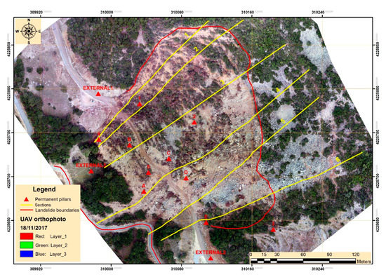
Figure 11.
Distribution of sections within the study area.
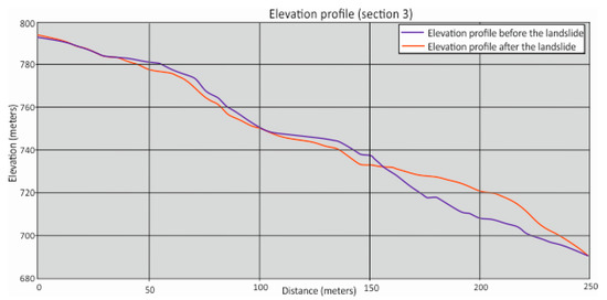
Figure 12.
Elevation profiles of section 3 in Figure 11.
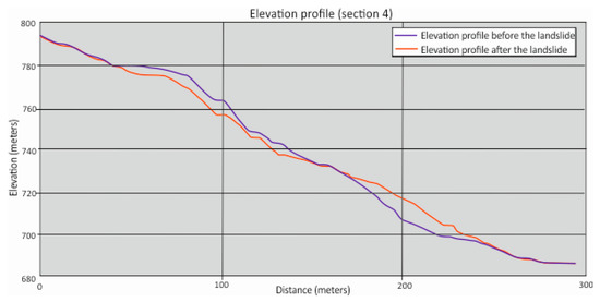
Figure 13.
Elevation profiles of section 4 in Figure 11.
4.2. Monitoring
4.2.1. Orthophotos
Our second concern was the continuous monitoring of the landslide area. The orthophotos resulting from the SfM processing procedure were imported in an ArcGIS environment in order to conduct its area changes. Specifically, the boundaries of the landslide were digitized aiming at the assessment of the change of the landslide over time. Digitization was based on the mapping of the landslide boundaries as well as the subsequent existence of new cracks. Figure 14 displays the evolution of the extent of the landslide from 2017 until 2020. Thus, the blue lines in Figure 14a depict the initial landslide boundaries and the displaced material as well as the boundaries of the earth road, which was constructed a few days after the landslide aiming at restoration of the circulation between Patras and Moira. The orange lines in the Figure 14b annotate the corresponding boundaries and the earth road as mapped on 19 March 2019. Based on the data of the optical imagery and their processing, the areas that display no change over time and areas where the changes are significant, e.g., the subareas A and B, can be observed. In more detail, the in situ observations as well as the analysis of the GNSS data and UAV imageries during these three years revealed that the landslide area is progressively changing at a particularly slow pace. Nevertheless, areas exhibiting change are associated with two distinct mechanisms: landslide remobilized material and translation and break up of blocks and human activity as well. Thus, subarea A was affected by both human activity and remobilized landslide materials (Figure 14c,d). As already mentioned, after the occurrence of the landslide in January 2017, the earth road was opened and restored several times while the potentially unstable landslide material on its border was removed and deposited in new locations. In that context and along with the local topography, the movement of runoff water was facilitated through the formation of temporary surface streams and therefore the landslide material was weathering more easily. On the other hand, the evolution of landslide’s extent in the subarea B is associated with vegetation loss, arising from the creation of new cracks (Figure 14e,f). Thus, the ongoing activity of the landslide is reflected in the presence of dry trees or the deforestation of landslide rupture area.
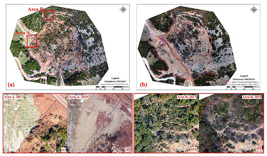
Figure 14.
The evolution of the extent of the landslide between 2017 and 2019. (a) The landslide boundaries in 2017. (b) The landslide boundaries in 2019. (c,d) The evolution of the extent of the landslide between 2017 and 2019 in area A. (e,f) The evolution of the extent of the landslide between 2017 and 2019 in area B.
In addition, the comparison between the different orthophotos took place utilizing the zonal change detection algorithm implemented in ERDAS IMAGINE software. The specific algorithm is able to compute the change between two layers through the application of a pixel-over-pixel comparison. The values range between 0 and 1. The minimum value corresponds to no change, while value 1 corresponds to the maximum change. The greatest differences are imprinted in red shades and are presented in the area of the destroyed asphalt road and the toe of the landslide (Figure 15). Some minor changes are detected close to the crown of the landslide. It is quite characteristic that the new road constructed outside of the landslide zone presents the higher values.
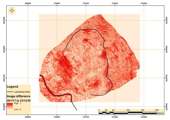
Figure 15.
Difference between the orthophotos of 28 January 2017 and 23 December 2020.
Moreover, the vegetation variations between 2017 and 2020 were digitized in ArcGIS environment and are displayed with orange outline in Figure 16. The digitization was implemented with visual criteria and therefore was focused on areas where extended vegetation variations occurred, since it was easier to recognize them. Areas that lost their vegetation were calculated, corresponding to approximately 2366 m2. The greatest vegetation losses are located in the area near the earth road and southwestward of it.
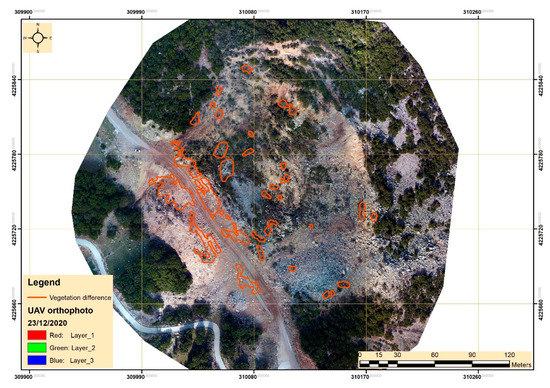
Figure 16.
Digitized vegetation differences between 2017 and 2020.
4.2.2. Digital Surface Models (DSMs)
The derived DSMs were utilized for the detection of surface changes. In more details, elevation profiles were created from the sections which were drawn transversely to the landslide crown (Figure 11). The visualization of all the profiles in a diagram was complex and illegible for the readers; therefore, we present here two representative profiles. In these profiles the dark-green line reciprocates at the elevation outline before, whilst the magenta one represents the same outline on 18 December 2019 (Figure 17 and Figure 18). In terms of comparison, the elevation profiles of 28 January 2017 (dark green) and 18 December 2020 (magenta) exhibited local differences, which were either significant or negligible. The variations in the upper part and main body of the landslide area are related to erosion processes and vegetation changes. Furthermore, the peaks which appeared in the profile of November 2017 and switched to smoother in the corresponding profile of December 2019 are intertwined with the loss of vegetation. It is worth mentioning that the greatest differences are identified again in the wider area of the earth road, where the multidate restoration processes took place. These differences were estimated at about 5 m and are in line with the field observations (Figure 19).
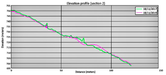
Figure 17.
Elevation profiles of section 2 in Figure 11 on different dates.
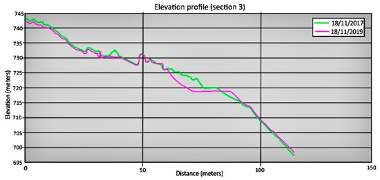
Figure 18.
Elevation profiles of section 3 in Figure 11 on different dates.
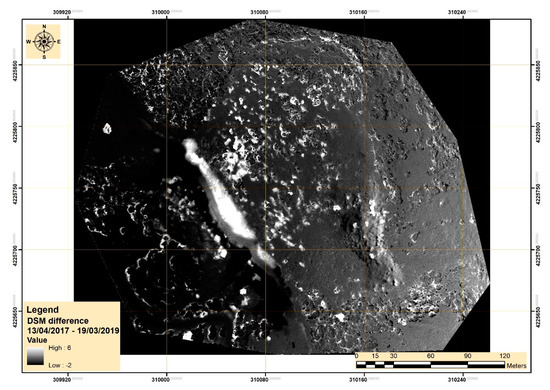
Figure 19.
DSM difference between the DSMs of 13 April 2017 and 19 March 2019.
At the same time the identification of surface changes within the landslide area between 2017 and 2020 was implemented in an ArcGIS environment through the estimation of the slope derived from DSMs. The evolution of the slope angle is depicted in Figure 20. These results attest to slope angle decrease in the first year. On the other hand, slope values increased in 2019, and they remained similar during the 2020. Although the reduction of the inclinations was expected, the inclination increase constitutes an unexpected result. We consider that to be the result of the increasing erosion combined the deforestation. Further, variations near the area of the earth road are related as already mentioned with its opening and multidate restoration.
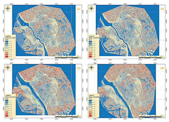
Figure 20.
The evolution of the slope in the study area between 2017 and 2019. (a) The slope of the landslide area in 2017. (b) The slope of the landslide area in 2018. (c) The slope of the landslide area in 2019. (d) The slope of the landslide area in 2020.
Moreover, the UAV point clouds, acquired on 13 April 2017, and 23 December 2020, were imported in Cloud Compare software in order to calculate the distances and therefore surface changes between them. The point clouds were primarily aligned by identifying common points and applying the iterative closest points (ICP) algorithm [36], while the distances were calculated using M3C2 algorithm (Figure 21). The specific algorithm is more suitable for the calculation of distances between two points clouds created by photogrammetric procedure and is more appropriate for areas with complex topography. The calculated distances are ranging from −4 m to 4 m and are in line with the results arising from the other methods.
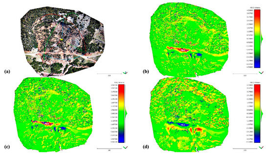
Figure 21.
(a) The point cloud derived from a UAV flight on 13 April 2017. (b) M3C2 distances in x axis calculated between the point cloud of 13 April 2017, and the respective point cloud of 23 December 2020. (c) M3C2 distances in y axis and (d) M3C2 distances in z axis, respectively.
5. Petrographic Analysis
Aiming at understanding the possible role of lithology on the landslide occurrence, we collected a series of samples for petrographic analysis in the laboratory. The sampling strategy was based on the mapping of the landslide showing that the landslide is divided lengthwise into two different lithologies. In the northwest reddish siliceous and siliciclastic rocks are cropped, while in the southeastern part limestones are the predominant lithology. According to the macroscopic description of collected samples from the landslide lithologies, the following materials types have been distinguished: (A) massive pale-yellow or light red limestones (samples LS1 and LS2 respectively) and red crusted laminated limestone (sample LS3). (B) Radiolarites (red colored cherts having conchoidal fracture, samples R1, 2). (C) Loose materials ranging in grain size from fine to coarse (samples LM1, 2) (Table 4). Petrography of the collected rocks was studied on thin sections by a polarizing microscopy. Limestones under polarizing microscope indicated that LS1, 2 samples (Figure 22a,b) were constituted of carbonates (calcite according to X-ray powder diffraction (XRPD) results), with a mainly micritic texture while low amounts of microcrystalline siliceous material as well as veins of sparitic carbonates were also presented. Moreover, secondary minerals such as iron oxides/hydroxides or clays filled pores or microcracks, which was something that was not detected by XRPD analyses. LS3 sample (Figure 22c,d) represented a sparitic limestone with micritic and less siliceous adhesive material and random microveins impregnated with opaque minerals (such as iron oxides/hydroxides). Radiolarites (Figure 23a) were described by a microcrystalline to cryptocrystalline matrix of quartz with characteristic spherical skeletons of radiolarian. Sometimes calcite aggregates or network of carbonates microveins also appeared in the groundmass, assuming the XRPD results (Figure 23b). In addition, secondary clay minerals and opaque ones participated in their bulk compositions reflecting probably weathering phenomena.
Table 4.
Groups of collected rock materials.
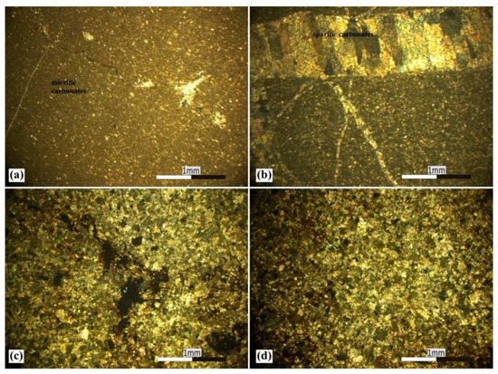
Figure 22.
Representative photomicrographs of limestones. (a): Micritic texture of LS1 sample, in cross polarized light (XPL). Note topically microcracking with black color; (b): Veins with different sizes and orientation filled by sparitic carbonates in a micritic microstructure of LS2 sample (XPL); (c,d): Sparitic to microsparite mainly texture of LS3 sample. Oxides/hydroxides (brown to red colors) impregnated the microstructure, especially along to the microcrackings or pores (black color). Presence in low amounts of siliceous material in micro areas with low birefringence (first order white-grey polarized colors) (XPL).
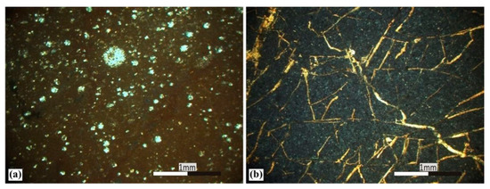
Figure 23.
Representative photomicrographs of radiolarites microstructures. (a): Characteristic spherical skeleton of radiolarian and presence of iron oxides/hydroxides (brown to red colors) in R1 sample (XPL); (b): Network of random microveins filled with carbonates (high birefringence colors) in a siliceous microstructure of R2 sample (XPL).
Mineral compositions of specimens determined by XRPD analyses were presented in Table 5. Prepared random powder samples were slightly pressed into the holders. The scanning area was the 2–70° 2θ, and the step time was 0.015°/0.1 s. The mineral phases were detected by the DIFFRACplus EVA 12® software (Bruker-AXS, Billerica, MA, USA) based on the PDF-2 2006 database. Semiquantitative analyses were done using the abovementioned software and toolbox of peak area calculations. After centrifugation, clay fractions (<2 µm) from selected samples were coated on glass slides and remained in the lab in normal conditions, in order to be observed their behavior after water saturation and drying. Moreover, selected oriented clay fractions specimens were prepared and scanned at 2–30° 2θ, and clay minerals were determined through the XRD patterns (after air-drying at 25 °C and after ethylene glycol treatment and heating at 490 °C for 2 h). Representative qualitative and semiquantitative XRPD analyses results of studied samples are presented in Figure 24a–d and Table 5. The major crystalline detected phase of limestones samples (Figure 24a, Table 5) was calcite (96–99 wt%), as expected, while there were indices of low amounts of quartz (1–4 wt%). Despite the dominant red color of LS2 and LS3 hand samples, the XRPD analyses did not reveal the presence of an iron oxide crystalline phase. This could be explained either by the entrance of iron in the lattice of the detected phases, or to the low amounts of opaque minerals participation (under to the detection limit) or even to their cryptocrystalline/amorphous character. Radiolarite rock samples (R1, 2, Figure 24b, Table 5) were characterized mainly from the expected phase of quartz (87–96 wt%), while significant amounts of calcite participation were detected in R2 sample (11 wt%). Bulk compositions of these materials were completed by low amounts of clay minerals (2 wt%) and oxides (0–2 wt%). In the case of siliciclasatic rocks (Figure 24c, Table 4), the results show that both LM1, 2 assemblages consisted mostly of quartz (86–97 wt%) and less of calcite (0–11 wt%) and clay minerals (3 wt%). XRPD clay fractions analyses of studied materials are presented in Figure 24d. According to those, the clay minerals of smectite and mixed-layer illite/smectite along with illite were consisting of their bulk compositions.
Table 5.
Mineral composition of studied rock materials. Abbreviations: Cc: calcite; Ox: oxides; Qz: quartz; and (-): not detected.
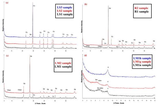
Figure 24.
Representative X-ray powder diffractograms of bulk compositions (a–c) and clay fraction (d) analyses of studied samples. Abbreviations: Cc: calcite; Il: Illite; Sm: smectite, Il/Sm: mixed–layer illite/smectite; Ox: oxides; Qz: quartz; n: air-dried; g: glycolated; and h: heated. Note in Figure 24d of LM1 sample clay fraction analyses, the expected displacement of smectite and illite/smectite peaks, after expanding because ofethylene glycol treatment, as well as the disappearance of smectite and illite/smectite peaks after heating, due to their transformation to illite.
6. Discussion
The provision of knowledge and proper information by researchers or companies regarding landslides is a key issue aiming at mitigating the risk, ensuring human safety and protecting the natural environment and infrastructure. Remote sensing scientists are working towards this direction by developing new, innovative, and promising methodologies. The purpose of this research was the integrated surveying of an active landslide using low-cost and high-repeatability remote sensing data and associating them with GNSS measurements and the petrographic features of the material of the landslide area. The images acquired by commercial UAVs were processed utilizing structure from motion (SfM) algorithm, while the generated high-resolution orthophotos and DSMs were imported in ArcGIS and ERDAS IMAGINE software for further processing. The accuracy of the derived orthophotos and DSMs has already been considered in several studies. These studies examined the accuracy in different scenarios, and it was proven that the products of UAV processing can be used effectively in field research [37,38,39,40].
A continuous detailed mapping of the landslide area was the basis for the monitoring of its evolution throughout these four years. The procedure of mapping included the digitization of the landslide’s boundaries or any other modification progressively occurred within the area in different times. It is worth mentioning, that we calculated the volume change before and after the landslide to have an idea about the amount of the displaced material. In that context, variation in landslide area was detected using DSMs.
The assessment of the activity of the landslide in our study area was implemented by applying different approaches to the orthophotos and DSMs. In that context, a digitization procedure and image difference analysis were applied to the orthophotos, while the creation of elevation profiles and the calculation of the slope were performed on the DSMs. The results demonstrated that the greatest surface changes for the time window starting from 2017 until 2020 are related to three main factors. In particular, erosion processes within the landslide probably related with the differences in lithology, and human activities for the restoration of the road are modifying locally the landslide, while in several places, the vegetation loss appeared to trigger faster erosion and grain coarsening [41]. As already mentioned, GNSS surveys were performed for the validation of the UAV processing results, while a low-cost approach was developed aiming to display the surface movements in vector format in three dimensions. The vector arrows depict the differentiation that occurred in the initial measurement in each GNSS pillar. It is worth mentioning that this early effort worked quite well, and it constitutes a promising approach for tracking the displacements that occur in a landslide. All these results attest to an active landslide, although it is moving particularly slowly. Various researchers [42,43,44,45] extensively analyzed similar natural processes and human activities in landslide areas. Furthermore, there are many studies demonstrating that vegetation can either play a stabilizing role or contribute through its absence to the instability of the area [46,47].
In terms of a more technical perspective for evaluating the applied methodologies, it was observed that the results of UAV data processing are in line with GNSS measurements, which is associated with the high accuracy of the derived orthophotos and DSMs. However, the only limitation on the monitoring procedure was the inability to distinguish the surface changes arising from human activities from those that are related to natural processes. Overall, it is a particularly low-cost approach compared to the traditional geotechnical techniques for landslide monitoring, which require the execution of boreholes and the installation of expensive equipment such as inclinometers. In the proposed methodology, after the initial construction of the pillars the researcher needs a GNSS receiver, a UAV and a high-capacity computer. The total costs for each repeated campaign are limited to the transportation into the field of the personnel and the equipment. The service cost of the equipment (UAV and GNSS receiver) is also negligible.
Regarding the geological structure and the petrographic analysis, the highly deformed limestones and siliciclastic rocks cropping out in the landslide area along with the high amount in participation of low-cohesion loose materials, including smectite and illite/smectite mixed layers, could easily explain the initiation and acceleration of possible new instability phenomena in the future in the Pindos unit [26]. Note that at present it is considered that most of the landslides in Pindos unit are related with the flysch; however, based on the current work it is highlighted for the first time that smectite and illite/smectite mixed layers in the siliciclastic lithologies are probably triggering landslides. The presence of these high-plasticity clay minerals within the siliciclastic rocks under high moisture conditions can be expanded significantly causing landslide occurrence, even if their presence is not in high concentration. Moreover, during period of dry weather smectite type minerals could drastically shrink thus reducing internal friction and cohesion of bulk compositions. Such behaviors were revealed in laboratory, for the representative clay fraction of studied samples, after a cycle of water saturation and consequence drying (Figure 25).

Figure 25.
Demonstration of shrinkage behavior of clay fraction of LM1 sample, (a) after a cycle of water saturation and (b,c) consequence drying at room temperature, due to participation of swelling minerals of smectite and mixed–layer illite/smectite.
The final synthesis of all the results ended up in the identification of different parts within a complex landslide. The northern part of the landslide, which was characterized by higher mobility, landslide material erosion, and deforestation including high-plasticity clay minerals. This is the area where the landslide started and remains the most active part of the landslide through the monitoring period. On the other hand, the southeastern part of the landslide, which covers the wider area of the landslide, is less active and its modification is related with human activity.
7. Conclusions
The current work outlined a low-cost integrated approach for landslide mapping, monitoring and activity determination through the use of data obtained by UAV campaigns and repeated GNSS surveys. The results of GNSS and SfM processing were associated with the petrographic features of the material of the study area. The synthesis of all the applied approaches are concluded in the following remarks:
- Three major lythotypes of limestone and siliciclastic as well as siliceous-rich loose materials were included in the studied landslide.
- The petrographic properties of the siliciclastic rocks appear to play a key role regarding the activity of the landslide, mainly due to the existence of swelling minerals of smectite and mixed-layer illite/smectite. The landslide mass probably moved slipping on one or more saturated clay layers.
- It is a slow landslide which remains active.
- It is affected mainly by natural processed and human activities (road restorations).
- Vegetation loss is related to possible future instability phenomena.
- UAV processing results are in line with the in situ observations and GNSS measurements
- This low-cost methodology of UAV campaigns in combination with GNSS pillars network measurements is considered to be very promising for active landslide monitoring.
- The landslide seems to be stabilized; however we keep on monitoring the area with combined UAV flight campaigns and GNSS measurements.
Future work regarding the low-cost approach for the plotting of the GNSS measurements in three dimensions is needed in order to improve the visualization and to automatize the overall procedure.
Author Contributions
Conceptualization, A.K. and K.N.; methodology, A.K. and K.N.; software, A.K.; validation, A.K., I.K., and K.N.; formal analysis, A.K. and P.L.; investigation, A.K., I.K., K.N., and P.L.; resources, K.N.; data curation, A.K., I.K., K.N., and P.L.; writing—original draft preparation, A.K., I.K., K.N., and P.L.; writing—review and editing, K.N and I.K.; visualization, A.K.; supervision, K.N. and I.K.; project administration, K.N.; funding acquisition, K.N. and A.K. All authors have read and agreed to the published version of the manuscript.
Funding
This research was supported by Grant (80634) from the Research Committee of the University of Patras via “C. Caratheodori” program.
Institutional Review Board Statement
Not applicable.
Informed Consent Statement
Not applicable.
Data Availability Statement
Data available on request due to restrictions. The data presented in this study are available on request from the corresponding author. The data are not publicly available due to public safety reasons.
Acknowledgments
We would like to thank the Research Committee of the University of Patras for funding via “C. Caratheodori” program.
Conflicts of Interest
The authors declare no conflict of interest.
References
- Cruden, D.M.; Varnes, D.J. Chapter 3—Landslide types and processes. In Landslides Investigation and Mitigation; Turner, A.K., Schuster, R.L., Eds.; Special Report 247; Transportation Research Board, US National Research Council: Washington, DC, USA, 1996; pp. 36–75. [Google Scholar]
- Hungr, O.; Leroueil, S.; Picarelli, L. The Varnes classification of landslide types, an update. Landslides 2014, 11, 167–194. [Google Scholar] [CrossRef]
- Niethammer, U.; James, M.; Rothmund, S.; Travelletti, J.; Joswig, M. UAV-based remote sensing of the Super-Sauze landslide: Evaluation and results. Eng. Geol. 2012, 128, 2–11. [Google Scholar] [CrossRef]
- Shi, B.; Liu, C. UAV for landslide mapping and deformation analysis. In Proceedings of the International Conference on Intelligent Earth Observing and Applications, Guilin, China, 9 December 2015; p. 98080P. [Google Scholar]
- Rau, J.Y.; Jhan, J.P.; Lo, C.F.; Lin, Y.S. Landslide mapping using imagery acquired by a fixed-wing UAV. Int. Arch. Photogramm. 2012, XXXVIII-1, 195–200. [Google Scholar] [CrossRef]
- Torrero, L.; Molino, A.; Giordan, D.; Manconi, A.; Allasia, P.; Baldo, M. The Use of Micro-UAV to Monitor Active Landslide Scenarios. In Engineering Geology for Society and Territory; Lollino, G., Manconi, A., Guzzetti, F., Culshaw, M., Bobrowsky, P., Luino, F., Eds.; Springer: Cham, Switzerland, 2015; Volume 5. [Google Scholar]
- Peterman, V. Landslide activity monitoring with the help of unmanned aerial vehicle. Int. Arch. Photogramm. Remote Sens. Spat. Inf. Sci. 2015, XL-1, 215–218. [Google Scholar] [CrossRef]
- Lindner, G.; Schraml, K.; Mansberger, R.; Hübl, J. UAV monitoring and documentation of a large landslide. Appl. Geomat. 2016, 8, 1–11. [Google Scholar] [CrossRef]
- Rossi, G.; Tanteri, L.; Tofani, V.; Vannocci, P.; Moretti, S.; Casagli, N. Multitemporal UAV surveys for landslide mapping and characterization. Landslides 2018, 15, 1045–1052. [Google Scholar] [CrossRef]
- Yaprak, S.; Yildirim, O.; Susam, T.; Inyurt, S.; Oguz, I. The Role of Unmanned Aerial Vehicles (UAVs) in Monitoring Rapidly Occuring Landslides. Nat. Hazards Earth Syst. Sci. Discuss. 2018, 2018, 1–18. [Google Scholar]
- Peppa, M.; Mills, J.; Moore, P.; Miller, P.; Chambers, J. Accuracy assessment of a UAV-based landslide monitoring system. Int. Arch. Photogramm. Remote Sens. Spat. Inf. Sci. 2016, XLI-B5, 895–902. [Google Scholar] [CrossRef]
- Nikolakopoulos, K.G.; Kavoura, K.; Depountis, N.; Argyropoulos, N.; Koukouvelas, I.; Sabatakakis, N. Active landslide monitoring using remote sensing data, GPS measurements and cameras on board UAV. In Proceedings of the Earth Resources and Environmental Remote Sensing/GIS Applications VI, Toulouse, France, 22–24 September 2015; Volume VI, p. 96440E. [Google Scholar]
- Turner, D.; Lucieer, A.; De Jong, S.M. Time Series Analysis of Landslide Dynamics Using an Unmanned Aerial Vehicle (UAV). Remote Sens. 2015, 7, 1736–1757. [Google Scholar] [CrossRef]
- Brook, M.S.; Merkle, J. Monitoring active landslides in the Auckland region utilising UAV/structure-from-motion photogrammetry. Jpn. Geotech. Soc. Spéc. Publ. 2019, 6, 1–6. [Google Scholar] [CrossRef]
- Carey, J.A.; Pinter, N.; Pickering, A.J.; Prentice, C.S.; Delong, S.B. Analysis of Landslide Kinematics Using Multi-temporal Unmanned Aerial Vehicle Imagery, La Honda, California. Environ. Eng. Geosci. 2019, 25, 1–17. [Google Scholar] [CrossRef]
- Eker, R.; Aydın, A.; Hübl, J. Unmanned aerial vehicle (UAV)-based monitoring of a landslide: Gallenzerkogel landslide (Ybbs-Lower Austria) case study. Environ. Monit. Assess. 2018, 190, 28. [Google Scholar] [CrossRef]
- Casagli, N.; Frodella, W.; Morelli, S.; Tofani, V.; Ciampalini, A.; Intrieri, E.; Raspini, F.; Rossi, G.; Tanteri, L.; Lu, P. Spaceborne, UAV and ground-based remote sensing techniques for landslide mapping, monitoring and early warning. Geoenviron. Disasters 2017, 4, 9. [Google Scholar] [CrossRef]
- Cignetti, M.; Godone, D.; Wrzesniak, A.; Giordan, D. Structure from Motion Multisource Application for Landslide Characterization and Monitoring: The Champlas du Col Case Study, Sestriere, North-Western Italy. Sensors 2019, 19, 2364. [Google Scholar] [CrossRef]
- Nikolakopoulos, K.; Kavoura, K.; Depountis, N.; Kyriou, A.; Argyropoulos, N.; Koukouvelas, I.; Sabatakakis, N. Preliminary results from active landslide monitoring using multidisciplinary surveys. Eur. J. Remote Sens. 2017, 50, 280–299. [Google Scholar] [CrossRef]
- Al-Rawabdeh, A.; He, F.; Moussa, A.; El-Sheimy, N.; Habib, A. Using an Unmanned Aerial Vehicle-Based Digital Imaging System to Derive a 3D Point Cloud for Landslide Scarp Recognition. Remote Sens. 2016, 8, 95. [Google Scholar] [CrossRef]
- Al-Rawabdeh, A.; Moussa, A.; Foroutan, M.; El-Sheimy, N.; Habib, A. Time Series UAV Image-Based Point Clouds for Landslide Progression Evaluation Applications. Sensors 2017, 17, 2378. [Google Scholar] [CrossRef] [PubMed]
- Karantanellis, E.; Marinos, V.; Vassilakis, E.; Christaras, B. Object-Based Analysis Using Unmanned Aerial Vehicles (UAVs) for Site-Specific Landslide Assessment. Remote Sens. 2020, 12, 1711. [Google Scholar] [CrossRef]
- Kyriou, A.; Nikolakopoulos, K. Assessing the suitability of Sentinel-1 data for landslide mapping. Eur. J. Remote Sens. 2018, 51, 402–411. [Google Scholar] [CrossRef]
- Hatzfeld, D.; Pedotti, G.; Hatzidimitriou, P.; Makropoulos, K. The strain pattern in the western Hellenic arc deduced from a microearthquake survey. Geophys. J. Int. 1990, 101, 181–202. [Google Scholar] [CrossRef]
- Kokkalas, S.; Xypolias, P.; Koukouvelas, I.; Doutsos, T. Postcollisional Contractional and Extensional Deformation in the Aegean Region; Special Paper. Geological Society of America: Boulder, CO, USA, 2006; Volume 409, pp. 97–123. [Google Scholar]
- Koukis, G.; Sabatakakis, N.; Nikolau, N.; Loupasakis, C. Landslide Hazard Zonation in Greece. Landslides 2005, 4, 291–296. [Google Scholar] [CrossRef]
- Sabatakakis, N.; Koukis, G.; Vassiliades, E.; Lainas, S. Landslide susceptibility zonation in Greece. Nat. Hazards 2012, 65, 523–543. [Google Scholar] [CrossRef]
- James, M.R.; Chandler, J.H.; Eltner, A.; Fraser, C.; Miller, P.E.; Mills, J.P.; Noble, T.; Robson, S.; Lane, S.N. Guidelines on the use of structure-from-motion photogrammetry in geomorphic research. Earth Surf. Process. Landf. 2019, 44, 2081–2084. [Google Scholar] [CrossRef]
- Malet, J.-P.; Ulrich, P.; Déprez, A.; Masson, F.; Lissak, C.; Maquaire, O. Continuous Monitoring and Near-Real Time Processing of GPS Observations for Landslide Analysis: A Methodological Framework. In Landslide Science and Practice; Margottini, C., Canuti, P., Sassa, K., Eds.; Springer: Berlin/Heidelberg, Germany, 2013; Volume 2, pp. 201–209. [Google Scholar]
- Westoby, M.; Brasington, J.; Glasser, N.; Hambrey, M.; Reynolds, J. ‘Structure-from-Motion’ photogrammetry: A low-cost, effective tool for geoscience applications. Geomorphology 2012, 179, 300–314. [Google Scholar] [CrossRef]
- Micheletti, N.; Chandler, J.; Lane, S.N. Chapter 2—Structure from motion (SFM) photogrammetry. In Geomorphological Techniques; Section 2.2; British Society for Geomorphology: London, UK, 2015. [Google Scholar]
- Eltner, A.; Sofia, G. Chapter 1—Structure from motion photogrammetric technique. In Developments in Earth Surface Processes; Tarolli, P., Mudd, S.M., Eds.; Elsevier: Amsterdam, The Netherlands, 2020; Volume 23, pp. 1–24. [Google Scholar]
- Agisoft (User Manual). Available online: https://www.agisoft.com/downloads/user-manuals/ (accessed on 13 February 2021).
- ArcMap (How Cut Fill Works?). Available online: https://desktop.arcgis.com/en/arcmap/10.3/tools/spatial-analyst-toolbox/how-cut-fill-works.htm (accessed on 8 January 2021).
- Domej, G.; Bourdeau, C.; Lenti, L.; Martino, S.; Pluta, K. Shape and Dimension Estimations of Landslide Rupture Zones via Correlations of Characteristic Parameters. Geoscience 2020, 10, 198. [Google Scholar] [CrossRef]
- Chen, Y.; Medioni, G. Object modelling by registration of multiple range images. Image Vis. Comput. 1992, 10, 145–155. [Google Scholar] [CrossRef]
- Gindraux, S.; Boesch, R.; Farinotti, D. Accuracy Assessment of Digital Surface Models from Unmanned Aerial Vehicles’ Imagery on Glaciers. Remote Sens. 2017, 9, 186. [Google Scholar] [CrossRef]
- Mesas-Carrascosa, F.J.; Rumbao, I.C.; Berrocal, J.A.B.; Porras, A.G.-F. Positional Quality Assessment of Orthophotos Obtained from Sensors Onboard Multi-Rotor UAV Platforms. Sensors 2014, 14, 22394–22407. [Google Scholar] [CrossRef]
- Agüera-Vega, F.; Carvajal-Ramírez, F.; Martínez-Carricondo, P. Accuracy of Digital Surface Models and Orthophotos Derived from Unmanned Aerial Vehicle Photogrammetry. J. Surv. Eng. 2017, 143, 04016025. [Google Scholar] [CrossRef]
- Agüera-Vega, F.; Carvajal-Ramírez, F.; Martínez-Carricondo, P. Assessment of photogrammetric mapping accuracy based on variation ground control points number using unmanned aerial vehicle. Meas. J. Int. Meas. Confed. 2017, 98, 221–227. [Google Scholar] [CrossRef]
- Koukouvelas, I.Κ.; Nikolakopoulos, K.G.; Zygouri, V.; Kyriou, A. Post-seismic monitoring of cliff mass wasting using an unmanned aerial vehicle and field data at Egremni, Lefkada Island, Greece. Geomorphology 2020, 367, 107306. [Google Scholar] [CrossRef]
- Alexander, D. On the causes of landslides: Human activities, perception, and natural processes. Environ. Earth Sci. 1992, 20, 165–179. [Google Scholar] [CrossRef]
- Geertsema, M.; Highland, L.; Vaugeouis, L. Environmental Impact of Landslides. In Landslides—Disaster Risk Reduction; Sassa, K., Canuti, P., Eds.; Springer: Berlin/Heidelberg, Germany, 2008; pp. 589–607. [Google Scholar]
- Jaboyedoff, M.; Michoud, C.; Derron, M.; Voumard, J.; Leibundgut, G.; Sudmeier-Rieux, K.; Nadim, F.; Leroi, E. Human-Induced Landslides: Toward the analysis of anthropogenic changes of the slope environment. In Landslides and Engineering Slopes—Experiences, Theory and Practices; Avresa, S., Cascini, L., Picarelli, L., Scavia, C., Eds.; CRC Press: Boca Raton, FL, USA, 2018; pp. 217–232. [Google Scholar]
- Skilodimou, H.D.; Bathrellos, G.D.; Koskeridou, E.; Soukis, K.; Rozos, D. Physical and Anthropogenic Factors Related to Landslide Activity in the Northern Peloponnese, Greece. Land 2018, 7, 85. [Google Scholar] [CrossRef]
- Cui, P.; Lin, Y.-M.; Chen, C. Destruction of vegetation due to geo-hazards and its environmental impacts in the Wenchuan earthquake areas. Ecol. Eng. 2012, 44, 61–69. [Google Scholar] [CrossRef]
- Kim, J.H.; Fourcaud, T.; Jourdan, C.; Maeght, J.-L.; Mao, Z.; Metayer, J.; Meylan, L.; Pierret, A.; Rapidel, B.; Roupsard, O.; et al. Vegetation as a driver of temporal variations in slope stability: The impact of hydrological processes. Geophys. Res. Lett. 2017, 44, 4897–4907. [Google Scholar] [CrossRef]


Publisher’s Note: MDPI stays neutral with regard to jurisdictional claims in published maps and institutional affiliations. |
© 2021 by the authors. Licensee MDPI, Basel, Switzerland. This article is an open access article distributed under the terms and conditions of the Creative Commons Attribution (CC BY) license (http://creativecommons.org/licenses/by/4.0/).