Partial Least Squares Regression of Oil Sands Processing Variables within Discrete Event Simulation Digital Twin

Abstract

Oil remains a major contributor to global primary energy supply and is, thus, fundamental to the continued functioning of modern society and related industries. Conventional oil and gas reserves are finite and are being depleted at a relatively rapid pace. With alternative fuels and technologies still unable to fill the gap, research and development of unconventional petroleum resources have accelerated markedly in the past 20 years. With some of the largest bitumen deposits in the world, Canada has an active oil mining and refining industry. Bitumen deposits, also called oil sands, are formed in complex geological environments and subject to a host of syn- and post-depositional processes. As a result, some ores are heterogeneous, at both individual reservoir and regional scales, which poses significant problems in terms of extractive processing. Moreover, with increased environmental awareness and enhanced governmental regulations and industry best practices, it is critical for oil sands producers to improve process efficiencies across the spectrum. Discrete event simulation (DES) is a computational paradigm to develop dynamic digital twins, including the interactions of critical variables and processes. In the case of mining systems, the digital twin includes aspects of geological uncertainty. The resulting simulations include alternate operational modes that are characterized by separate operational policies and tactics. The current DES framework has been customized to integrate predictive modelling data, generated via partial least squares (PLS) regression, in order to evaluate system-wide response to geological uncertainty. Sample computations that are based on data from Canada’s oil sands are presented, showing the framework to be a powerful tool to assess and attenuate operational risk factors in the extractive processing of bitumen deposits. Specifically, this work addresses blending control strategies prior to bitumen extraction and provides a pathway to incorporate geological variation into decision-making processes throughout the value chain.

1. Introduction

With conventional oil and gas reservoirs being gradually depleted worldwide, activity in the research and exploitation of unconventional resources has grown exponentially over the past two decades. Global estimates of in-place bitumen and heavy oil resources are on the order of 5.9 trillion barrels (938 billion m³), over 80% of which are concentrated in Canada, Venezuela and the United States [1]. Boasting the largest collection of these deposits globally with approximately 1.7 trillion barrels (270 billion m³) of in-place resources [1], Canada is strategically positioned as an important source of unconventional petroleum products. Of this total, roughly 165 billion barrels (26.3 billion m³) are considered technically recoverable and, thus, correspond to Canada’s estimated remaining established reserves [1]. Unlike traditional light oil well drilling, which will decline over time, forecasts show an overall 12% increase in unconventional petroleum production over the next 30 years, with peak rates reached in 2039 [2].

Bitumen and heavy oil reservoirs typically occur in unlithified sand deposits (also called “bituminous”, “tar” or “oil” sands); however, heavy oil is also found within porous siliciclastic and carbonate host-rock successions due to its relative mobility [1]. These reservoirs are generally heterogeneous, containing a variety of different hydrocarbons across the American Petroleum Institute (API) gravity spectrum (from light oil to bitumen). By definition, heavy oil is marginally less dense than water (0.920 g/mL) and corresponds to API gravities in the range of 10–20°; conversely, bitumen and extra-heavy oils are denser than water with API gravities of less than 10° [1,3]. Crude bitumen and heavy oil resources are lacking in terms of lighter distillates, which significantly reduces their market value; consequently, both must undergo upgrading to increase commercial value and marketability. Upgrading to synthetic crude oil products (~20–40° API) involves the addition of hydrogen in order to attain H:C ratios similar to those of conventional crudes, as well as the removal of impurities such as nitrogen, sulphur, oxygen and heavy metals [1].

The current study is concerned with processes specific to the exploitation of oil sand deposits. Typically, economical oil sands contain on the order of 9–13% bitumen (soluble organic matter), 3–7% water and 80–85% mineral solids and insoluble organic matter [3,4]. Generally, 15–30% of the total solids are fines (mainly clays), less than 44 µm in diameter [4]. Most deposits are comprised of unconsolidated sand “bound” by a matrix of bitumen, with or without secondary cements and clays [3]. Despite broad acceptance of the origin and emplacement of bitumen reservoirs, oil sand deposits are subject to substantial levels of geological uncertainty in terms of host formation characteristics, ore composition, grade and overall processability. All of these process variables are strongly influenced by variable and complex host-formation and hydrocarbon depositional histories, in addition to post-depositional alteration processes such as biodegradation and in situ natural water washing [5,6]. Each of these contributing factors can lead to significant variability in ore feed particle size distributions, host-formation mineralogy and hydrocarbon chemistry and quality, all of which have direct impacts on downstream processing.

As with many types of mining projects, there are a variety of processes along the oil sands value chain; each of these streams may serve a particular function, but also require coordination of inputs and outputs with both up- and down-stream processes. This coordination can be difficult to maintain at times, even for systems that receive relatively stable ore feeds, but is exponentially problematic for projects dealing with heterogeneous ores. For example, blending strategies are common in mining for grade control or to minimize undesirable impurities in ore feeds; however, oil sand operations must also consider factors such as grain size distribution and mineral chemistry in order to regulate the transfer of intermediate products (e.g., slurries or froths) within hydrotransport pipelines. Furthermore, some complex ores may require additional treatment prior to, or between, conventional processing methods. For instance, heavy gas oil phases partitioned by distillation during upgrading are fed to fluid cokers and hydrocrackers to increase H:C ratios and break down long-chain molecules [7]. Similarly, problematic high chloride oil sands, often with elevated clay contents, could require ancillary control strategies (e.g., water content reduction, additives/inhibitors and blending) to reduce corrosive effects or blockages (i.e., ammonium chloride) related to hydrolysis reactions in downstream processes [8,9,10,11].

Improper process control strategies that do not suitably incorporate the geometallurgical profile of source ore feeds can result in major bottlenecks in mining and processing operations, ultimately leading to increased operating costs, decreased efficiencies and, even, potentially important reductions in project life. Several authors have emphasized the importance of establishing alternate modes of operation for mineral processing facilities [12,13]. Alternate modes are designed using mass balance and mathematical programming, and the operational decision to switch between modes is triggered by changing conditions or as critical thresholds are crossed [12,13]. The approach is particularly effective for complex mining systems dealing with heterogeneous ore feed and process variables, as demonstrated by recent studies [14,15,16,17]. Continuous online material and system process monitoring notwithstanding, a natural and powerful extension is to couple the development of operational modes with robust predictive models that benefit from earlier systematic sampling protocols. This type of integrated approach can lead to improved planning and fine-tuning earlier in the value chain, rather than being forced to make continual reactive adjustments based on process outputs (e.g., bitumen recoveries).

Given the high degree of variability inherent to oil sands mining and processing operations, it is evident that appropriate quantitative frameworks are needed in order to monitor system performance and response under changing conditions. One such computational intelligence tool is the digital twin, which is an integrated multidisciplinary probabilistic simulation of a system that uses the best available data models, updates and history to mimic the operational life of the corresponding physical system [18,19]. The development of digital twins using discrete event simulation (DES) is an effective approach because it allows for the simulation of interactions between critical parameters and processes with respect to random natural variations, e.g., geological uncertainty. Furthermore, DES models can also optimize trade-offs between available operational policies, as well as the limits that dictate the timing of their execution [15,16,17]. By simulating extended operating periods, potential deficiencies or bottlenecks in the coordination of system processes can be identified; strategic decisions can then be made to adjust operational policies, accordingly, thereby pre-emptively assessing and managing risk factors. The drive to improve overall system efficiencies is further amplified by increasingly stringent environmental regulations, industry best practices and pressure from community stakeholders.

This work introduces an extended framework capable of integrating predictive modelling using partial least squares (PLS) regression incorporated within a digital twin, for the evaluation of system response to geological uncertainty. A case study using data derived from Canada’s oil sands is presented for a conceptual surface mining operation to assess the effect of implementing potential new ore blending schemes. The initial dataset was kindly acquired through partnerships with the National Research Council Canada (Ottawa, ON, Canada) and Syncrude Canada Ltd. (Research and Development–Edmonton, AB, Canada).

2. Background

2.1. Oil Sands Geology and Petrochemical Processing

Canada’s vast oil sand resources are located almost exclusively in northeastern Alberta, within three core areas, namely the Peace River, Athabasca and Cold Lake deposit regions (Figure 1) [7,20]. Collectively, these accumulations span an area of approximately 142,000 km² [7,21], the largest of which is the Athabasca region, containing ~75% of the provincial reserves [20,22].

Generally, the Alberta oil sands have a thin overburden, and the deposits are concentrated within the early Cretaceous McMurray Formation (Mannville Group), which has variable thickness related to an original depositional surface defined by karstic features in underlying Devonian carbonates [3,4]. The present-day low API oils are the result of degraded Exshaw Shale sourced hydrocarbons [3,23,24]. Ores hosted within the McMurray Formation are subject to heterogeneities and related geological uncertainty, at both regional and individual reservoir scales. Key factors that affect the distribution and chemistry of bitumen include physical reservoir characteristics, mineralogy and mineral chemistry and fluid distribution and chemistry; these attributes are the result of dynamic host-formation and hydrocarbon depositional histories, as well as complex post-depositional alteration processes [6]. For example, though the predominant host successions are thought to have been deposited in estuarine settings, reservoirs have also been identified in fluvial and shallow marine settings, each with differing host porosities and permeabilities, mineral compositions, grain size distributions and related bitumen qualities [3,6,25,26]. Moreover, even broadly mappable geologic sequences (e.g., estuarine settings of the Middle McMurray Formation) may actually consist of multiple events overlapping in space and time, with each contributing several hierarchical heterogeneities [6,27]. Microbial degradation has been strongly linked to the quality of petroleum, having destroyed important proportions of originally emplaced conventional oil through the removal of lighter distillates [4,6]. In situ water washing, which removes the more water-soluble distillates through contact with formation waters, is considered the second most important post-depositional alteration process that affects the geochemistry, quality and bulk physical characteristics of petroleum accumulations [1,5].

Open-pit mining has traditionally been the dominant method implemented in the Alberta Oil Sands Region (AOSR), but in situ production first surpassed surface mining in 2012 and continued this trend into 2013 [1,28]. For aging open-pit mines to remain competitive with the newer in situ operations, they must be ready to implement changes to their process and, thus, adapt to their forecasted feeds. In oil sands surface mining, overburden is stripped, and conventional truck-and-shovel methods are used to excavate the ore, followed by a series of treatments to liberate the bitumen from the mineral grains for subsequent recovery and cleaning. First, the ore is crushed and mixed with water and additives to create a slurry, which is then pumped to the extraction facilities via hydrotransport pipelines [7,20]. Upon exit, the slurry is subject to water addition and gravity-settling separation processes, which produces a bitumen froth, a middlings stream and a first round of tailings. The aerated bitumen froth (comprising ~60% bitumen, 30% water and 10% fine solid particles) rises to the top of the separation vessel, meanwhile flotation cells are used to recover bitumen from the middlings [7]. The separated froth is deaerated and then sent to the froth treatment plant, where the addition of a light hydrocarbon solvent helps reduce the viscosity of the bitumen; this allows for more effective separation of any remaining impurities by centrifugation and inclined plate (gravity) settlers. The final product of this froth treatment process is called diluted bitumen (also referred to as “dilbit”) and is accompanied by another tailings stream.

Depending on the choice of hydrocarbon solvent, the generated dilbit can require further upgrading (typical for naphthenic treatment) or head straight to the refinery market (possible with paraffinic treatment); in either case, the diluent is removed prior to further processing. Lighter hydrocarbon solvents yield cleaner dilbit products by reducing the viscosity of the emulsion, which allows for gravity-based removal of water and solids. Paraffinic solvents promote asphaltene (impurity) precipitation, whereas naphtha cannot do this at practical dilution rates. Upgrading converts viscous, hydrogen-deficient hydrocarbon with elevated impurity levels into high-quality synthetic crude oil products with density and viscosity attributes similar to those of conventional light sweet crude oil [7]. The process first splits the bitumen into hydrocarbon streams (i.e., light and heavy gas oil) in a vacuum distillation unit. The lighter distillates (“tops”) are fed into hydrotreaters for stabilization and impurity removal (e.g., sulphur), meanwhile the heavier phases (“bottoms”) are sent to fluid cokers (thermal conversion units) to remove carbon and to hydrocrackers where hydrogen is added and long-chain molecules are broken down [7].

2.2. Multivariate Statistics and Partial Least Squares (PLS) Regression

Multivariate statistics is a branch of statistics dealing with methods that examine the simultaneous effect of multiple variables [29]. Multivariate techniques extend the approach of univariate and bivariate investigations to include the analysis of covariances (or correlations) that reflect the extent of relationships between three or more variables, as well as similarities indicated by relative distances in $n$-dimensional space [29]. This area of research has expanded greatly over the past few decades due to significant technological advances in computing power and data frameworks.

Partial least squares (PLS) regression is a multivariate statistical method that combines and generalizes features from principal component analysis and multiple linear regression, with the objective of predicting a set of dependent variables from a potentially large set of independent variables [30,31]. The technique was pioneered in the 1960s by Herman Wold for use in the social sciences but has since gained traction in a variety of fields, including chemometrics, sensory evaluation and neuroimaging [30,31,32,33]. It is also becoming popular in the biological and environmental sciences with applications in soil and microbial ecology [34,35], biodiversity [36,37], paleo-climatological reconstruction [38] and ecotoxicology [39,40]. More recent studies in the geological disciplines have identified the use of near-infrared (NIR) or short-wave infrared (SWIR) reflectance measurements to build predictive models of metal concentrations in soils [41,42].

The main underlying computation for PLS is the singular value decomposition (SVD) of a matrix, which gives the best reconstruction (in a least squares sense) of the original data matrix by a matrix of lower rank (dimension reduction), while limiting the loss of significance [43]. The SVD is closely related to the well-known eigen-decomposition for non-symmetric matrices [44]. As a matter of notation, matrices are denoted by upper case bold letters, column vectors by lower case bold letters, and the superscript “$T$” is used to indicate transposition of either. Formally, the SVD of a given matrix, $R$, decomposes it into three matrices, comprising the left singular vectors, the singular values and the right singular vectors, as follows:

$$R=U\Delta V^T={\displaystyle \sum }_l^L{u}_l{\mathsf{\delta }}_l{v}_l^T$$

(1)

where $R$ is the $J\times K$ correlation matrix, derived from the cross-product of the two original data tables (transpose $m\times n$ matrix of the independent variables, $X^T$, and $n\times p$ matrix of the dependent variables, $Y$), as:

$${\displaystyle \sum }_{k=1}^n{x}_{ik}^T{y}_{kj}$$

(2)

$U$ is the $J\times L$ matrix of the left singular vectors ($L$ corresponds to the rank of $R$), $\Delta$ is the $L\times L$ diagonal matrix of the singular values, $V$ is the $K\times L$ matrix of the right singular vectors, and $u_l$, ${\mathsf{\delta }}_l$ and $v_l^T$ are the $l$th left singular vector, singular value and right singular vector, respectively [43]. The non-negative singular values are sorted in decreasing order and represent the maximum covariance between each respective set of left and right singular vectors [45]. Note that both original sets of data are typically made comparable through statistical preprocessing (i.e., mean centering and rescaling each variable).

It is useful to explain the SVD from a geometric perspective as a series of orthogonal axis rotations and scaling of unit matrices about the origin. As shown in the simplified interpretation for a $2\times 2$ matrix (Figure 2; after [46,47]), the SVD can be summarized as a linear transformation composed of three fundamental actions. These actions include: (1) rotation of the right singular vectors $\left\{v_1, v_2\right\}$ of matrix $V^T$ within the original unit sphere; (2) scaling by the singular values $\left\{{\mathsf{\delta }}_1, {\mathsf{\delta }}_2\right\}$ of matrix $\Delta$, which correspond to the length of the principal semiaxes of the new hyperellipse; (3) rotation of the left singular vectors $\left\{u_1, u_2\right\}$ of matrix $U$, oriented along the same principal semiaxes [47,48].

The functional basis of PLS is to relate the information in two data tables that gather measurements on the same set of observations (i.e., samples). The method works by deriving linear combinations of the original variables through the SVD of a correlation matrix, such that covariance is maximized between each pair of the defining latent vectors (implied orthogonality) [43]. These combined variables are also referred to as latent variables, dimensions or components. In PLS regression, the SVD simultaneously decomposes matrices $X$ and $Y$ (by virtue of the correlation matrix $R$) and iteratively computes sets of orthogonal latent variables and the corresponding regression weights [43].

Generally, this entire process is first carried out on subsets of training and validation data (i.e., measured values exist for both independent and dependent variables) to build and evaluate a regression model. The selection of training and validation splits is dependent on a number of factors, including sample population size, the nature and variability of the data and the scope of the prediction problem. Sample splits should generally be selected at random but can also be stratified when there are constraints imposed by different sample types (e.g., rock type); 80–20 training–validation splits are common in practice. Other techniques, such as $k$-fold cross-validation, are also widely popular to further minimize bias; one of these approaches is further detailed in Section 3.2.1. The final regression coefficients are then subsequently applied to a test dataset (i.e., for which data are only available for the independent variables) in order to predict the entire set of dependent variables.

By contrast with standard techniques, PLS regression can be used to predict a whole table of data and can also handle multicollinearity, thereby eliminating the necessity to remove certain predictor variables, which may not be linearly independent and would normally cause overfitting [43]. This is particularly important in the context of mining systems wherein a significant proportion of the data variables used for ore characterization (e.g., geological, geochemical and mineralogical) are intimately linked. For example, ~50% of the variables in the present study are strongly correlated (correlation coefficients > 0.75) with one or more other variables (Appendix A). This multicollinearity among independent variables renders the classic multiple linear regression (MLR) method inappropriate for predictive modelling in most cases due to difficulties in distinguishing the effects of individual variables [49]. This can lead to the inflation of standard errors, which may cause incorrect variable significance classifications and/or numerical instabilities related to the inversion of the covariance matrix ($X^{T}X$) in the calculation of regression coefficients ($B={(X^{T}X)}^{-1}{X}^{T}Y$) [49]. In PLS regression, the multicollinearity problem is bypassed by projecting the original variables to latent structures (linear combinations) and forcing orthogonality between the new variables ($t$ and $u$). The different approaches of MLR and PLS are conceptualized in Figure 3. These attributes make PLS regression a powerful and highly adaptable tool because unlike other methods, it can be used on large datasets with an abundance of variables.

To the best of the authors’ knowledge, there has been very little work done using PLS regression in the areas of mining and system dynamics research to date. The most relatable study successfully developed a predictive model for the amount of kaolinite (clay mineral) in a deposit by linking earlier collected NIR spectroscopic data to confirmatory geochemical data [51]. The current work aims to extend this approach of adapting modern statistical methods for decision-making processes by integrating a predictive PLS model into a digital twin to evaluate operational risks within mining system processes. The digital twin is constructed within a discrete event simulation (DES) framework.

2.3. Digital Twins and Discrete Event Simulations

Digital twins are a form of computational intelligence tool that describe and simulate the comprehensive physical and functional aspects of integrated processes or systems and utilize the most advanced and updated information models available to quantify causal relationships between key variables and parameters [18,19]. Digital twin development using DES is particularly useful in the design and testing of alternative operational policies and associated trade-offs and can be applied to any or all lifecycle phases of an engineering project.

DES frameworks are valuable tools to expedite and support decision making within industrial systems. The key difference between mining and other industrial systems is the notion of geological uncertainty, i.e., the natural variability associated with orebodies and host geological environments. Because DES has the flexibility to incorporate random distributions, i.e., it is a form of Monte Carlo simulation [52], it can be used to evaluate the potential effects of geological uncertainty on mining system dynamics.

Paramount to the development of suitable digital twins is the establishment of alternate modes of operation that can be engaged under changing conditions or as critical thresholds are breeched [12,13]. Geometallurgical units are then defined based on the expected behaviour of classified mining blocks under each of the available modes [12,53,54]. Key performance indicators (KPIs) can also be tracked to observe system response to unexpected trends in ore feed attributes; trade-offs are optimized by adjusting available operational policies and the thresholds that control their timing [15,16,55].

Computer-based DES is a useful risk assessment tool, as it can simulate extended periods of operation to identify potential bottlenecks or other deficiencies; these risk factors can then be mitigated through implementation of operational buffers, such as stockpiling or ore blending strategies. To further support decision making (e.g., installation of new equipment), sets of validation or testing data can also be simulated in order to generate confidence intervals.

In the mining industry, DES frameworks have generally been limited to equipment selection [56], material management [57] and general transportation practices [58]. Applications related to availability and reliability data of mining equipment [59], underground mine refuge station location planning [60] and continuous mine system simulation for short-term planning and decision control [61] have also been explored to a lesser extent.

Recent mine-to-mill modeling studies include quantification of the effects of ore type spectral imaging [62] and evaluation of coupling solar radiation energy with a semi-autogenous grinding (SAG) mill [63]. As previously mentioned, some authors have developed alternate modes of operation for mineral processing via mass balance and mathematical programming [13]. Recent studies have applied this technique to mining contexts using discrete event simulation (DES), including concentrator and smelter dynamics [14,15,55], heap leach processes [16] and tailings retreatment applications [17].

There is a striking similarity between a two-mode mining system model and the RQ problem from inventory theory [15,64]. When inventory levels fall below a given “re-order point”, R (i.e., critical ore level), a replenishment order of quantity, Q, is made prior to stockout. In mining systems, the critical ore level is directly proportional to the expected rate of ore consumption and the lead time required to replenish the stockpile to sufficient levels. However, this relationship does not account for potential natural variation (i.e., geological uncertainty), which could result in either surpluses or shortfalls, the latter of which is a risk for stockout (see Wilson et al., 2021 [17] for examples). This operational risk can be mitigated by raising the critical ore and/or total stockpile target levels, at the expense of higher operating (handling) and capital (equipment/storage) costs. Thus, the two-mode model is important to both risk management and multiobjective optimization (e.g., balancing throughput vs. stockpile management).

This type of framework can be formulated using commercial DES software to simulate extended operating periods and assess the system-wide response to varied stockpile management strategies. Mode A typically represents a consumption phase, whereas Mode B constitutes a phase of replenishment. While the consumption mode is generally more productive, it is not sustainable to activate indefinitely without an alternate mode of replenishment due to stockout risk [15]. The timing for switching between modes is governed by operational policy, which defines threshold crossing events (i.e., critical ore level).

When the critical ore level is raised to act as an operational buffer, this threshold no longer represents a true minimum, as the ore stock may continue to be consumed until the next replenishment mode [15]. This can result in stockout if ore levels are insufficient to last until the next planned shutdown and highlights the importance of building recourse actions into the model. The current framework incorporates blending practices as a control measure in response to geological uncertainty; ore types are blended and processed according to different set proportions (dictated by operational policy) designed to maintain consistent ore feed. In the event of stockout of one of the ore types, contingency modes are enacted until the next planned shutdown and subsequent replenishment phase (depending on mined ore supply).

The current study is an adaptation of recent DES modelling work by Navarra et al. [15,55] and Wilson et al. [17], which focused on the implementation of alternate modes of operation to balance plant ore feed types with respect to system-wide dynamics. By integrating predictive PLS regression modelling into a DES framework, this work demonstrates the potential benefits of using ore characterization data collected at an early stage to evaluate the future performance of system processes under geological uncertainty.

3. Incorporation of Quantitative Methods into Discrete Event Simulation

3.1. Case Study: Predictive and System Process Modelling of Canada’s Oil Sands

An initial dataset derived from Canada’s oil sands was acquired through partnerships with the National Research Council Canada (NRC) and Syncrude Canada Ltd. retrieved from the NRC Office of Energy and Research and Development (OERD) database. The set contains elemental, mineralogical and ore compositional data for a total of 60 samples collected from multiple sources in the AOSR. Of the total number of samples, 40 were sourced from various locations at the Syncrude operations, and permission has been graciously granted to include these in the present conceptual study. The remaining 20 samples come from a number of miscellaneous sources as part of smaller studies and are already available to the public domain.

Ore compositions (i.e., bitumen, water and solids contents) were analyzed by the standard Soxhlet-Dean and Stark method [65]. Separately, splits from the original sample material were prepared for subsequent analytical determinations using a micronizing procedure recently developed at NRC. In this method, ore samples are first homogenized with a spatula at room temperature; isopropanol (4 mL) and toluene (6 mL) are then added to an aliquot (~2–3 g) and micronized with agate beads in a McCrone micronizing mill. The contents are strained into a weighed petri dish (any remainder is carefully rinsed with isopropanol and toluene) and allowed to dry for 24 h in a fume hood prior to weighing. Lastly, the dried mixture is scraped and transferred for further homogenization using a mortar and pestle. Elemental compositions were determined by wavelength dispersive X-ray fluorescence (WD-XRF) using a fusion-based procedure [66] and CHNS measurements by combustion technique using an automatic elemental analyzer (Elementar Vario EL Cube) for carbon and sulphur. Mineral phase ratios were acquired by X-ray diffraction (XRD) with Rietveld refinement carried out on random orientation powder mounts. The mounts were prepared using a zero-background specimen holder (Si crystal, P-type, B-doped) with a cavity diameter of 20 mm and thickness of 0.2 mm; a glass slide was used to remove excess powder and create a flat surface. Final mineralogical compositions were based on the combined XRF, CHNS and XRD results and determined using the NRC-developed quantitative phase analysis (QPA) methodology parameterized with singular value decomposition (SVD), collectively termed SVD-QPA [67].

Basic descriptive statistics were computed to summarize the original raw dataset (

Table 1. Summary of descriptive statistics for mineral phases analyzed by X-ray diffraction (XRD) in 60 samples.

	Mineral Phase Concentrations (wt.%)
Mineral	Max	Min *	Median	Mean	Standard Deviation	Variance
Quartz + silica	87.94	33.30	77.43	74.96	11.22	125.82
Illite	25.63	0.01	5.31	5.89	5.20	27.06
Kaolinite	24.09	−1.49	2.18	3.90	5.15	26.48
Chlorite	1.42	−1.09	0.01	0.10	0.37	0.14
Calcite	3.15	−1.06	0.01	0.09	0.50	0.25
Dolomite	8.21	−0.03	0.12	0.83	1.69	2.85
Ankerite	0.98	−0.03	0.01	0.05	0.16	0.03
Siderite	5.09	0.00	0.61	1.04	1.15	1.33
Pyrite	1.05	−0.05	0.04	0.16	0.23	0.05
Zircon	0.44	0.00	0.06	0.09	0.08	0.01
Rutile	0.62	0.03	0.13	0.15	0.09	0.01
Anatase	1.13	0.00	0.11	0.26	0.29	0.09
Ilmenite	0.05	0.00	0.01	0.02	0.01	0.00
Lepidolite	0.05	0.00	0.01	0.02	0.01	0.00
Gypsum	0.29	−0.85	0.01	0.01	0.13	0.02
Bassanite	0.30	−0.90	0.01	0.01	0.14	0.02
Anorthite	3.65	−7.14	0.12	0.22	1.22	1.49
K-feldspar	4.16	−0.35	1.06	1.19	0.86	0.74
Albite	11.38	0.00	0.34	0.96	1.75	3.08
Iron oxide + hydroxide	5.25	−1.75	0.10	0.19	1.07	1.15
Apatite	0.49	0.00	0.05	0.10	0.09	0.01
Cristobalite	0.10	0.00	0.01	0.01	0.02	0.00
Organic carbon	13.15	0.58	8.24	7.63	3.18	10.09
Organic sulphur	1.03	−0.17	0.39	0.38	0.27	0.07

* Negative values are related to the SVD-QPA methodology used for mineralogical composition reconstruction based on combined experimental results from elemental concentrations by XRF (Si, Al, K, Mg, Fe, Ti, Zr, Mg, Ca and P), carbon and sulphur contents and mineral ratios determined by Rietveld analysis of XRD powder patterns [67]. The vast majority of these are well within tolerance; the anomalous value noted for anorthite (minimum of $-7.14$) can be linked to a specific sample likely containing Ca-bearing smectite, which was not one of the defined phases in the QPA due to low overall Ca phases in the analyzed sample population.

and

Table 2. Summary of descriptive statistics for elemental and ore compositions analyzed by X-ray fluorescence (XRF) and Soxhlet-Dean and Stark extraction (respectively) in 60 samples.

	Elemental Compositions (wt.%)
Element	Max	Min	Median	Mean	Standard Deviation	Variance
Na	1.00	0.00	0.03	0.08	0.15	0.02
K	2.00	0.09	0.55	0.64	0.43	0.18
Si	42.01	26.75	38.42	37.98	2.77	7.69
Al	9.09	0.00	1.56	2.22	2.09	4.36
Fe	3.21	0.00	0.54	0.72	0.66	0.44
Mg	1.09	0.00	0.05	0.12	0.22	0.05
Ca	3.49	0.03	0.16	0.30	0.56	0.31
Ti	0.72	0.02	0.20	0.25	0.17	0.03
Zr	0.22	0.00	0.03	0.04	0.04	0.00
P	0.09	0.00	0.01	0.02	0.02	0.00
C	13.29	1.08	8.38	7.86	3.05	9.32
S	1.31	0.05	0.47	0.47	0.28	0.08
	Ore Compositions (wt.%)
Phase	Max	Min	Median	Mean	Standard Deviation	Variance
Bitumen	16.28	0.00	9.53	9.16	4.48	20.04
Water	19.57	0.41	5.63	6.65	4.37	19.06
Solids	91.25	76.79	83.97	84.42	2.86	8.16
Fines	99.46	1.36	24.80	34.22	27.01	729.80

), which consists of data for 12 elements, 24 mineral phases and compounds and 4 oil sand constituents (bitumen, water, solids and proportion of fines).

The data are highly heterogeneous and reflect ores likely hosted by formations spanning mainly estuarine and shallow marine settings, with a small number possibly from fluvial settings. Because information on sample provenance was fairly limited, assumptions had to be made in order to classify sample points for the sake of this conceptual study. This actually works out reasonably well, as it highlights the importance of systematic data collection and demonstrates the powerful information that can be gained by integrating properly developed geometallurgical profiles into advanced quantitative frameworks and digital twins.

In positing the depositional settings from which the majority of the oil sand samples came, the data were sorted based on total clay contents (illite–kaolinite–chlorite) and a cut-off level of 6 wt.% was applied; samples with less than this limit were classified as (fluvio-)estuarine and those with greater as marine. A broad inverse relationship is also evident in the data between total clay and bitumen contents, consistent with previous studies. Given that bitumen contents are generally higher in ores from fluvial and estuarine settings than those from marine settings [7], this relationship could serve as a useful check of the viability of assumed provenances. Bitumen contents in the classified (fluvio-)estuarine samples average 11.74 wt.% (standard deviation of 2.81 wt.%), which coincides with the stated range of ~9–13% for economic ores [3,4]. The average bitumen content for marine samples is 6.52 wt.% (standard deviation of 4.52 wt.%), consistent with borderline uneconomical ores [7,68]. Overall, the assumed depositional types appear fairly reasonable compared to natural deposit settings and related variations.

The dataset was also expanded to include postulated bitumen recovery data that were mostly unavailable. To this end, batch extraction unit (BEU) test data for 5 estuarine and 5 marine ore samples from previous work [69,70] were used to calculate appropriate bitumen recovery distributions for each depositional type. By applying these respective sample population means and standard deviations to a random number generator, reasonable spreads of recovery data were inferred for each sample type. This was deemed necessary in order to classify ore types based on both depositional setting (clay content) and generally related ore processability, for subsequent predictive and system process modelling (Section 3.2.1 and Section 3.2.2, respectively). It is notable that the effect of fines on bitumen recovery can vary considerably depending on the type of fines and water chemistry [7]; studies have shown a depressive effect in the presence of degraded illite or smectitic clays [71], as well as ultrathin illite [69] and interstratification [72].

For the purposes of this study, all samples are being treated as though they were sourced from a single mining project, with each of 20 mining parcels (i.e., blocks) corresponding to a minimum of 3 oil sands samples. The initial concept is to develop effective predictive models using PLS regression such that bitumen recoveries could be estimated with confidence earlier in the value chain. Subsequent incorporation of these predicted data into DES frameworks would then expedite the evaluation of system response to geological uncertainty caused by heterogeneities in source ore feeds.

To demonstrate the overall concept, the classified ore types are blended according to two different schemes established through mass balancing and mathematical programming. Each of these schemes corresponds to a separate operational mode, whereby the primary blend is considered the productive phase, and the secondary blend is considered a replenishment phase. The mining parcel data, classified into proportions of each ore type, are then incorporated into a DES framework to simulate system response to ore feed availability for a designated tonnage of oil sands to be processed; bottlenecks or stockout risk for either ore type can be identified and adjustments made to the potential modes of operation (Figure 4).

Notably, since fines content is generally linked to geological setting and processability, a classification scheme based on depositional setting (and predicted recovery) actually runs in parallel to a process recently developed by Syncrude for the control of solids distribution in a bitumen froth [73]. Under this patented methodology, coarse oil sands (which normally produce high bitumen recoveries) are blended with high-fines material prior to extraction in order to improve the efficiency of pipeline transport from remote extraction sites to the froth treatment plant (Figure 5) [73]. As a result, the current framework could help quantify the effects of different ore blending strategies on downstream system processes and better guide the implementation of alternate operational modes.

This type of integrated quantitative framework allows for well-planned adjustments to process control strategies (e.g., ore blending), thereby streamlining risk-based decision making, increasing efficiencies and, likely, extending operational life through improved mine planning. The approach requires extensive sampling coupled with detailed analytical work initially, particularly in newly discovered or poorly characterized resource areas. With a sufficiently large population of sample points, robust predictive models can then be developed and implemented with confidence; at this stage, the expensive and time-consuming detailed analyses can be replaced with cheaper and faster tests earlier in the planning stages.

3.2. Sample Calculations

3.2.1. Partial Least Squares (PLS) Regression

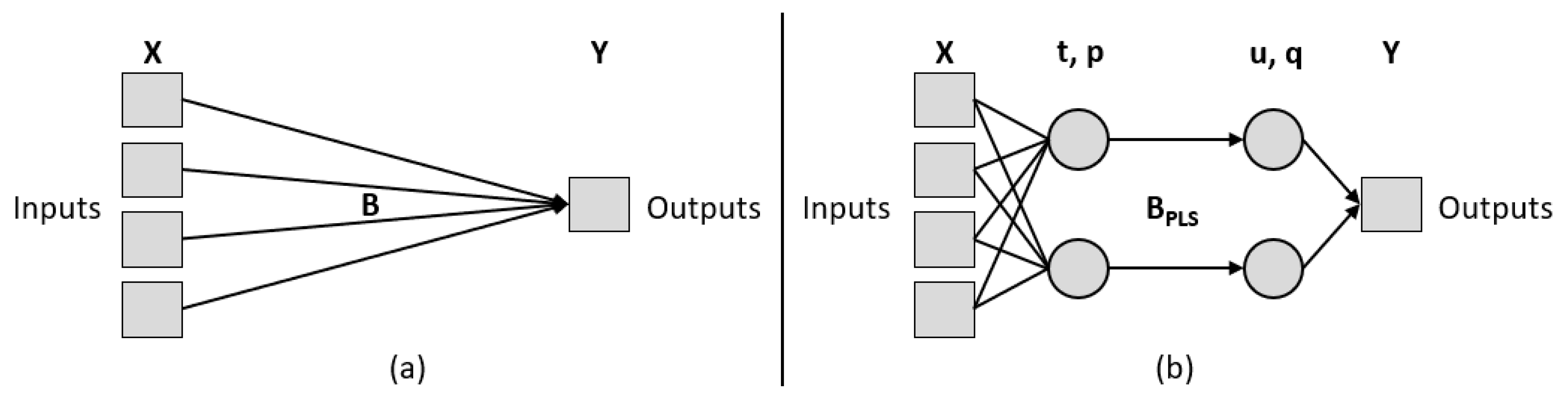
For the predictive modelling portion of the study, elemental, mineralogical and ore composition data, coupled with depositional type, were retained for a total of 46 independent (explanatory) variables including 5 composite variables, e.g., total clays. The depositional setting variable was one-hot encoded to map its categorical data to integer values, represented as a binary vector [74]. Total bitumen recovery was reserved as the lone dependent (response) variable for the sake of this conceptual study. 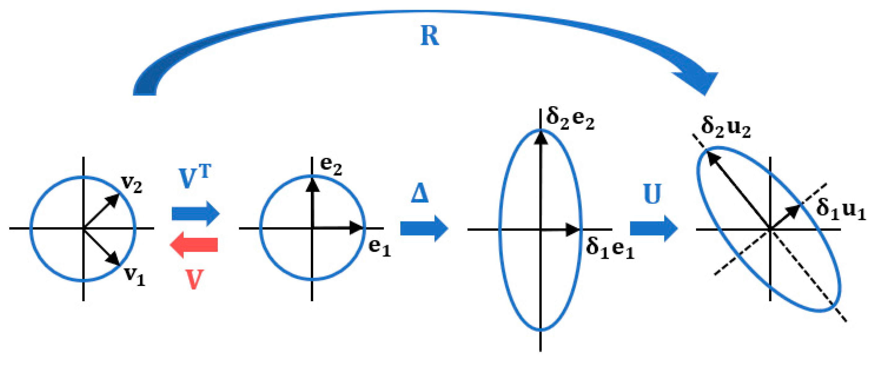A PLS regression algorithm was written in Python coding and follows well-established theory after several authors [43,75,76]. The methodology begins by calculating the SVD of the correlation matrix $R$, as described for Equations (1) and (2), and iteratively computing sets of orthogonal latent variables with the corresponding regression weights.

During each successive iteration, the first left and right singular vectors ($w_l$ and $c_l$) are used as weight vectors to calculate sets of scores ($t_l=X{w}_l$ and $u_l=Y{c}_l$) for $X$ and $Y$, respectively; loadings are then obtained by regressing $X$ and $Y$ against the same vector $t_l$ ($p_l=X^T{t}_l$ and $q_l=Y^T{t}_l$) [75]. The last step of the iteration “deflates” the current data matrices (i.e., removes information related to the $l$th latent variable) by subtracting the outer products $t{p}^T$ and $t{q}^T$ from $X$ and $Y$, respectively [75]. The next component (or latent variable) can then be calculated starting from the SVD of the cross-product of the newly deflated matrices ($X_{l+1}$ and $Y_{l+1}$). The process continues until $X$ is completely decomposed into $L$ components and a null matrix is obtained. After each iteration, vectors $w_l$, $t_l$, $p_l$ and $q_l$ are stored as columns in their respective matrices $W$, $T$, $P$ and $Q$. The matrix of regression coefficients ($B_{PLS}$) can then be calculated as:

$$B_{PLS}=P{(P^{T}P)}^{-1}{Q}^T$$

(3)

where ${(P^{T}P)}^{-1}$ is in fact the Moore-Penrose pseudoinverse for the generalized case of a non-symmetric matrix [76]. Finally, the matrix of regression coefficients ($B_{PLS}$) is multiplied by the original set of independent variables prior to any deflations (matrix $X_0$) to obtain the predictions of the dependent variables (matrix $\widehat{Y}$) [43]. A number of criteria can be calculated to select the appropriate number of components to keep while limiting loss of significance, evaluate the quality of prediction and validate the model, i.e., cross-validation.

Validation is critical to the development of robust predictive models; the quality of prediction must be assessed, and model significance also determined. A common measure of prediction quality is called the residual estimated sum of squares (RESS) and is calculated as follows:

$$\mathrm{RESS}=|\left| Y-\widehat{Y} \right|{|}^2$$

(4)

where $|| |{|}^2$ is the squared matrix norm and decreases as prediction quality improves [43]. However, RESS alone is not the most useful metric, as it will continue to decrease until all components are added, i.e., it does not detect overfitting. An improved measure for quality of prediction is the predicted residual estimated sum of squares (PRESS), computed as follows:

$$\mathrm{PRESS}=|\left| Y-\tilde{Y} \right|{|}^2$$

(5)

where $\tilde{Y}$ represents a predicted set of values generated from cross-validation and also decreases with increasing prediction quality [43]. The selection of the optimal number of components to extract is crucial to avoid overfitting the data. Since prediction quality typically first increases then decreases upon successive component addition, a possible approach is to begin with the first component and stop as soon as the PRESS reverses direction [31]. A more intricate method is to compute the ${\mathrm{Q}}^2$ criterion for the $l$th component, as follows:

$${\mathrm{Q}}_l^2=1-\frac{{\mathrm{PRESS}}_l}{{\mathrm{RESS}}_{l-1}}$$

(6)

and compare against an arbitrary critical value (e.g., $1-{0.95}^2=0.0975$); only components with a ${\mathrm{Q}}_l^2$ value greater than or equal to this threshold are generally kept in the model [31,33].

Because the available dataset is limited to only 60 samples, it was decided not to split the data into separate training and validation sets; instead, leave-one-out cross-validation (LOOCV), also called the “jackknife” method, was utilized. In this technique, each observation is iteratively dropped from the set, and the remaining observations then comprise a training set used to estimate the left-out observation. All estimated observations are stored in a final matrix denoted $\tilde{Y}$, which then serves as the validation set for subsequent prediction quality metrics (e.g., PRESS and ${\mathrm{Q}}^2$ criteria) [31].

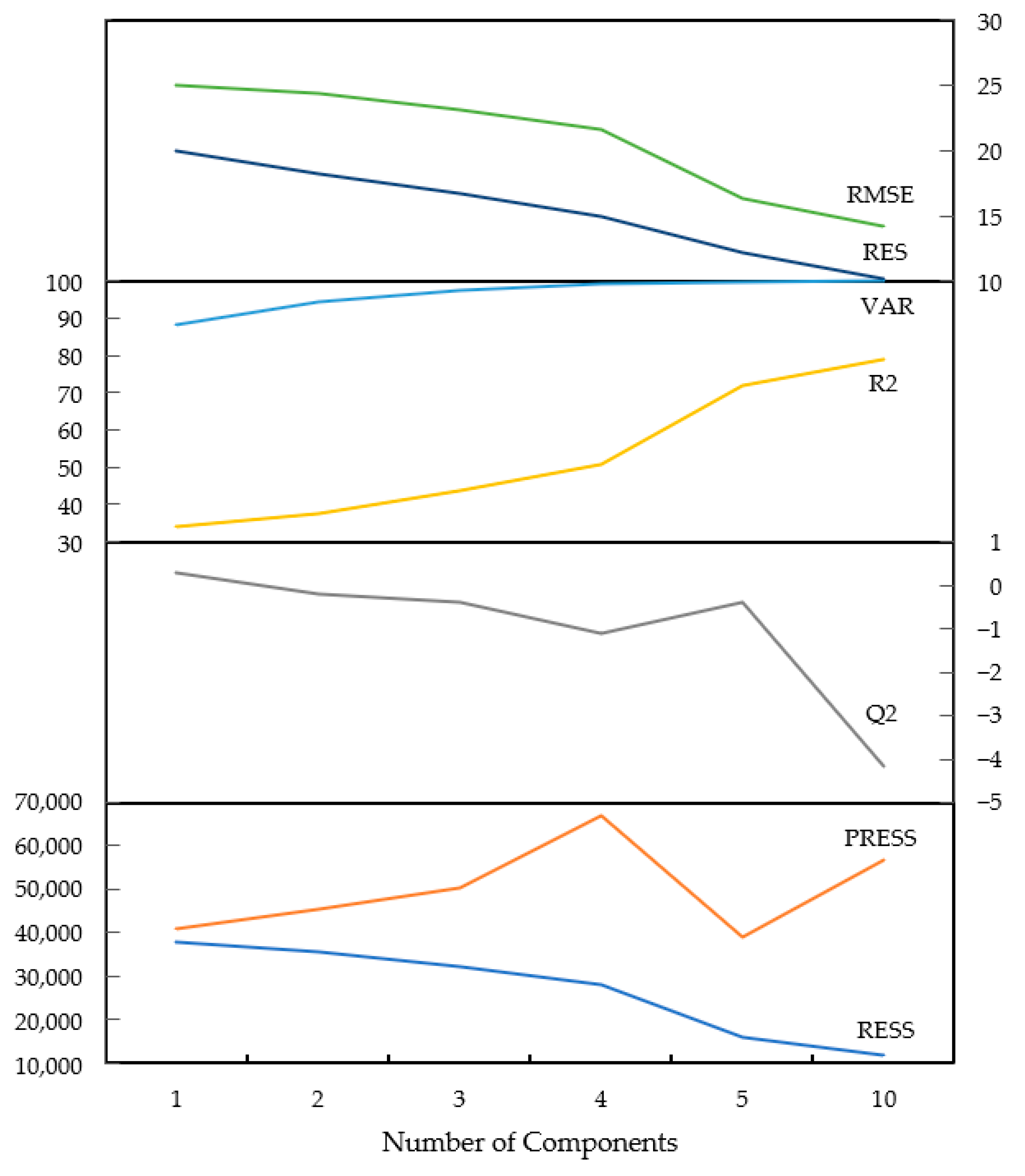
The PLS regression model was run sequentially, and a series of quality of prediction statistics were tabulated for each of 1, 2, 3, 4, 5 and 10 component scenarios (Figure 6). The ${\mathrm{Q}}^2$ criterion indicates that only the first component should be kept in the prediction model, with a value of 0.28, as all ensuing trials resulted in values less than zero. However, not only was the coefficient of determination (R²) quite low for the 1 component scenario (0.34), but root mean squared error (RMSE) and mean absolute residual values were also relatively high. Furthermore, the first component alone only accounts for ~88% of the total model variance, as determined by the sum of squares of the singular values. As a result, the behaviour of the PRESS statistic was tracked upon successive trials in order to identify an improved fit; ultimately, a total of 5 components was deemed appropriate for building the regression model in relation to the available dataset. This was based upon the fact that the PRESS value trended upwards over the first 4 components but dropped significantly upon addition of the fifth; this reversal also coincided with a much higher R² score of 0.72, improved (decreased) RMSE and residual values and an explained variance of 99.65%. Further addition of successive components (e.g., 10 components) did not greatly improve prediction accuracy or error metrics, resulted in poorer PRESS and ${\mathrm{Q}}^2$ statistics and would likely lead to severe overfitting to the present dataset. It is also noteworthy that residuals were consistently greater for marine samples, which indicates greater variability in the predicted set for this depositional type (as expected).

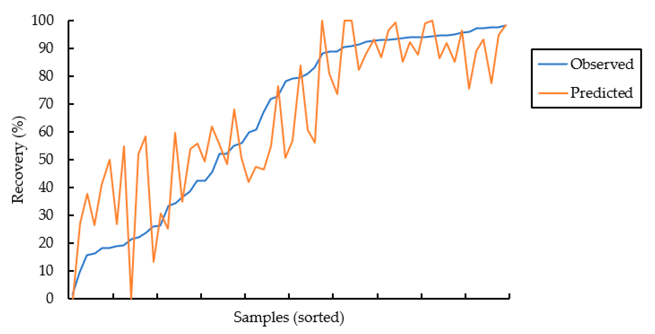
Predictions from the final 5-component model are shown in Figure 7, and comparative descriptive statistics for the observed and predicted datasets are shown in

Table 3. Comparison of summary statistics for observed and predicted bitumen recoveries from PLS regression model (5 components).

Metric	Observed Values (Y)	Predicted Values (Ŷ)
Max (%)	98.29	100.00
Min (%)	1.55	0.00
Median (%)	78.80	61.27
Mean (%)	64.91	65.17
Standard Deviation (%)	31.14	26.91
Variance (%2)	969.95	724.18

. Estimated bitumen recoveries were capped at 100%, and negative values were set to zero, as crossing these thresholds is impossible in practice. The predicted values are generally quite reasonable, within ~11% for the (fluvio-)estuarine samples and ~13% for marine samples on average. This level of error (RMSE of 16.33) is not surprising on account of the assumptions made to finalize the original dataset, in addition to the significant geological variability inherent to oil sands deposits. As expected, the variability in marine sample residuals (standard deviation of 9.89%) is nearly double that of estuarine samples (standard deviation of 5.27%) and can likely be attributed to heterogeneities in clay contents and especially clay types. Overall, the PLS regression model has performed as intended and with a mere total of 60 samples from unknown and/or different mining projects altogether. This highlights the importance of rigorous sampling campaigns and characterization of appropriate geometallurgical profiles towards the development of robust predictive models, particularly for complex operations dealing with multiple and/or heterogeneous ore feeds. It is postulated that the predictive power of the present model would be greatly increased with these controls in place.

Once the regression model has been finalized with the appropriate number of components, confidence intervals for the predicted values can be calculated using the “bootstrap” cross-validation method. This technique involves the random re-sampling of the original observations with replacement, i.e., each observation can be selected zero or multiple times [43]. This is repeated many times (e.g., 1000 or 10,000), and regression coefficients and corresponding predictions are computed for each bootstrapped sample set. The distribution of predicted values from all of these iterations is then used to estimate confidence limits for each variable; intervals that do not span zero (positive or negative) are considered significant [43]. Similarly, bootstrap ratios can be calculated by dividing the mean of each distribution by its standard deviation; akin to a student t-test, if the ratio is greater than a critical value (e.g., >2, corresponding to an alpha value of approximately 0.05), the variable is also considered significant [43].

Table 4. Summary of statistics from 10,000 replications of the bootstrap cross-validation method.

	Independent (Explanatory) Variables
Variable	No. of Observations	Mean (wt.%)	Standard Deviation (wt.%)	Bootstrap Ratio	Lower CI (95%)	Upper CI (95%)
Sample type	60,000	0.57	0.22	2.54	0.20	1.00
Na *	60,000	0.08	0.05	1.57	0.03	0.21
K	60,000	0.64	0.13	5.12	0.45	0.95
Si	60,000	37.97	0.96	39.70	35.30	39.42
Al	60,000	2.22	0.64	3.48	1.34	3.99
Fe	60,000	0.72	0.24	2.98	0.35	1.42
Mg *	60,000	0.12	0.10	1.19	0.02	0.48
Ca *	60,000	0.30	0.31	0.99	−0.02	1.53
Ti	60,000	0.25	0.06	3.95	0.15	0.38
Zr	60,000	0.04	0.02	2.41	0.01	0.08
P	60,000	0.02	0.01	2.40	0.01	0.04
C	60,000	7.87	1.00	7.90	5.88	9.67
S	60,000	0.47	0.13	3.64	0.25	0.76
Bitumen	60,000	8.79	1.36	6.46	6.06	11.16
Water	60,000	6.64	1.42	4.69	4.25	9.97
Solids	60,000	84.42	1.11	76.29	82.27	86.83
Fines	60,000	34.27	7.91	4.33	22.22	52.30
Quartz + silica	60,000	74.94	3.46	21.64	64.62	79.82
Illite	60,000	5.89	1.66	3.55	3.43	10.21
Kaolinite	60,000	3.90	1.83	2.13	1.08	8.58
Chlorite *	60,000	0.10	0.14	0.73	−0.16	0.41
Calcite (Cal) *	60,000	0.09	0.28	0.33	−0.24	1.07
Dolomite (Dol) *	60,000	0.84	0.82	1.01	−0.03	3.67
Ankerite (Ank) *	60,000	0.06	0.07	0.85	−0.05	0.21
Siderite (Sid)	60,000	1.04	0.50	2.07	0.10	2.19
Pyrite *	60,000	0.16	0.11	1.40	−0.02	0.46
Zircon	60,000	0.09	0.04	2.41	0.02	0.17
Rutile (Rut)	60,000	0.15	0.04	3.73	0.07	0.22
Anatase (Ana)	60,000	0.26	0.10	2.64	0.12	0.49
Ilmenite	60,000	0.02	0.00	3.74	0.01	0.03
Lepidolite	60,000	0.02	0.00	3.72	0.01	0.03
Gypsum *	60,000	0.01	0.06	0.19	−0.12	0.11
Bassanite *	60,000	0.01	0.06	0.16	−0.13	0.10
Anorthite (Ano) *	60,000	0.22	0.61	0.36	−0.92	1.77
K-feldspar (Ksp)	60,000	1.20	0.38	3.17	0.39	1.96
Albite (Alb) *	60,000	0.96	0.61	1.57	0.29	2.36
Iron oxide/hydroxide (AFE) *	60,000	0.19	0.44	0.42	−0.46	1.55
Apatite	60,000	0.09	0.04	2.34	0.04	0.22
Cristobalite	60,000	0.01	0.00	2.70	0.00	0.02
Organic carbon	60,000	7.63	1.00	7.63	5.61	9.41
Organic sulphur	60,000	0.39	0.13	2.96	0.14	0.67
Total clays	60,000	9.89	3.24	3.05	5.13	19.00
Sid + AFE	60,000	1.22	0.49	2.48	0.45	2.52
Rut + Ana	60,000	0.40	0.11	3.82	0.24	0.63
Cal + Dol + Ank *	60,000	0.98	1.01	0.97	−0.05	4.39
Ano + Ksp + Alb	60,000	2.37	0.82	2.91	1.09	4.76
	Dependent (response) variables
Variable	No. of observations	Mean (wt.%)	Standard deviation (wt.%)	Bootstrap ratio	Lower CI (95%)	Upper CI (95%)
Total Recovery	60,000	64.84	28.86	2.25	1.52	109.53

* Insignificant variables determined from the distribution of 10,000 bootstrap sample sets.

provides statistics computed from the distribution of 10,000 bootstrap sample sets generated from the 5-component regression model; variable significance was determined based on both bootstrap ratios and 95% confidence intervals. Of the elemental composition variables, only Na, Ca and Mg were deemed insignificant. Corresponding insignificant minerals include albite for Na; gypsum, bassanite and anorthite for Ca; chlorite for Mg; the carbonates (calcite, dolomite and ankerite) for both Ca and Mg. Interestingly, both pyrite and amorphous Fe-oxides/hydroxides were also considered insignificant (oil sands tend to contain significant heavy metals). All remaining elements and mineral phases, in addition to depositional sample type and bitumen recovery, were determined as statistically significant.

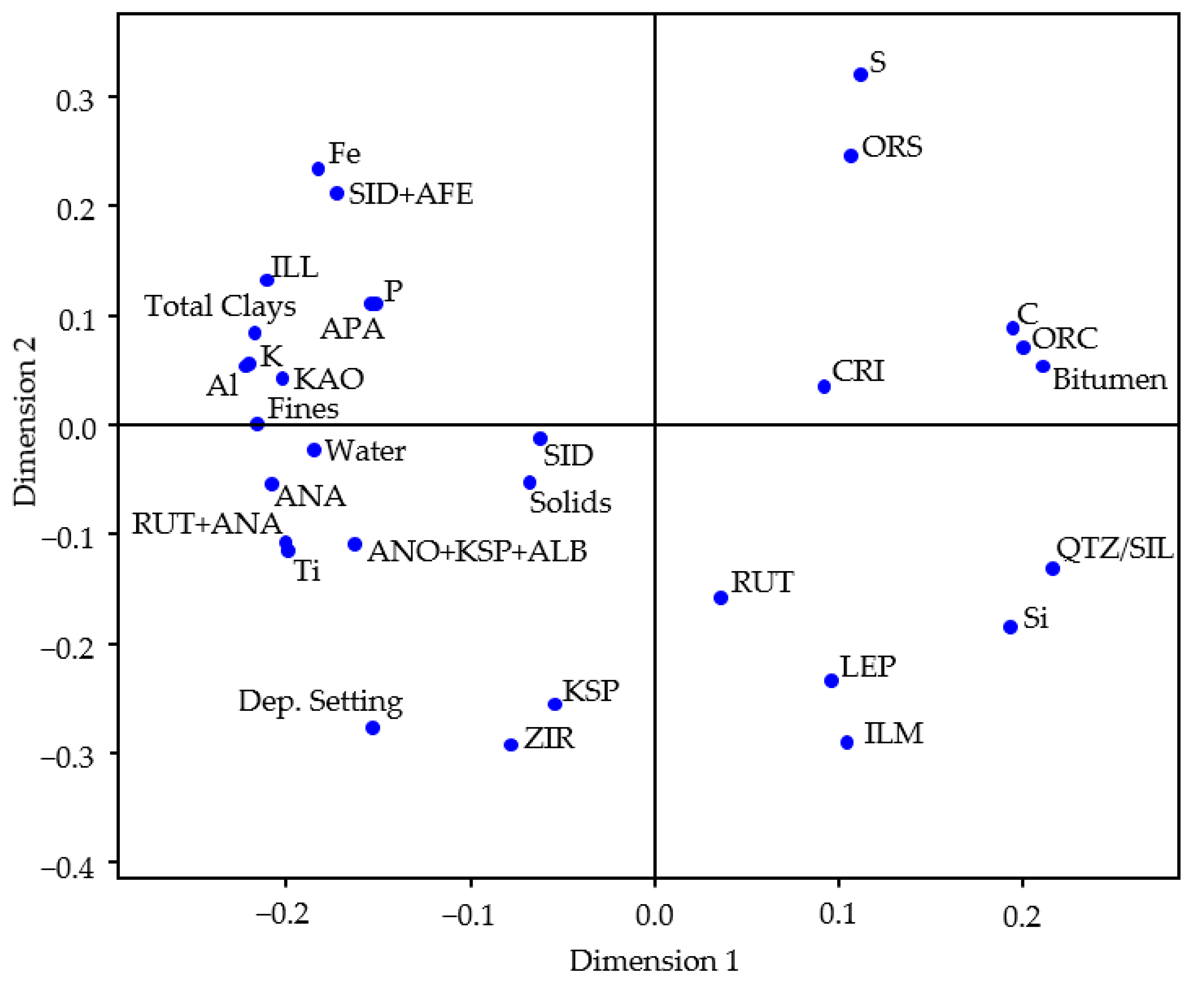
The relationships between the independent variables can be observed visually by plotting the stored $X$-loadings (matrix $P$) for the first two components (Figure 8). Bitumen content is clearly most strongly linked to elemental carbon and organic carbon (as expected); it also appears in association to silicon (quartz–silica–cristobalite), sulphur (organic sulphur), titanium minerals (rutile and ilmenite) and lepidolite (Li-rich mica). The first dimension also opposes the bitumen group from the clay minerals, water content and carbonates (siderite). Notably, anatase (metastable form of TiO₂) plots opposite the other Ti-bearing phases. In the second dimension, the organic-related groups (bitumen, carbon and sulphur) clearly oppose the related silicate and oxide minerals; there is also a broad separation between silicates and carbonate + iron-bearing phases.

Overall, the PLS regression model has proven to be a powerful prediction tool, capable of providing additional useful information regarding process variables that can help drive the characterization of geometallurgical profiles, sampling methodologies and other planning processes.

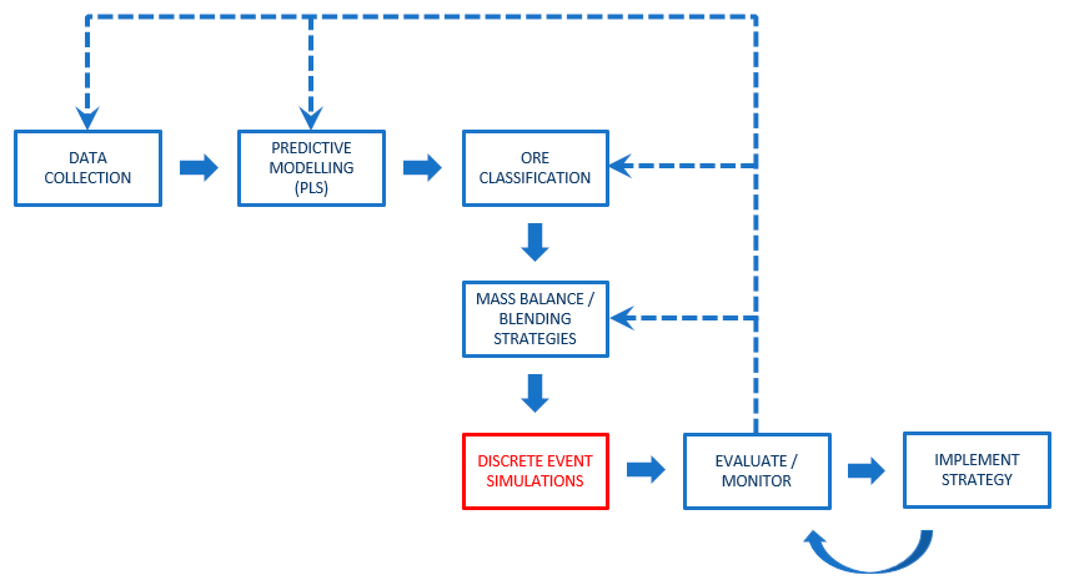
3.2.2. Discrete Event Simulations

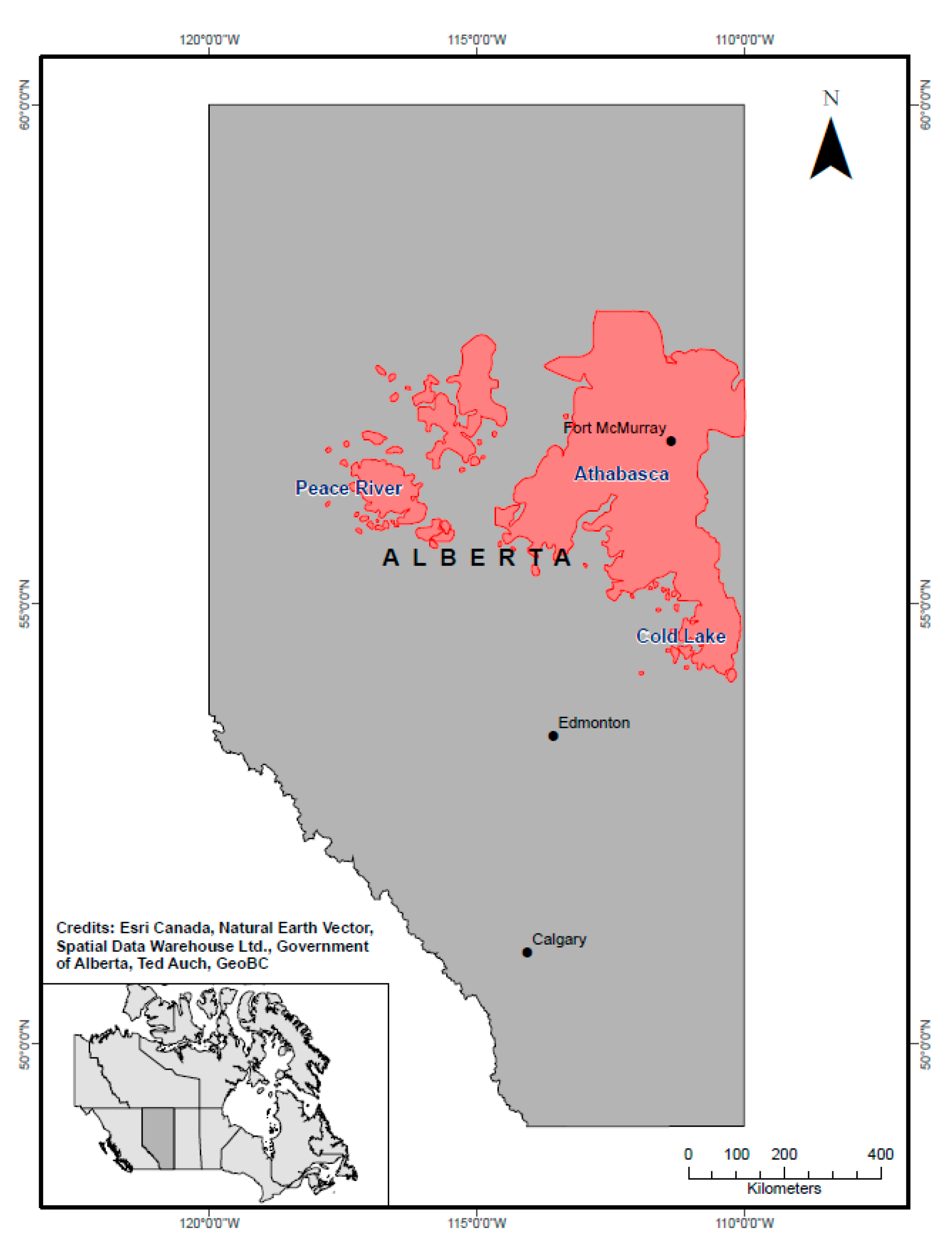
For the DES portion of the study, two ore types were classified according to documented depositional setting and predicted bitumen recoveries from the 5-component PLS regression model. Ore type 1 consists entirely of marine samples (generally <75% recovery), and ore type 2 includes (fluvio-)estuarine samples (>75% recovery) as well as a few of marine type with recoveries also greater than 75%. Due to the limited nature of the dataset (only 3 samples per mining parcel), natural background noise was added to the relative proportions of ore types 1 and 2 via random number generation with a standard deviation of 5%. Two modes of operation (A and B) are considered here to balance stockpile levels against bitumen extraction rates and incoming ore feed from mining. While the conceptual mine has been operating in areas predominantly containing ore type 2 (favourable due to higher grades and recoveries) for some time, a large expansion of reserves comprising mainly ore type 1 has recently been completed. With the expansion, longer term forecasts suggest an overall deposit composition of 55–45% for ore types 1 and 2, respectively, with increased variability caused by geological heterogeneities; these values correspond to the average proportions determined from ore classification based on the predictive modelling.

In order to sustain the availability of ore type 2 and improve the economics of certain portions of the newly expanded area, the operation is evaluating possible adjustments to current blending strategies and intends to implement a secondary alternate mode. Based on the geological attributes of ore types 1 (high bitumen, low fines) and 2 (high fines), the new strategy will also serve to control the distribution of solids in ore feeds to the froth treatment plant, thereby improving amenability to transport via pipelines to the upgrader. As a result, operational Mode A will consist of an approximate 40–60 blend of ores 1 and 2. Because ore type 2 will generally be in shorter supply, a second operational Mode B, consisting of an 80–20 blend of ores 1 and 2, is needed in order to avoid stockouts, or an eventual shortage. This will ultimately stabilize feed balances, maximize equipment/infrastructure selection and utilization and allow for improved production scheduling; collectively, these factors can lead to significant reductions in operating and capital costs.

Both modes are expected to perform similarly in terms of downstream bitumen recovery processes, except that Mode B requires a pre-treatment stage to control excess chloride ions related to the marine origin and high fines content of ore type 1. Consequently, bitumen extraction rates for Mode B are set 10% lower than those for Mode A; modal parameters for each configuration are summarized in

Table 5. Description of operational modes in relation to deposit forecast.

		Throughput (t/h)	Ore 1 in Feed (%)	Ore 2 in Feed (%)
Algebraic Notation:		rA,ACont,B,BCont	w1A,1ACont,1B,1BCont	w2A,2ACont,2B,2BCont
Mode A	Regular	30,000	40	60
	Contingency	19,500	100	0
Mode B	Regular	27,000	80	20
	Contingency	13,500	0	100
Deposit		-	55	45

. Despite the fact that Mode A is both more productive and economical, ore stockouts would be inevitable over extended periods of usage because the weight fraction of ore type 2 (w_2A) is 15% higher than that of the deposit (w_2D). To account for the possibility of stockouts prior to a planned shutdown, contingency modes with adjusted configuration rates have been incorporated for each of Modes A and B.

Appropriate weight fractions (w_1A,2A,1B,2B) and throughput rates (r_A,B) are assessed with respect to geological estimations (w_1D,2D) using deterministic mass balancing, as follows [15,17]:

$$\left(\frac{t_{\mathrm{A}}}{t_{\mathrm{B}}}\right)=\left(\frac{w_{2\mathrm{B}}{w}_{1\mathrm{D}}-w_{1\mathrm{B}}{w}_{2\mathrm{D}}}{-w_{2\mathrm{A}}{w}_{1\mathrm{D}}+w_{1\mathrm{A}}{w}_{2\mathrm{D}}}\right)\left(\frac{r_{\mathrm{B}}}{r_{\mathrm{A}}}\right)$$

(7)

where t_A and t_B denote the time elapsed under Modes A and B, respectively. Average throughput between the two modes, or similarly between each mode and its corresponding contingency configuration, can then be computed as follows [15,17]:

$$r=\left(\frac{w_{1\mathrm{A}}{w}_{2\mathrm{B} }-w_{2\mathrm{A}}{w}_{1\mathrm{B}}}{\left(w_{2\mathrm{B}}\left(\frac{r_{\mathrm{B}}}{r_{\mathrm{A}}}\right)-w_{2\mathrm{A}}\right)w_{1\mathrm{D} }-\left(w_{1\mathrm{B}}\left(\frac{r_{\mathrm{B}}}{r_{\mathrm{A}}}\right)-w_{1\mathrm{A}}\right)w_{2\mathrm{D}}}\right)r_{\mathrm{B}}$$

(8)

Equations (7) and (8), which ignore the risk of stockout, indicate that Mode A should be applied 1.5 times as often as Mode B, with an average throughput of 28,800 t/h. The framework aims to simultaneously maximize throughput and minimize target stockpile levels, thereby increasing production efficiency and reducing overall costs; larger stockpiles necessitate larger storage areas and equipment, as well as increased handling costs.

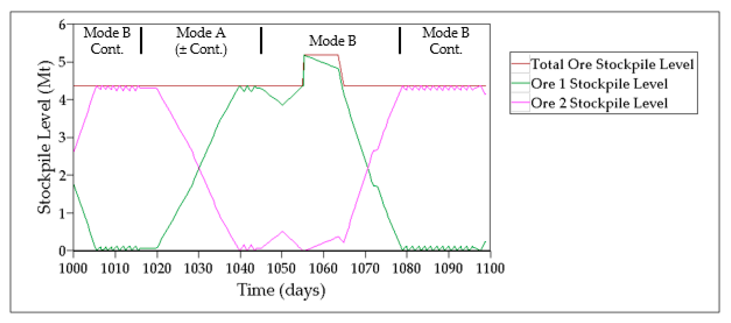
The current framework is designed such that mining rates exceed plant capacity, hence the plant acts as a bottleneck. To ensure stockpiles are adequately supplied to maintain consistent ore feed to the plant, ore will be mined at minimum rates of 30 kt/h under Mode A and 27 kt/h under Mode B. Target total stockpile level is a control variable that remains constant (except during extended stockout periods); however, the relative proportions of ore types 1 and 2 fluctuate contingent on the active operational mode. Mode A (productive phase) causes a relative decrease in the proportion of ore type 2, meanwhile Mode B (replenishment phase) has the opposite effect. The selection of operational mode is based on the stockpile level of the limiting ore type (in this case, ore 2) at the end of a production campaign during planned shutdowns every 4 weeks.

Under the present framework (Table 5), a naïve analysis indicates a critical threshold of 2.916 Mt for ore type 2; this level is computed as a function of campaign length (27 days) and rate of change under Mode A (108,000 t/d; plant capacity of 720,000 t/d × w_2D of 45% less relative critical ore 2 throughput from 40–60 blending strategy). Similarly, the analysis indicates a minimum total target stockpile level (sum of ores 1 and 2) of 4.374 Mt, determined as the maximum rate of change between ore stockpiles 1 and 2 as a function of campaign duration (under either mode). However, the digital twin is subject to the geological uncertainty of the ore, which is not taken into account by Equations (7) and (8). Unexpected fluctuations in ore feed attributes can indeed cause either overages or shortfalls for a given ore type, potentially leading to stockout towards the end of a production campaign [15]. To mitigate this risk, an operational buffer can be introduced by raising the threshold for the critical (limiting) ore type; a similar control measure would be to raise the target total stockpile level.

Because stockouts are nonetheless a real possibility, recourse actions are built into the digital twin to maintain ore feed consistency. These recourse actions depend on the timing of stockout; if an ore type is depleted during a production campaign, a contingency mode is enacted that allows the exhausted stockpile to build back up. As indicated in Table 5, Contingency Mode A only consumes ore type 1, and Contingency Mode B only consumes ore type 2. These contingency modes are much less productive than the regular configuration rates (65% for Mode A and 50% for Mode B); as a result, the duration of these segments has been limited to 1 day, which causes alternations until the next planned shutdown. If the critical ore level remains below the selected threshold at the end of a campaign, the plant will employ the alternate mode of operation to re-equilibrate stockpile levels. Time segment parameters for production campaigns, shutdowns and contingency mode duration are summarized in

Table 6. Summary of time segment parameters.

Segment Type	Duration (Days)
Production campaign	27
Planned shutdown	1
Contingency modes	1
Regular modes	Indeterminate

.

The current framework was implemented, and subsequent computational results (

Table 7. Distribution of time spent in each mode type under varied target total stockpile levels.

Scenario:		1	2	3		4	5
Replications:		1	1	1	100	1	1
Critical Ore 2 Level (Mt):		2.916	2.916	2.916	2.916	2.916	2.916
Target Total Stockpile Level (Mt):		4.374 (1×)	6.561 (1.5×)	8.748 (2×)	8.748 (2×)	13.122 (3×)	21.870 (5×)
		Portion of time (%)
Mode A	Regular	45.6	54.8	59.7	60.1	58.4	59.4
	Contingency	4.9	0.2	1.6	1.4	0.6	0.6
Mode B	Regular	34.8	37.3	35	34.5	37.4	36.4
	Contingency	11.1	4.2	0.1	0.4	0	0
Shutdown		3.6	3.5	3.6	3.6	3.6	3.6
Throughput (kt/h)		26.5	28.1	28.7	28.7	28.8	28.8
Replications with stockouts		-	-	-	82	-	-

and

Table 8. Distribution of time spent in each mode type under varied critical ore levels.

Scenario:		6		7		8
Replications:		1	100	1	100	1	100
Critical Ore 2 Level (Mt):		5.832 (2×)	5.832 (2×)	7.290 (2.5×)	7.290 (2.5×)	8.748 (3×)	8.748 (3×)
Target Total Stockpile Level (Mt):		11.664	11.664	14.580	14.580	17.496	17.496
Mode A	Regular	58.7	59.6	58.6	60.0	58.6	60
	Contingency	0	0.1	0	0.05	0	0
Mode B	Regular	37.3	36.3	37.8	36.3	37.8	36.4
	Contingency	0.4	0.4	0	0.05	0	0
Shutdown		3.6	3.6	3.6	3.6	3.6	3.6
Throughput (kt/h)		28.8	28.8	28.8	28.9	28.8	28.9
Replications with stockouts		-	62	-	5	-	0

, Figure 9 and Figure 10) generated, using commercial DES software (Rockwell Arena©) with Visual Basic for Applications (VBA). Extended operating periods can be simulated to assess system performance in response to geological uncertainty, with adjustments made to the critical ore and target stockpile levels as control variables. In its present configuration, the simulation model assumes that ore is mined to completion from a single parcel at a time. The framework has the flexibility to incorporate geological uncertainty by reading data from external source files. For the purposes of this study, uncertainty was introduced through Monte Carlo simulation; the proportions of ore types 1 and 2, determined from the classification of mining parcels based on depositional setting and predicted recoveries, were used to generate 100 statistical replicas through random number generation with a standard deviation of 5%. The model is configured such that 792 Mt of ore are processed within each replica, corresponding to approximately 1200 days of operation.

A series of simulations were run to observe the effects of the selected control variable levels on throughput and potential stockout risk, in response to geological uncertainty. The first set of trials varied the total stockpile target levels, while holding the critical ore 2 level constant at 2.916 Mt (deterministic value). A total of 5 scenarios were considered with total stockpile levels set at 1× (“one times”), 1.5×, 2×, 3× and 5× the deterministic value (4.374 Mt); simulated results for each are summarized in Table 7.

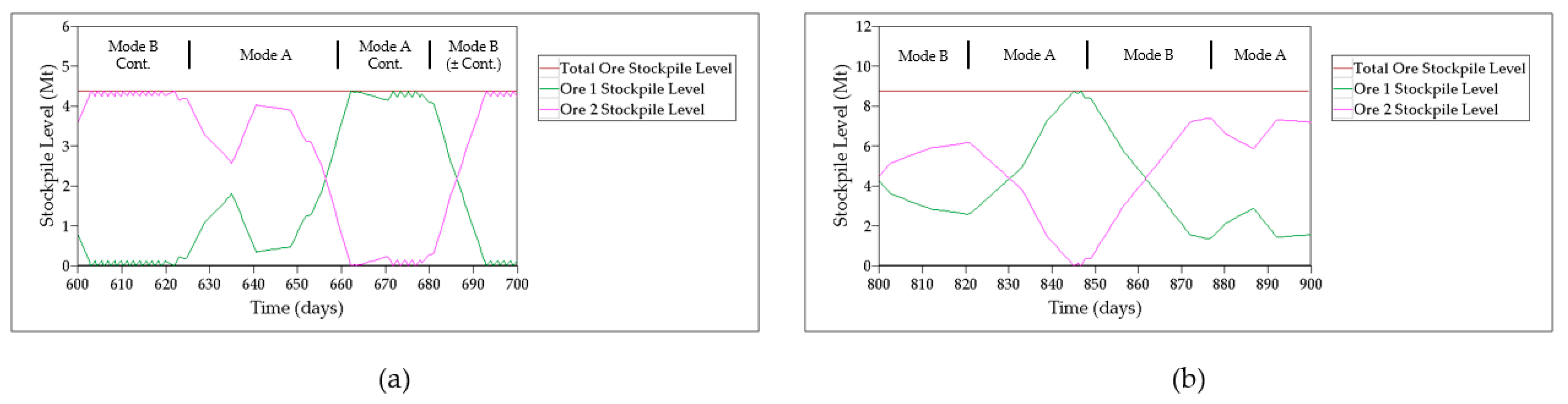
Consistent with Navarra et al. [15] and Wilson et al. [17], the results show that naïve selection of the total stockpile target level does not perform well over extended operating periods, with Mode A being applied only 1.1× as often as Mode B for an average throughput of 26.5 kt/h. This is clearly less productive than the deterministic result of 28.8 kt/h (Mode A applied 1.5× more than Mode B), and the simulated operation also suffered from frequent sustained shortages of both ore types (Figure 9a). Increasing the total stockpile level by just 1.5× (Scenario 2) already improves overall system response; however, with Mode A applied 1.3× as often as Mode B for an average throughput of 28.1 kt/h, this is still worse than expected from Equations (7) and (8). Scenario 3, which doubled the deterministic total stockpile level to 8.748 Mt, produced the best overall results with Mode A applied 1.75× more frequently than Mode B for an average throughput of 28.7 kt/h; there was also a drastic reduction in the proportion of time spent in contingency modes (Figure 9b). Successive increases to the stockpile targets (Scenarios 4 and 5) did not show any marked changes, and system performance was actually slightly worse for both. These results suggest that in order to maximize throughput and mitigate stockout risk, the target total stockpile level is best maintained in the range of 2–3 times the selected critical ore threshold.

Using the parameter values established from Scenario 3, the framework was subsequently configured to simulate 100 replications, corresponding to approximately 120,000 days of operation. Average results from this test mirrored those of the single replication (Table 7) but highlighted repeated ore shortages as a significant operating risk under this scheme, with 82% of the replications confronted by stockouts. While not apparent from the single replication simulation, this outcome is directly related to the high variability of the dataset and is entirely possible in the context of oil sands mining, particularly when dealing with multiple and/or heterogeneous ore feed sources. Frequent and/or sustained stockout periods (especially early in a campaign) require additional consideration; as a recourse action, the possibility for mining surges has been incorporated into the framework in order to supply ore feed directly to the plant to maintain production (Figure 10).

To attenuate the significant stockout risk observed under Scenario 3, a second set of simulations were executed in which adjustments were made to the critical ore limit while keeping the total stockpile target at 2× this level. Four scenarios were tested with critical ore levels designated at 1.5×, 2×, 2.5× and 3× the deterministic value (2.916 Mt); results for each simulation trial are summarized in Table 8. While variations in the critical ore threshold had no meaningful effect on throughput rates or modal proportions, important reductions in the number and frequency of stockout periods were observed with the framework configured for 100 replications (~120,000 operating days). At twice the deterministic value (Scenario 6), the number of replications affected by ore shortages was reduced by 20% (cf. Scenario 3); at 2.5× (Scenario 7), this number decreased to just 5%. Tripling the critical value actually eliminated simulated stockout periods altogether; however, increased capital and operating costs associated with exceedingly large stockpile levels must be weighed against the risk of stockout in the decision-making process.

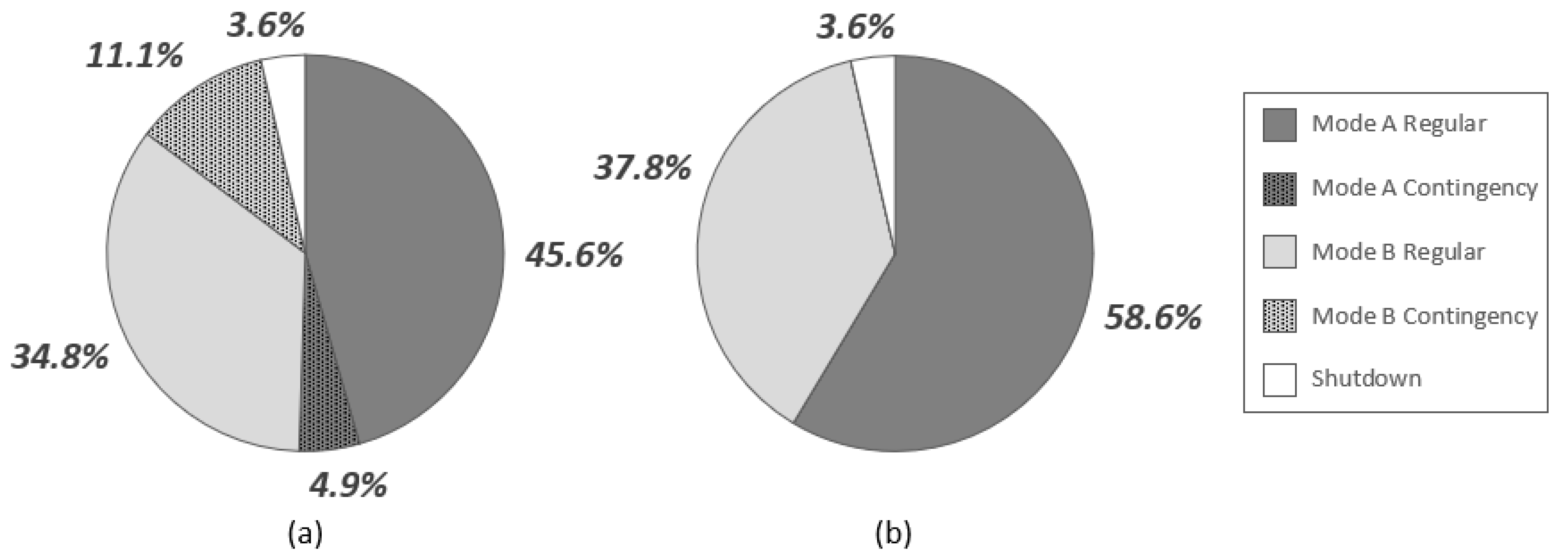
The time-averaged distribution of operational modes in response to geological uncertainty can be useful to evaluate the effects of varied control parameters. Figure 11a represents the naïve approach of Scenario 1, in which the deterministic values for the critical ore level (2.916 Mt) and total stockpile target level (4.374 Mt) were applied; Figure 11b depicts the enhanced framework configuration established under Scenario 7 (described above). The latter scheme is a significant improvement over the naïve setup, with an 8–9% increase in the proportion of time spent under Mode A, a much lower reliance on contingency modes (~15%) and the virtual elimination of ore stockouts. All of these factors contribute to improved production efficiencies; moreover, the enhanced configuration is also more economical based on higher consumption rates for ore type 2, which boasts higher overall grades and bitumen recoveries. Both framework applications benefit from the ability to switch between modes relatively freely in response to data variability, but the enhanced configuration is much less susceptible to operational risk caused by geological heterogeneities.

Overall, these simulation results support the flexibility of DES digital twins to integrate predictive modelling data generated through PLS regression (or other advanced methods) in order to assess the system-wide response to geological uncertainty. This quantitative framework is an extension of recent conceptual work by Navarra et al. (2019) and Wilson et al. (2021) and demonstrates its adaptation to evaluate operational risk factors associated with potential processing applications for Canada’s oil sands. Simulations indicate that ore stockouts are a very real possibility due to extreme geological heterogeneities inherent to oil sands; however, the current digital twin allows for the analysis of potential adjustments to control strategies at an earlier stage, which can help drive decision making and mitigate identified risk factors. The blending control strategies described in this study would necessitate significant stockpiling infrastructure and equipment, but these implied costs could easily be offset by higher throughputs, minimized downtime and extended operational life achieved through the implementation of alternate modes of operation.

4. Discussion and Future Work

Geological variability and related uncertainty are inherent to all ore deposit types. These heterogeneities can range in intensity and generally vary both within and between deposits and/or mining districts. This can lead to unexpected changes in ore feed attributes (e.g., grade, mineralogy, grain size distribution), thereby affecting the mining and extractive processes. All of these factors have a direct impact on the interplay of critical variables and integrated coordination of processes within the overall system. Given that ore feeds are exploited from complex and heterogeneous sources, it is clear that mining systems need to be flexible, with the ability to respond to changes and communicate with all related processes (both up and downstream). The availability of alternate operational modes, each with its own set of instructions, is crucial to the sustained development of most orebodies, particularly as a project matures and evolves.

The implementation of operational buffers and other control strategies is not uncommon, but the development of suitable tools that incorporate predictive models to enhance or optimize system processes is lagging behind. Efforts are sometimes made to capture detailed information but then is not properly integrated into actual system process controls due to interdisciplinary barriers. The current study focused on ore blending strategies and overall feed management through the integration of predictive PLS regression models into a DES framework within an oil sands context. The results confirm the approach as an effective way to improve and stabilize plant throughput, despite challenges with significant geological variation of source ore feeds inherent to Canada’s oil sands. Despite a small sample population and incomplete characterization (i.e., minimal depositional provenance and bitumen recovery data), the integrated quantitative framework made reasonable predictions and demonstrated how appropriate mineral and geochemical characterization could positively impact process control strategies and decision making earlier in the value chain.

As ore compositional data are routinely collected in the industry via the Soxhlet-Dean and Stark method, bitumen free solids (BFS) are readily available for geochemical and/or mineralogical analyses that can be used for predictive modelling. This work proposes that, with adequate sampling and characterization, expensive and time-consuming analytical work (e.g., organic-rich solids separation) can be replaced by faster and cheaper alternatives, such as WD-XRF and XRD executed on BFS streams [66]. The generation of robust predictive models will require extensive systematic sampling and analytical campaigns to properly characterize ore feeds and related downstream process responses; the degree of sampling is difficult to anticipate in advance and ultimately depends on data variability as well as the exact problem being addressed. Regardless, the ability to integrate reliable predictions of bitumen processability into a DES digital twin earlier in the value chain is of key importance to assess the effects of heterogeneous ore feeds on system process performance. Adjustments can then be made to operating practices (e.g., alternate modes of operation or the introduction of operational buffers) in order to mitigate the identified risk factors.

Similar to other complex mining projects, oil sands operations are host to a variety of treatments and processes. From mining to slurry and froth formation, froth treatment, upgrading and pipeline transport (each possibly comprised of multiple sub-systems), there are a large number of moving parts requiring both management and coordination. The interaction of these parts can be a major source of bottlenecks and generate severe deficiencies, which makes the oil sands context an ideal candidate for DES modelling. However, coordinated efforts between academic, government and industry partners are required in order to couple recent advances in quantitative methods with project-specific problems and data; only then can detailed flowsheets, testing and full system optimization with constraints proceed.

This conceptual study makes broad assumptions regarding ore characteristics and recoveries for demonstrative purposes but shows the suitability of the approach for multivariate ore processing systems. In practice, the ability to collect a sufficient level of data for appropriate ore characterization and build robust predictive models is challenging. This work is focused on analyzing operational risk related to oil sands mining and bitumen extraction processes with respect to geological uncertainty; in reality, overall bitumen recovery is not only based on ore characteristics, but also on changes in processing conditions, e.g., temperatures, additives and densities [77]. As such, the extensibility of the framework would allow for the eventual integration of other advanced quantitative methods, such as non-linear machine learning algorithms. The flexibility of DES digital twins to incorporate varying levels of detail makes it particularly well suited to multi-phase (re)engineering projects and can help improve confidence at each stage of development.

References

1. Bata, T.; Schamel, S.; Fustic, M.; Ibatulin, R. AAPG Energy Minerals Division Bitumen and Heavy Oil Committee Annual Commodity Report—May 2019; American Association of Petroleum Geologists (AAPG): Tulsa, OK, USA, 2019. [Google Scholar]
2. Canada Energy Regulator (CER). Canada’s Energy Future 2020: Energy Supply and Demand Projections to 2050 (EF2020); Canada Energy Regulator: Ottawa, ON, Canada, 2020.
3. Hein, F.J. Heavy oil and oil (tar) sands in North America: An overview & summary of contributions. Nat. Resour. Res. 2006, 15, 67–84. [Google Scholar]
4. Gray, M.R.; Xu, Z.; Masliyah, J. Physics in the oil sands of Alberta. Phys. Today. 2009, 62, 31–35. [Google Scholar] [CrossRef]
5. Algeer, R.; Snowdon, L.; Huang, H.; Oldenburg, T.; Larter, S. Is water washing an important petroleum system process? In Proceedings of the AAPG Annual Convention and Exhibition, Calgary, AB, Canada, 19–22 June 2016.
6. Fustic, M.; Ahmed, K.; Brough, S.; Bennett, B.; Bloom, L.; Asgar–Deen, M.; Jokanola, O.; Spencer, R.; Larter, S. Reservoir and bitumen heterogeneity in Athabasca oil sands. AAPG Search Discov. 2015, 20296, 15. [Google Scholar]
7. Masliyah, J.H.; Czarnecki, J.; Xu, Z. Handbook on Theory and Practice of Bitumen Recovery from Athabasca Oil Sands, Volume 1: Theoretical Basis; Kingsley Knowledge Publishing: Cochrane, AB, Canada, 2011. [Google Scholar]
8. Gray, M.R.; Eaton, P.E.; Le, T. Inhibition and promotion of hydrolysis of chloride salts in model crude oil and heavy oil. Pet. Sci. Technol. 2008, 26, 1934–1944. [Google Scholar] [CrossRef]
9. Kaur, H.; Eaton, P.E.; Gray, M.R. The kinetics and inhibition of chloride hydrolysis in Canadian bitumen. Pet. Sci. Technol. 2012, 30, 993–1003. [Google Scholar] [CrossRef]
10. Li, X.; Wu, B.; Zhu, J. Hazards of organic chloride to petroleum processing in Chinese refineries and industrial countermeasures. Progress Petrochem. Sci. 2018, 2, 204–207. [Google Scholar] [CrossRef]
11. Londono, Y.; Mikula, R.; Eaton, P.E.; Gray, M.R. Interaction of chloride salts and kaolin clay in the hydrolysis of emulsified chloride salts at 200–350 C. Pet. Sci. Technol. 2009, 27, 1163–1174. [Google Scholar] [CrossRef]
12. Navarra, A.; Grammatikopoulos, T.; Waters, K. Incorporation of geometallurgical modelling into long–term production planning. Miner. Eng. 2018, 120, 118–126. [Google Scholar] [CrossRef] [Green Version]
13. Navarra, A.; Rafiei, A.; Waters, K. A systems approach to mineral processing based on mathematical programming. Can. Metall. Q. 2017, 56, 35–44. [Google Scholar] [CrossRef]
14. Navarra, A.; Wilson, R.; Parra, R.; Toro, N.; Ross, A.; Nave, J.-C.; Mackey, P.J. Quantitative methods to support data acquisition modernization within copper smelters. Processes 2020, 8, 1478. [Google Scholar] [CrossRef]
15. Navarra, A.; Alvarez, M.; Rojas, K.; Menzies, A.; Pax, R.; Waters, K. Concentrator operational modes in response to geological variation. Miner. Eng. 2019, 134, 356–364. [Google Scholar] [CrossRef]
16. Saldana, M.; Toro, N.; Castillo, J.; Hernandez, P.; Navarra, A. Optimization of the heap leaching process through changes in modes of operation and discrete event simulation. Minerals 2019, 9, 421. [Google Scholar] [CrossRef] [Green Version]
17. Wilson, R.; Toro, N.; Naranjo, O.; Emery, X.; Navarra, A. Integration of geostatistical modeling into discrete event simulation for development of tailings dam retreatment applications. Miner. Eng. 2021, 164, 106814. [Google Scholar] [CrossRef]
18. Boschert, S.; Rosen, R. Digital Twin—The Simulation Aspect. In Mechatronic Futures; Hehenberger, P., Bradley, D., Eds.; Springer International Publishing: Cham, Switzerland, 2016; pp. 59–74. [Google Scholar]
19. Glaessgen, E.H.; Stargel, D.S. The digital twin paradigm for future NASA and U.S. Air Force vehicles. In Proceedings of the 53rd Structures, Structural Dynamics, and Materials Conference: Special Session on the Digital Twin, Honolulu, HI, USA, 23–26 April 2012. [Google Scholar]
20. Kaminsky, H.A.W. Characterization of an Athabasca Oil Sands Ore and Process Streams. PhD Thesis, Department of Chemical and Materials Engineering, University of Alberta, Edmonton, AB, Canada, 2008. [Google Scholar]
21. Energy Resources Conservation Board (ERCB). Alberta’s Energy Reserves 2008 and Supply/Demand Outlook 2009–2018; Energy Resources Conservation Board: Calgary, AB, Canada, 2009.
22. Zhao, S.; Kotlyar, L.S.; Sparks, B.D.; Woods, J.; Gao, J.; Chung, K. Solids contents, properties and molecular structures of asphaltenes from different oilsands. Fuel 2001, 80, 1907–1914. [Google Scholar] [CrossRef]
23. Barson, D.; Bachu, S.; Esslinger, P. Flow systems in the Mannville Group in the east–central Athabasca area and implications for steam–assisted gravity drainage (SAGD) operations for in situ bitumen production. Bull. Can. Pet. Geol. 2001, 49, 376–392. [Google Scholar] [CrossRef]
24. Fowler, M.; Riediger, C. Origin of the Athabasca tar sands. In Hydrogeology of Heavy Oil and Tar Sand Deposits: Water Flow and Supply, Migration and Degradation—Field Trip Notes (GSC Open File 3946); Barson, D., Bartlett, R., Hein, F.J., Fowler, M., Grasby, S., Riediger, C., Underschultz, J., Eds.; Geological Survey of Canada: Calgary, AB, Canada, 2000; pp. 117–127. [Google Scholar]
25. Hein, F.J.; Langenberg, C.W.; Kidston, C.; Berhane, H.; Berezniuk, T.; Cotterill, D.K. A Comprehensive Field Guide for Facies Characterization of the Athabasca Oil Sands, Northeast Alberta (with Maps, Air Photos, and Detailed Descriptions of Seventy–Eight Outcrop Sections): AEUB/AGS Special Report 13; Alberta Energy Utilities Board/Alberta Geological Survey: Edmonton, AB, Canada, 2001. [Google Scholar]
26. Hein, F.J.; Cotterill, D.K.; Berhane, H. An Atlas of Lithofacies of the McMurray Formation, Athabasca Oil Sands Deposit, Northeastern Alberta: Surface and Subsurface: AEUB/AGS Earth Sciences Report 2000–07; Alberta Energy and Utilities Board/Alberta Geological Survey: Edmonton, AB, Canada, 2000. [Google Scholar]
27. Wightman, D.M.; Pemberton, S.G. The Lower Cretaceous (Aptian) McMurray Formation: An overview of the McMurray Area, Northeastern Alberta. In Petroleum Geology of the Cretaceous Lower Mannville Group: Western Canada: Canadian Society of Petroleum Geologists Memoir 18; Pemberton, G.S., James, D.P., Eds.; Canadian Society of Petroleum Geologists (CSPG): Calgary, AB, Canada, 1997; pp. 312–344. [Google Scholar]
28. Alberta Energy Regulator (AER). Alberta’s Energy Reserves 2014 and Supply/Demand Outlook 2015–2024, Statistical Series ST98–2015; Alberta Energy Regulator: Calgary, AB, Canada, 2015. [Google Scholar]
29. Marinkovic, J. Multivariate Statistics. In Encyclopedia of Public Health; Kirch, W., Ed.; Springer Publishing: Dordrecht, The Netherlands, 2008; pp. 973–976. [Google Scholar]
30. Abdi, H. Partial least squares (PLS) regression. In Encyclopedia for Research Methods for the Social Sciences; Lewis-Beck, M., Bryman, A., Futing, T., Eds.; Sage: Thousand Oaks, CA, USA, 2003; pp. 792–795. [Google Scholar]
31. Abdi, H. Partial least square regression and projection on latent structure regression (PLS regression). Comput. Stat. 2010, 2, 97–106. [Google Scholar] [CrossRef]
32. Hoskuldsson, A. PLS regression methods. J. Chemom. 1988, 2, 211–228. [Google Scholar] [CrossRef]
33. Tenenhaus, M. La Regression PLS: Théorie et Pratique; Éditions Technip: Paris, France, 1998. [Google Scholar]
34. Ekblad, A. Forest soil respiration rate and delta C–13 is regulated by recent above ground weather conditions. Oecologia 2005, 143, 136–142. [Google Scholar] [CrossRef] [PubMed]
35. Allen, A.E. Influence of nitrate availability on the distribution and abundance of heterotropic bacterial nitrate assimilation genes in the Barents Sea suring summer. Aquat. Microb. Ecol. 2005, 39, 247–255. [Google Scholar] [CrossRef] [Green Version]
36. Maestre, F.T. On the importance of patch attributes, environmental factors and past human impacts as determinants of perennial plant species richness and diversity in Mediterranean semiarid steppes. Div. Distr. 2004, 10, 21–29. [Google Scholar] [CrossRef]
37. Palomino, D.; Carrascal, L.M. Habitat associations of a raptor community in a mosaic landscape of central Spain under urban development. Landsc. Urban. Plan. 2007, 83, 268–274. [Google Scholar] [CrossRef]
38. Seppa, H. A modern pollen climate calibration set from northern Europe: Developing and testing a tool for palaeoclimatological reconstructions. J. Biogeogr. 2004, 31, 251–267. [Google Scholar] [CrossRef]
39. Sonesten, L. Catchment area composition and water chemistry heavily affects mercury levels in perch (Perca fluviatilis L.) in circumneutral lakes. Water Air Soil Pollut. 2003, 144, 117–139. [Google Scholar] [CrossRef]
40. Spanos, T. Environmetrics to evaluate marine environment quality. Environ. Monit. Assess. 2008, 143, 215–225. [Google Scholar] [CrossRef] [PubMed]
41. Pandit, C.M.; Filippelli, G.M.; Li, L. Estimation of heavy metal contamination in soil using reflectance spectroscopy and partial least–squares regression. Int. J. Remote Sens. 2010, 31, 4111–4123. [Google Scholar] [CrossRef]
42. Kun, W.; Keyan, X.; Nan, L.; Yuan, C.; Shengmiao, L. Application of partial least squares regression for identifying multivariate geochemical anomalies in stream sediment data from Northwestern Hunan, China. Geochem-Explor. Environ. A 2017, 17, 217–230. [Google Scholar] [CrossRef]
43. Abdi, H.; Williams, L.J. Partial least squares methods: Partial least squares correlation and partial least squares regression. In Methods in Molecular Biology: Computational Toxicology; Reisfeld, B., Mayeno, A., Eds.; Springer: New York, NY, USA, 2013; pp. 549–579. [Google Scholar]
44. Abdi, H. Singular value decomposition (SVD) and generalized singular value decomposition (GSVD). In Encyclopedia of Measurement and Statistics; Salkind, N.J., Ed.; Sage: Thousand Oaks, CA, USA, 2007; pp. 907–912. [Google Scholar]
45. Melzer, T. SVD and Its Application to Generalized Eigenvalue Problems; University of Technology: Vienna, Austria, 2004. [Google Scholar]
46. Hern, T.; Long, C. Viewing some concepts and applications in linear algebra. In Visualization in Teaching and Learning Mathematics; MAA Notes, No. 19; Mathematical Association of America: Washington, DC, USA, 1991; pp. 173–190. [Google Scholar]
47. Strang, G. The fundamental theoremof linear algebra. Am. Math Mon. 1993, 100, 848–855. [Google Scholar] [CrossRef]
48. Trefethen, L.N.; Bau, D., III. Numerical Linear Algebra, 1st ed.; Society for Industrial and Applied Mathematics (SIAM): Philadelphia, PA, USA, 1997. [Google Scholar]
49. Siegel, A.F. Chapter 12—Multiple Regression: Predicting One Variable from Several Others. In Practical Business Statistics, 7th ed.; Siegel, A.F., Ed.; Academic Press: Cambridge, MA, USA, 2017; pp. 355–418. [Google Scholar]
50. Egarievwe, S.U.; Coble, J.B.; Miller, L.F. Analysis of how well regression models predict radiation dose from the Fukushima Daiichi Nuclear Accident. Int. J. Appl. Phys. Math. 2016, 6, 150–164. [Google Scholar] [CrossRef] [Green Version]
51. Huerta, M.; Leiva, V.; Liu, S.; Rodriguez, M.; Villegas, D. On a partial least squares regression model for asymmetric data with a chemical application in mining. Chemometr. Intell. Lab. Syst. 2019, 190, 55–68. [Google Scholar] [CrossRef]
52. Altiok, T.; Melamed, B. Simulation Modeling and Analysis with Arena; Academic Press: Boston, MA, USA, 2007. [Google Scholar]
53. Alruiz, O.; Morrell, S.; Suazo, C.; Naranjo, A. A novel approach to the geometallurgical modelling of the Collahuasi grinding circuit. Miner. Eng. 2009, 22, 1060–1067. [Google Scholar] [CrossRef]
54. Suazo, C.; Kracht, W.; Alruiz, O. Geometallurgical modelling of the Collahuasi flotation circuit. Miner. Eng. 2010, 23, 137–142. [Google Scholar] [CrossRef]
55. Navarra, A.; Marambio, H.; Oyarzun, F.; Parra, R.; Mucciardi, F. System dynamics and discrete event simulation of copper smelters. Miner. Metall. Process. 2017, 34, 96–106. [Google Scholar] [CrossRef]
56. Awuah–Offei, K.; Osei, B.A.; Askari–Nasab, H. Improving truck–shovel energy efficiency through discrete event modeling. In Proceedings of the Society for Mining, Metallurgy & Exploration (SME) Annual Meeting, Seattle, WA, USA, 19–22 February 2012. [Google Scholar]
57. Vagenas, N. Applications of discrete–event simulation in Canadian mining operations in the nineties. Int. J. Surf. Min. Reclam. Environ. 1999, 13, 77–78. [Google Scholar] [CrossRef]
58. Greberg, J.; Salama, A.; Gustafson, A.; Skawina, B. Alternative process flow for underground mining operations: Analysis of conceptual transport methods using discrete event simulation. Minerals 2016, 6, 65. [Google Scholar] [CrossRef] [Green Version]
59. Gbadam, E.; Awuah–Offei, K.; Frimpong, S. Investigation into Mine Equipment Subsystem Availability & Reliability Data Modeling Using DES. In Application of Computers and Operations Research in the Mineral Industry; Bandopadhyay, S., Ed.; Society for Mining, Metallurgy & Exploration, Inc. (SME): Englewood, CO, USA, 2015. [Google Scholar]
60. Tarshizi, E. Using Discrete Simulation & Animation to Identify the Optional Sizes and Locations of Mine Refuge Chambers. In Application of Computers and Operations Research in the Mineral Industry; Bandopadhyay, S., Ed.; Society for Mining Metallurgy & Exploration Inc. (SME): Englewood, CO, USA, 2015. [Google Scholar]
61. Shishvan, M.; Benndorf, J. Performance optimization of complex continuous mining system using stochastic simulation. In Engineering Optimization; Rodrigues, H.J., Mota, S.C., Miranda, G.J., Araujo, A., Folgado, J., Eds.; Taylor and Francis: Hoboken, NJ, USA, 2014; pp. 273–278. [Google Scholar]
62. Nageshwaraniyer, S.; Kim, K.; Son, Y.J. A mine–to–mill economic analysis model and spectral imaging–based tracking system for a copper mine. J. S. Afr. I Min. Metall. 2018, 118, 7–14. [Google Scholar] [CrossRef]
63. Pamparana, G.; Kracht, W.; Haas, J.; Diaz–Ferran, G.; Palma–Behnke, R.; Roman, R. Integrating photovoltaic solar energy and a battery energy storage system to operate a semi–autogenous grinding mill. J. Clean. Prod. 2017, 165, 273–280. [Google Scholar] [CrossRef]
64. Winstin, W.; Goldberg, J. The EOQ with uncertain demand: The (r, q) and (s, S) models. In Operations Research: Applications and Algorithms (Section 16.6); Cengage Learning: Boston, MA, USA, 2004; pp. 895–902. [Google Scholar]
65. Bulmer, J.T.; Starr, J. Syncrude Analytical Procedures for Oilsands and Bitumen Processing; Alberta Oil Sands Technology and Research Authority (AOSTR): Edmonton, AB, Canada, 1974. [Google Scholar]
66. Patarachao, B.; Mercier, P.H.J.; Kung, J.; Woods, J.R.; Kotlyar, L.S.; Sparks, B.D.; McCracken, T. Optimizing XRF calibration protocols for elemental quantification of mineral solids from Athabasca oil sands. Adv. X-ray Anal. 2010, 53, 220–227. [Google Scholar] [CrossRef] [Green Version]
67. Couillard, M.; Mercier, P.H.J. Analytical electron microscopy of carbon–rich mineral aggregates in solvent–diluted bitumen products from mined Alberta oil sands. Energy Fuels 2016, 30, 5513–5524. [Google Scholar] [CrossRef] [Green Version]
68. Alberta Energy Regulator (AER). Operating Criteria: Resource Recovery Requirements for Oil Sands Mine and Processing Plant Operations (AER Directive 082); Alberta Energy Regulator: Calgary, AB, Canada, 2016. [Google Scholar]
69. Mercier, P.H.J.; Patarachao, B.; Kung, J.; Kingston, D.; Woods, J.; Sparks, B.D.; Kotlyar, L.S.; Ng, S.; Moran, K.; McCracken, T. X–ray diffraction (XRD)–derived processability markers for oil sands based on clay mineralogy and crystallite thickness distributions. Energy Fuels 2008, 22, 3174–3193. [Google Scholar] [CrossRef] [Green Version]
70. Mercier, P.H.J.; Kingston, D.; Kung, J.; Woods, J.R.; Kotlyar, L.S.; Tu, Y.; Smith, T.; Ng, S.; Moran, K.; Sparks, B.D.; et al. Development of an Innovative Method for Assessment of Oilsands Ore Processability by Measurement of Paramagnetic Signatures—Final Report to CONRAD Bitumen Production Research Group (ICPET Report #PET–1570–06S); National Research Council Canada (NRC)—Institute for Chemical Process and Environmental Technology: Ottawa, ON, Canada, 2007.
71. Wallace, D.; Tipman, R.; Komishke, B.; Wallwork, V.; Perkins, E. Fines/water interactions and consequences of the presence of degraded illite on oil sands extractability. Can. J. Chem. Eng. 2004, 82, 667–677. [Google Scholar] [CrossRef]
72. Omotoso, O.E.; Mikula, R.J. High surface areas caused by smectitic interstratification of kaolinite and illite in Athabasca oil sands. Appl. Clay Sci. 2003, 25, 37–47. [Google Scholar] [CrossRef]
73. Long, J.; Hoskins, S.; Reid, K. United States Patent Application Publication No. US 2020/0102505 A1; United States Patent and Trademark Office: Alexandria, VA, USA, 2020.
74. Potdar, K.; Pardawala, T.; Pai, C. A comparative study of categorical variable encoding techniques for neural network classifiers. Int. J. Comput. Appl. Technol. 2017, 175, 7–9. [Google Scholar] [CrossRef]
75. Mevik, B.-H.; Wehrens, R. The pls package: Principal component and partial least squares regression in R. J. Stat. Softw. 2007, 18, 1–24. [Google Scholar] [CrossRef] [Green Version]
76. Pell, R.J.; Ramos, L.S.; Manne, R. Themodel space in partial least squares regression. J. Chemom. 2007, 21, 165–172. [Google Scholar] [CrossRef]
77. Kresta, J. (Syncrude Canada Ltd., Edmonton, AB, Canada). Personal communication, 2021. [Google Scholar]
Figure 1. Location map of the Alberta Oil Sands Region (AOSR), showing the relative positions of the Peace River, Athabasca and Cold Lake oil sand deposit areas.
Minerals 11 00689 g001
Figure 2. Geometric interpretation of the singular value decomposition (SVD) for a 2 × 2 matrix showing the linear transformation induced by matrix R decomposed into three actions: a rotation, a scaling and another rotation (after [46,47]).
Minerals 11 00689 g002
Figure 3. Simplified schematic comparison of multiple linear regression (MLR) and partial least squares (PLS) regression methods. (a) MLR uses all original variables to directly form a linear combination via the normal equations; (b) PLS first transforms the original variables by projecting to latent structures (linear combinations) that maximize covariance (orthogonality) between the new variables ( t and u ) (modified after [50].
Minerals 11 00689 g003
Figure 4. Generalized diagram showing the implementation of discrete event simulations (DES) in the formulation of blending control strategies and related operational modes.
Minerals 11 00689 g004
Figure 5. Generalized flowsheet for the extraction of diluted bitumen (“dilbit”) from mined oil sands. Blending should occur during ore preparation (prior to processing) to improve hydrotransport along pipelines [73]. Red dotted ellipse indicates potential additional point of hydrotransport for remote extraction sites.
Minerals 11 00689 g005
Figure 6. Stacked panel line chart for a variety of quality of prediction statistics tabulated for each of the 1, 2, 3, 4, 5 and 10 component scenarios. Abbreviation definitions: RMSE = root mean squared error; RES = mean absolute residual (all samples); VAR = percentage of model variance explained; R2 = coefficient of determination (×100); Q 2 criterion (as in Equation (6)); PRESS statistic (as in Equation (5)); RESS statistic (as in Equation (4)).
Minerals 11 00689 g006
Figure 7. Plot of predicted vs. observed recoveries from the 5-component regression model. Samples are sorted according to ascending observed values to better reflect residual distances; predictions clearly improve in the middle to upper recovery ranges.
Minerals 11 00689 g007
Figure 8. Plot of the X variable loadings (matrix P ) for the first two components (dimensions 1 and 2).
Minerals 11 00689 g008
Figure 9. Simulated operational dynamics of Canadian oil sands data in response to geological uncertainty, configured with a critical ore 2 level of 2.916 Mt (deterministic value) and total stockpile target levels of (a) 4.374 Mt under Scenario 1; (b) 8.748 Mt under Scenario 3. Contingency modes are depicted by the fine jagged saw-tooth pattern and result from short contingency segments of 1 day; note the abundance of these ore shortages in (a) compared to (b).
Minerals 11 00689 g009
Figure 10. Simulated mining surge caused by high variability of Canadian oil sands data in response to geological uncertainty. Surges are indicated when the level of one of the ore types increases above the total stockpile target and are required to provide feed directly to the plant as recourse to a sustained stockout of the other ore type (e.g., ~1055–1065-day range).
Minerals 11 00689 g010
Figure 11. Time-averaged distribution of operational modes in response to geological uncertainty in the context of Canada’s oil sands, for (a) naïve framework using the deterministic critical ore 2 threshold of 2.916 Mt and target total stockpile level of 4.374 Mt; (b) enhanced configuration using a critical value of 7.290 Mt (2.5×) and target total stockpile level of 14.580 Mt.
Minerals 11 00689 g011