
Multi-Proxy Study of a Holocene Soil Profile from Romania and Its Relevance for Speleothem Based Paleoenvironmental Reconstructions

 , , ,
, , ,  , and
, and
Abstract
:1. Introduction
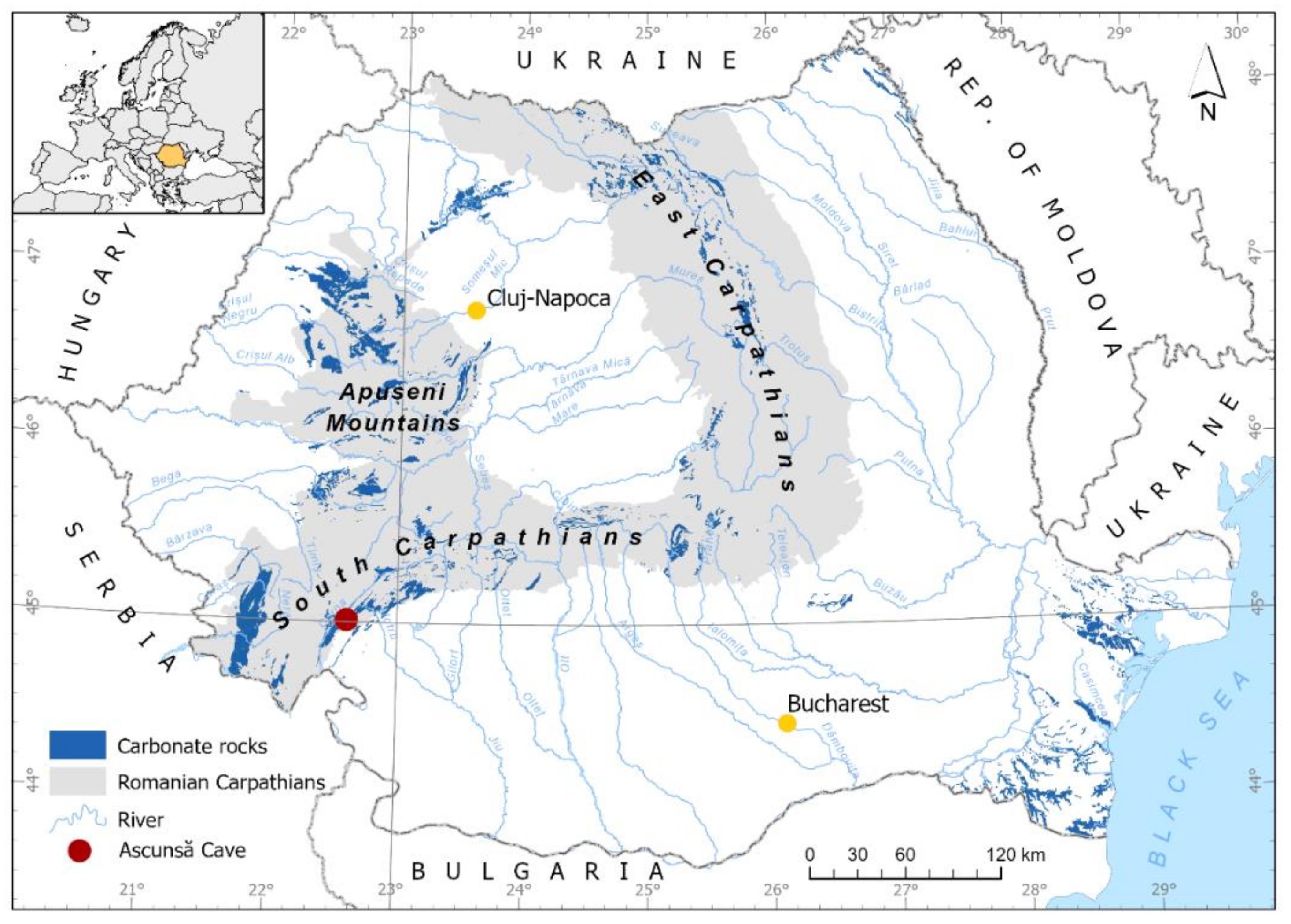
2. Study Site
3. Materials and Methods
3.1. Mineralogical Analysis
3.2. Grain Size
3.3. Magnetic Susceptibility
3.4. Chemical Composition
3.5. Radiocarbon Dating
3.6. δ13C in Soil Organic Matter
3.7. Optically Stimulated Luminescence (OSL) Dating
4. Results
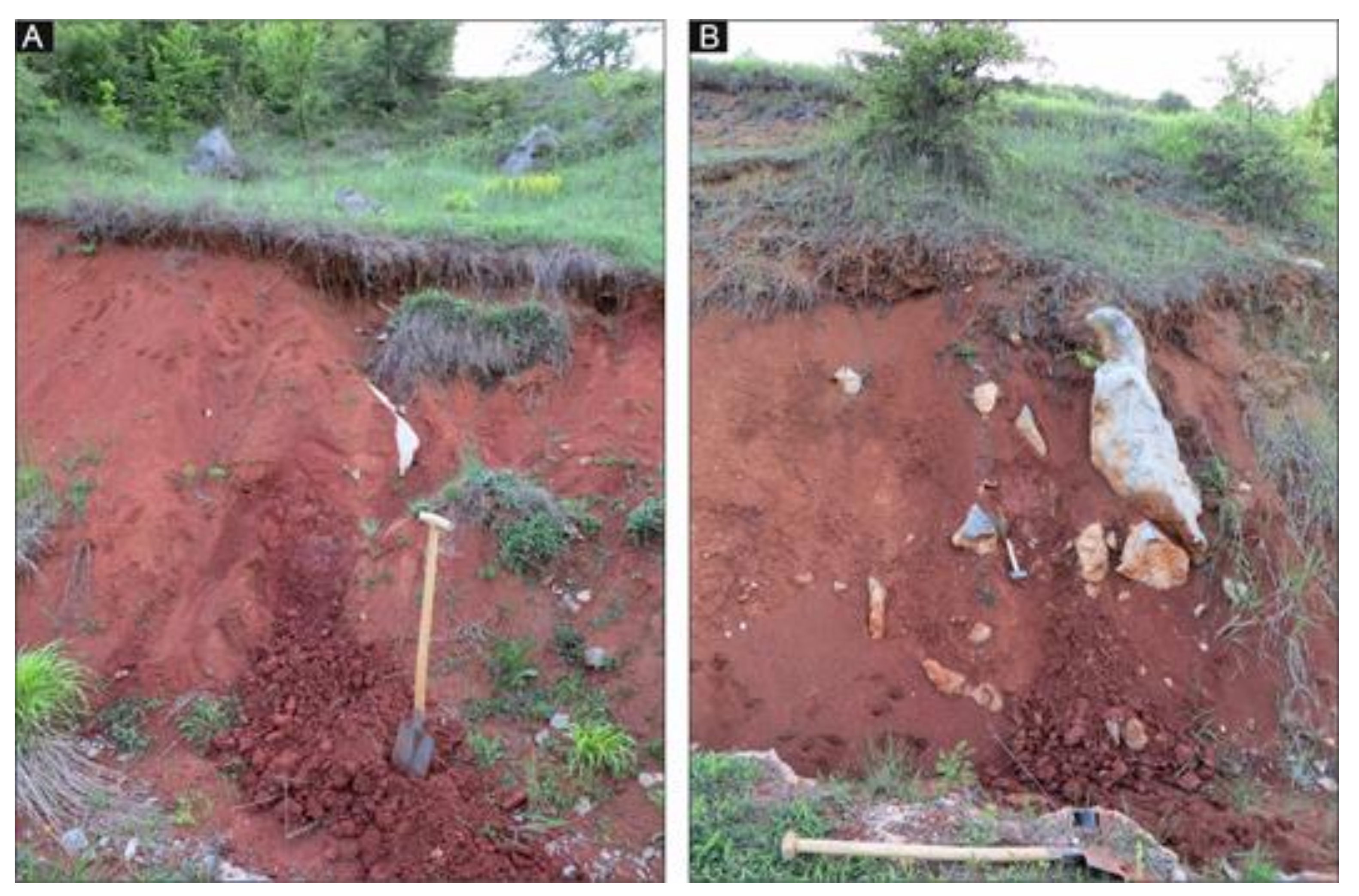
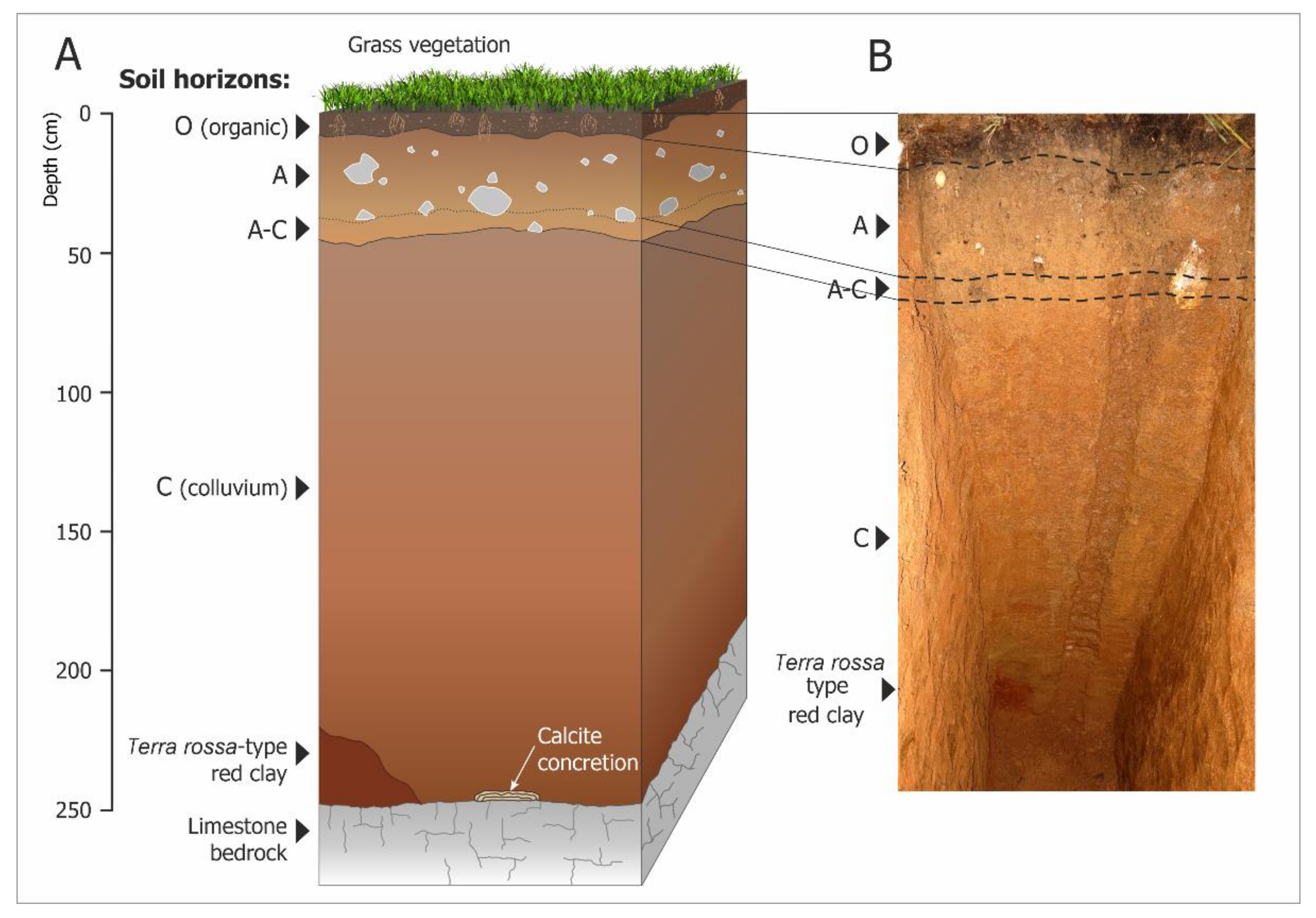
4.1. POM-2 Sedimentary Sequence Description
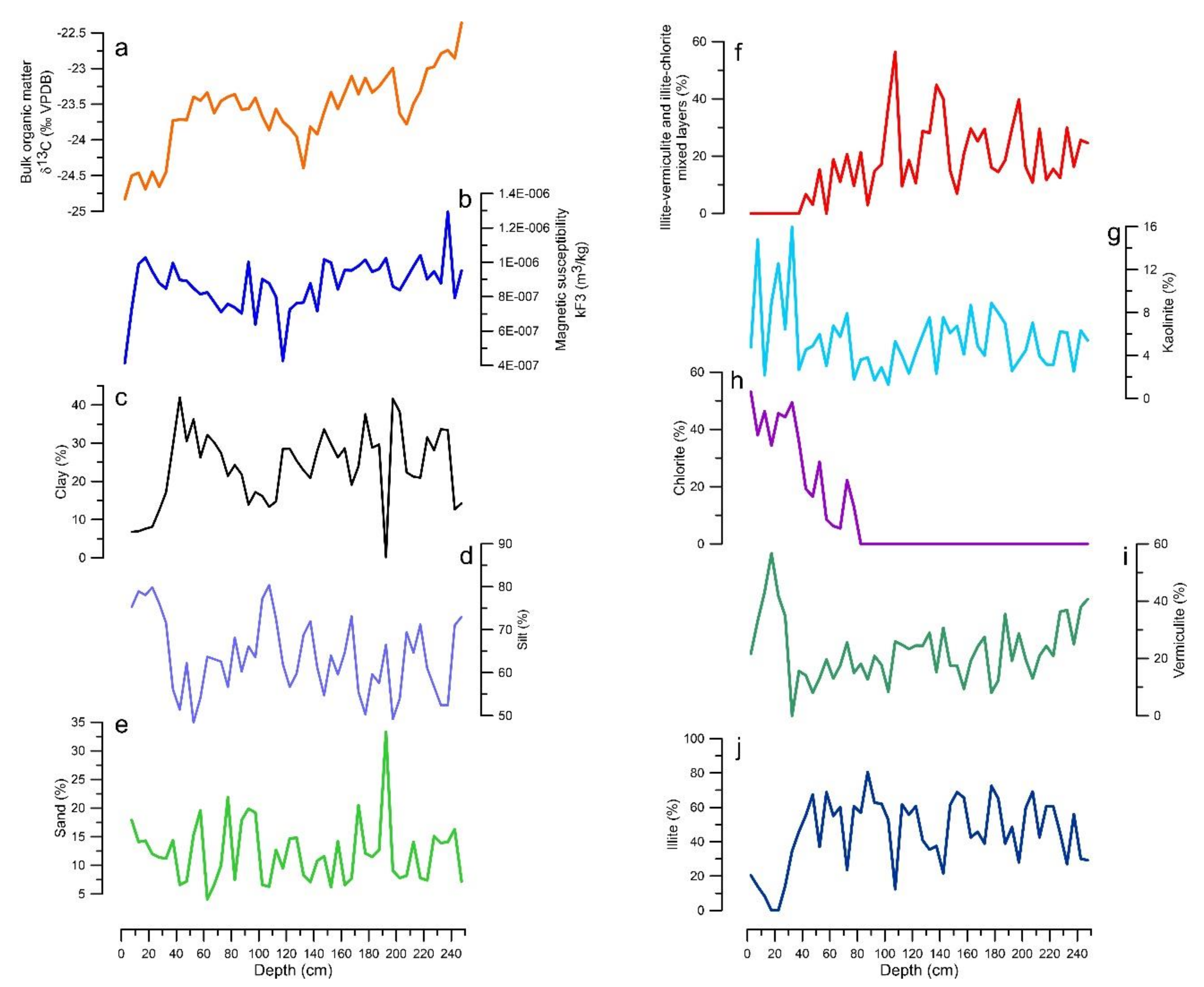
4.2. Grain Size
4.3. Magnetic Susceptibility
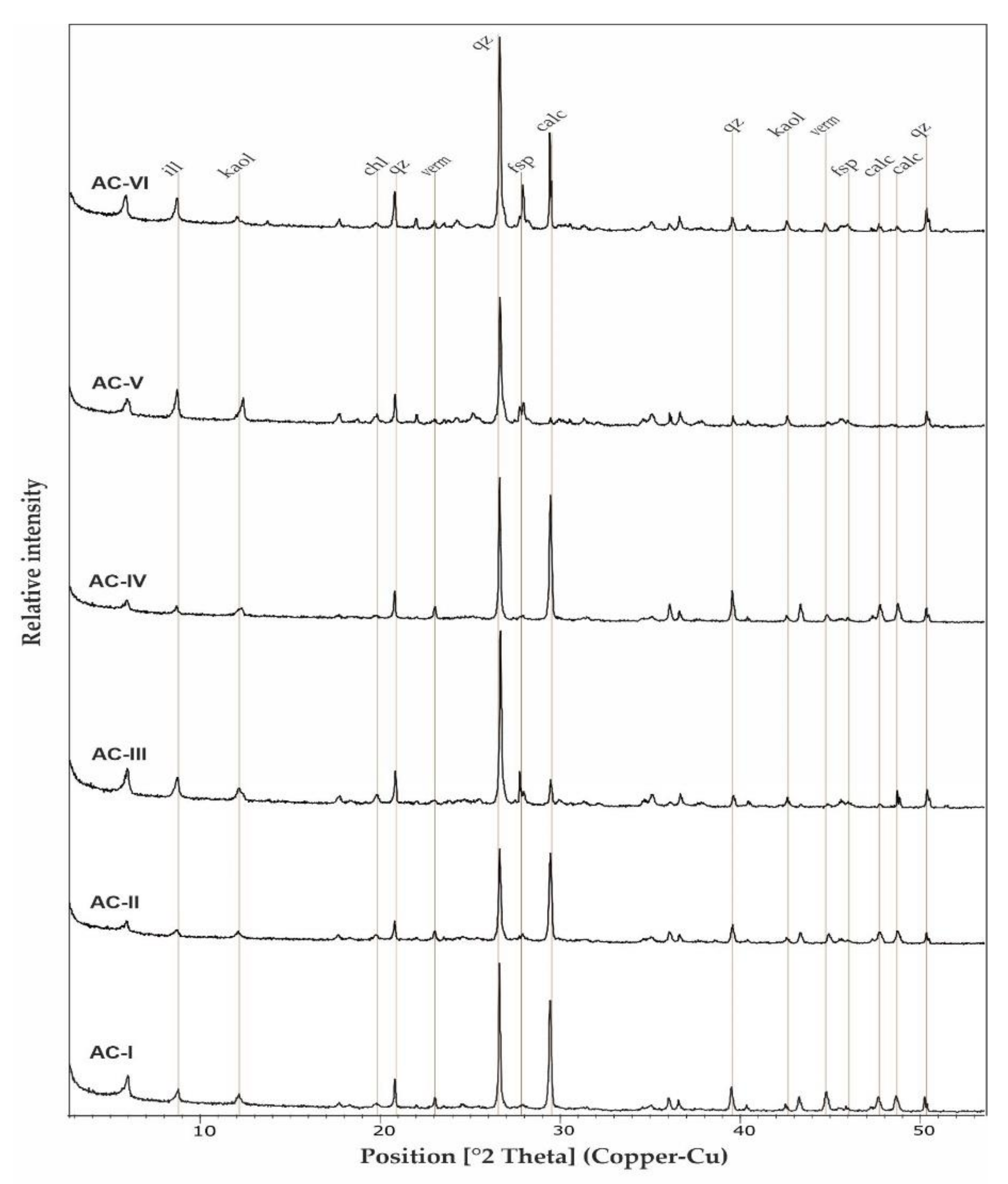
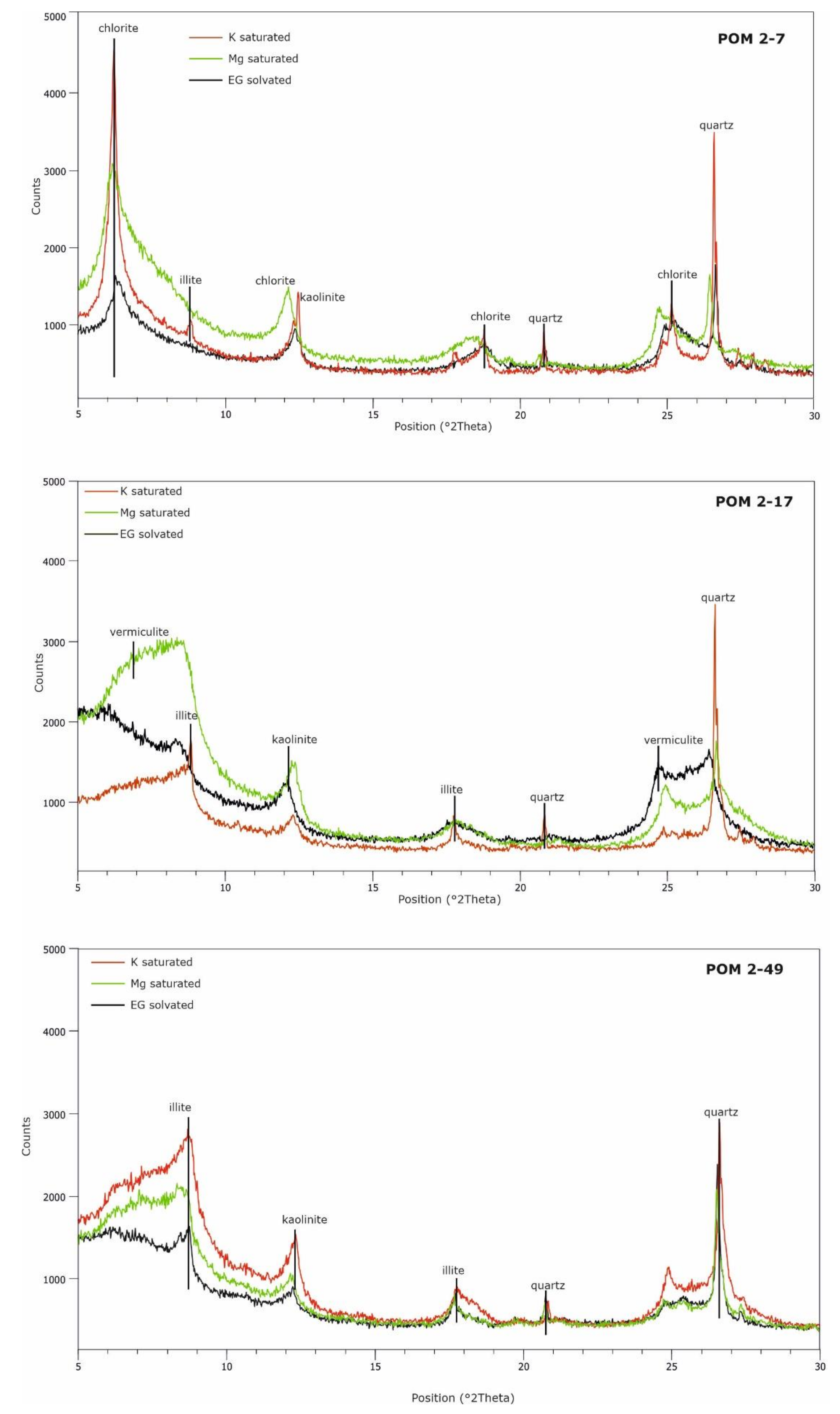
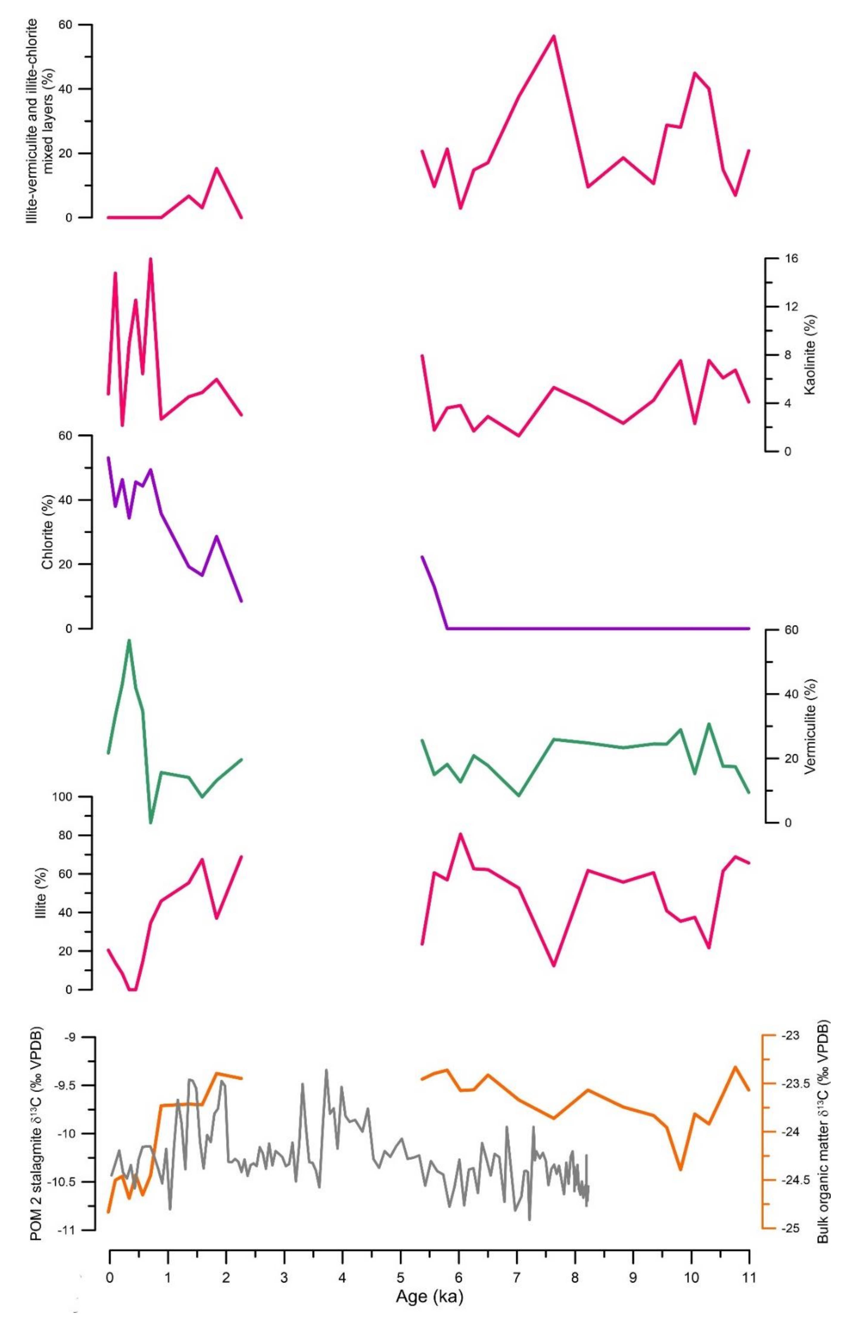
4.4. Mineralogy
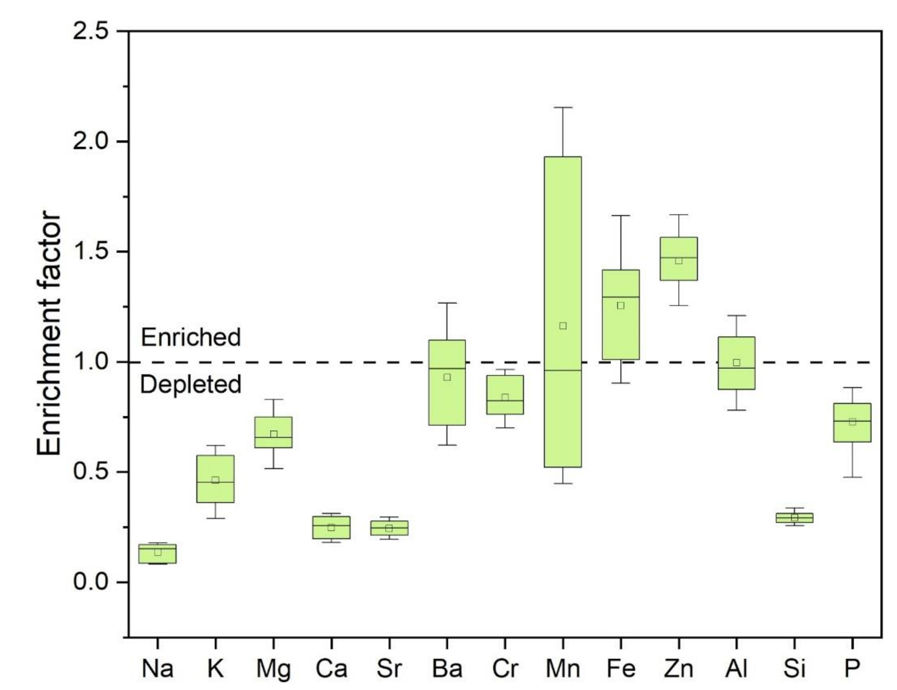
4.5. Chemical Composition
4.6. Carbon Stable Isotopes
4.7. Age-Depth Model
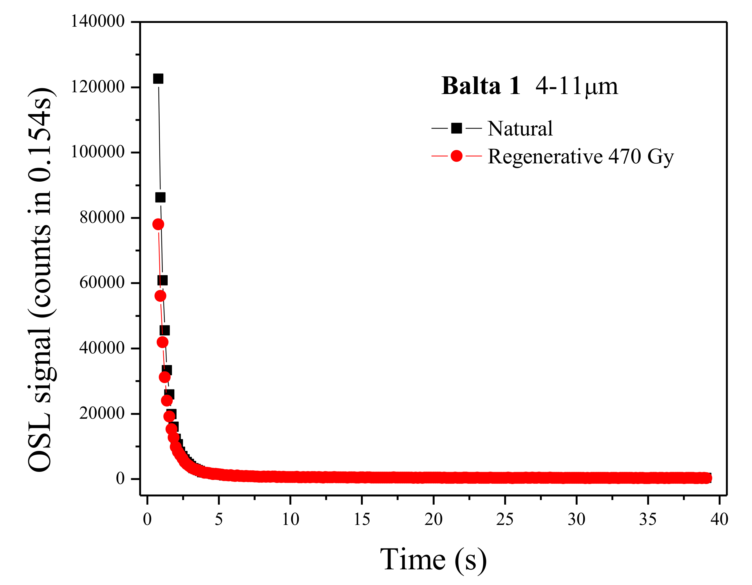
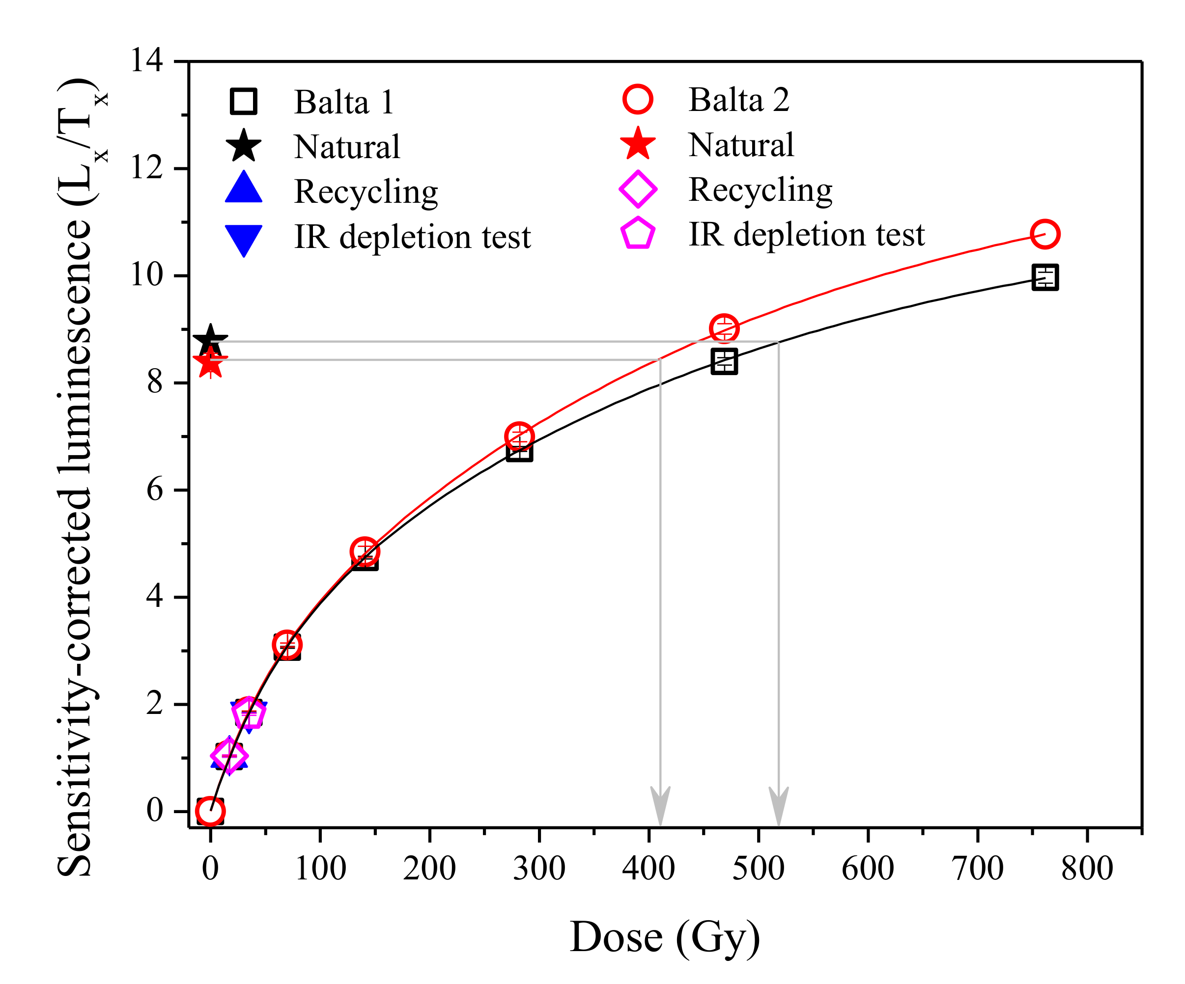
4.8. OSL Dating
5. Discussion
5.1. Depositional Environment
5.2. Age and Environmental Significance of the POM 2 Soil Profile
6. Conclusions
Author Contributions
Funding
Institutional Review Board Statement
Informed Consent Statement
Data Availability Statement
Acknowledgments
Conflicts of Interest
Appendix A

| Sample | Depth (cm) | Illite | Vermiculite | I/Chl | Chlorite | I/V | Kaolinite |
|---|---|---|---|---|---|---|---|
| POM 2-1 | 2.5 | 20.48 | 21.69 | - | 53.07 | - | 4.76 |
| POM 2-2 | 7.5 | 13.99 | 33.23 | - | 38.01 | - | 14.78 |
| POM 2-3 | 12.5 | 8.35 | 43.17 | - | 46.31 | - | 2.16 |
| POM 2-4 | 17.5 | 0 | 56.71 | - | 34.37 | - | 8.92 |
| POM 2-5 | 22.5 | 0 | 41.88 | - | 45.58 | - | 12.54 |
| POM 2-6 | 27.5 | 14.41 | 34.84 | - | 44.31 | - | 6.44 |
| POM 2-7 | 32.5 | 34.66 | 0 | - | 49.39 | - | 15.95 |
| POM 2-8 | 37.5 | 45.95 | 15.62 | - | 35.75 | - | 2.67 |
| POM 2-9 | 42.5 | 55.36 | 14.1 | 6.7 | 19.24 | - | 4.53 |
| POM 2-10 | 47.5 | 67.44 | 8.04 | 3.08 | 16.56 | - | 4.88 |
| POM 2-11 | 52.5 | 36.98 | 13.15 | 15.27 | 28.63 | - | 5.97 |
| POM 2-12 | 57.5 | 68.83 | 19.62 | - | 8.53 | - | 3.02 |
| POM 2-13 | 62.5 | 55.07 | 13.04 | 18.87 | 6.26 | - | 6.76 |
| POM 2-14 | 67.5 | 60.15 | 17.55 | 11.09 | 5.46 | - | 5.75 |
| POM 2-15 | 72.5 | 23.65 | 25.57 | 20.64 | 22.23 | - | 7.92 |
| POM 2-16 | 77.5 | 60.6 | 14.97 | 9.66 | 13 | - | 1.77 |
| POM 2-17 | 82.5 | 56.88 | 18.16 | - | - | 21.36 | 3.6 |
| POM 2-18 | 87.5 | 80.56 | 12.69 | - | - | 2.94 | 3.8 |
| POM 2-19 | 92.5 | 62.64 | 20.86 | - | - | 14.81 | 1.69 |
| POM 2-20 | 97.5 | 62.21 | 17.8 | - | - | 17.09 | 2.89 |
| POM 2-21 | 102.5 | 52.67 | 8.41 | - | - | 37.62 | 1.29 |
| POM 2-22 | 107.5 | 12.39 | 25.91 | - | - | 56.4 | 5.3 |
| POM 2-23 | 112.5 | 61.72 | 24.8 | - | - | 9.53 | 3.95 |
| POM 2-24 | 117.5 | 55.73 | 23.32 | - | - | 18.6 | 2.33 |
| POM 2-25 | 122.5 | 60.62 | 24.52 | - | - | 10.61 | 4.24 |
| POM 2-26 | 127.5 | 40.84 | 24.47 | - | - | 28.78 | 5.91 |
| POM 2-27 | 132.5 | 35.44 | 28.94 | - | - | 28.1 | 7.52 |
| POM 2-28 | 137.5 | 37.51 | 15.29 | - | - | 44.89 | 2.31 |
| POM 2-29 | 142.5 | 21.67 | 30.73 | - | - | 40.05 | 7.54 |
| POM 2-30 | 147.5 | 61.44 | 17.57 | - | - | 14.91 | 6.09 |
| POM 2-31 | 152.5 | 68.85 | 17.46 | - | - | 6.95 | 6.74 |
| POM 2-32 | 157.5 | 65.64 | 9.45 | - | - | 20.81 | 4.1 |
| POM 2-33 | 162.5 | 42.53 | 19.2 | - | - | 29.59 | 8.68 |
| POM 2-34 | 167.5 | 45.75 | 24.14 | - | - | 25.21 | 4.89 |
| POM 2-35 | 172.5 | 38.97 | 27.53 | - | - | 29.5 | 4 |
| POM 2-36 | 177.5 | 72.49 | 8.07 | - | - | 16.03 | 8.87 |
| POM 2-37 | 182.5 | 65.16 | 12.34 | - | - | 14.52 | 7.97 |
| POM 2-38 | 187.5 | 38.96 | 35.49 | - | - | 18.58 | 6.97 |
| POM 2-39 | 192.5 | 48.5 | 19.21 | - | - | 29.72 | 2.57 |
| POM 2-40 | 197.5 | 27.98 | 28.68 | - | - | 39.82 | 3.52 |
| POM 2-41 | 202.5 | 59.77 | 19.62 | - | - | 16.13 | 4.48 |
| POM 2-42 | 207.5 | 69.18 | 13.01 | - | - | 10.78 | 7.03 |
| POM 2-43 | 212.5 | 42.56 | 20.95 | - | - | 29.54 | 3.95 |
| POM 2-44 | 217.5 | 60.7 | 24.4 | - | - | 11.72 | 3.17 |
| POM 2-45 | 222.5 | 60.48 | 20.9 | - | - | 15.5 | 3.13 |
| POM 2-46 | 227.5 | 45.06 | 36.32 | - | - | 12.42 | 6.2 |
| POM 2-47 | 232.5 | 27 | 36.93 | - | - | 29.92 | 6.14 |
| POM 2-48 | 237.5 | 56.05 | 25.07 | - | - | 16.37 | 2.51 |
| POM 2-49 | 242.5 | 30.1 | 37.97 | - | - | 25.61 | 6.32 |
| POM 2-50 | 247.5 | 29.27 | 40.71 | - | - | 24.61 | 5.41 |
Appendix B

| SAMPLE | Grain Size | No. of Aliq (Accepted/Total) | Equivalent Dose (Gy) | Recycling Ratio | IR Depleation Ratio | Recuperation (%) |
|---|---|---|---|---|---|---|
| Balta 1 | 4–11 µm | 12/12 | 514 ± 10 | 1.00 ± 0.01 | 1.00 ± 0.01 | 0.03 ± 0.005 |
| Balta 2 | 4–11 µm | 12/16 | 413 ± 16 | 0.99 ± 0.02 | 0.98 ± 0.01 | 0.02 ± 0.05 |
| Sample | Recovered Dose/Given Dose n = 3 |
|---|---|
| Balta 1 | 0.93 ± 0.01 |
| Balta 2 | 1.05 ± 0.11 |
| Sample | Ra-226 (Bq/kg) | Th-232 (Bq/kg) | K-40 (Bq/kg) |
|---|---|---|---|
| Balta 1 | 36.5 ± 1.0 | 65.1 ± 1.9 | 471 ± 9 |
| Balta 2 | 16.3 ± 0.9 | 60.3 ± 2.2 | 536 ± 7.9 |
| Sample (4–11 µm) | Equivalent Dose (Gy) | Anual Dose (Gy/Ka) | Water Content (%) | Age (Ka) Total Error | Random Error (%) | Systematic Error (%) |
|---|---|---|---|---|---|---|
| Balta 1 | 514 ± 10 | 3.85 ± 0.16 | 9.1 ± 0.9 | 127.9 ± 13.5 | 4.4 | 9.6 |
| Balta 2 | 413 ± 16 | 2.71 ± 0.13 | 33 ± 3.3 | 143.5 ± 18.2 | 6.0 | 11.1 |
References
- Feurdean, A.; Spessa, A.; Magyari, E.K.; Willis, K.J.; Veres, D.; Hickler, T. Trends in biomass burning in the Carpathian region over the last 15,000 years. Quat. Sci. Rev. 2012, 45, 111–125. [Google Scholar] [CrossRef]
- Magyari, E.; Demény, A.; Buczkó, K.; Kern, Z.; Vennemann, T.; Fórizs, I.; Vincze, I.; Braun, M.; Kovacs, I.; Udvardi, B.; et al. A 13,600-year diatom oxygen isotope record from the South Carpathians (Romania): Reflection of winter conditions and possible links with North Atlantic circulation changes. Quat. Int. 2013, 293, 136–149. [Google Scholar] [CrossRef]
- Haliuc, A.; Veres, D.; Brauer, A.; Huba, K.; Hutchinson, S.M.; Begy, R.; Braun, M. Palaeohydrological changes during the mid and late Holocene in the Carpathian area, Central-Eastern Europe. Glob. Planet. Chang. 2017, 152, 99–114. [Google Scholar] [CrossRef] [Green Version]
- Onac, B.P.; Constantin, S.; Lundberg, J.; Lauritzen, S.-E. Isotopic climate record in a Holocene stalagmite from Ursilor Cave (Romania). J. Quat. Sci. 2002, 17, 319–327. [Google Scholar] [CrossRef]
- Constantin, S.; Bojar, A.-V.; Lauritzen, S.-E.; Lundberg, J. Holocene and late Pleistocene climate in the Sub-Mediterranean continental environment: A speleothem record from Poleva Cave (Southern Carpathians, Romania). Palaeogeogr. Palaeoclimatol. Palaeoecol. 2007, 243, 322–338. [Google Scholar] [CrossRef]
- Drăguşin, V.; Staubwasser, M.; Hoffmann, D.L.; Ersek, V.; Onac, B.P.; Veres, D. Constraining Holocene hydrological changes in the Carpathian–Balkan region using speleothem δ18O and pollen-based temperature reconstructions. Clim. Past 2014, 10, 1363–1380. [Google Scholar] [CrossRef] [Green Version]
- Perșoiu, A.; Onac, B.P.; Wynn, J.G.; Blaauw, M.; Ionita, M.; Hansson, M. Holocene winter climate variability in Central and Eastern Europe. Sci. Rep. 2017, 7, 1196. [Google Scholar] [CrossRef] [PubMed] [Green Version]
- Bădăluţă, C.-A.; Perșoiu, A.; Ionita, M.; Piotrowska, N. Stable isotopes in cave ice suggest summer temperatures in East-Central Europe are linked to Atlantic multidecadal oscillation variability. Clim. Past 2020, 16, 2445–2458. [Google Scholar] [CrossRef]
- Onac, B.P.; Forray, F.L.; Wynn, J.G.; Giurgiu, A.M. Guano-derived Δ13C-based paleo-hydroclimate record from Gaura Cu Musca Cave, SW Romania. Environ. Earth Sci. 2014, 71, 4061–4069. [Google Scholar] [CrossRef]
- Cleary, D.M.; Wynn, J.G.; Ionita, M.; Forray, F.L.; Onac, B.P. Evidence of long-term NAO influence on East-Central Europe winter precipitation from a guano-derived Δ15N record. Sci. Rep. 2017, 7, 14095. [Google Scholar] [CrossRef] [Green Version]
- White, W. Cave sediments and paleoclimate. J. Cave Karst Stud. 2007, 69, 76–93. [Google Scholar]
- Lauritzen, S. Reconstructing Holocene climate records from speleothems. In Global Change in the Holocene, 1st ed.; Birks, J., Battarbee, R., Mackay, A., Oldfield, F., Eds.; Hodder Arnold: London, UK, 2003; pp. 242–263. [Google Scholar]
- Wesley, L.D. Fundamentals of Soil Mechanics for Sedimentary and Residual Soils; John Wiley & Sons: Hoboken, NJ, USA, 2009; Chapter 1; pp. 1–11. [Google Scholar]
- Fairchild, I.J.; Smith, C.L.; Baker, A.; Fuller, L.; Spötl, C.; Mattey, D.; McDermott, F. Modification and preservation of environmental signals in speleothems. Earth-Sci. Rev. 2006, 75, 105–153. [Google Scholar] [CrossRef] [Green Version]
- Hendy, C.H. The isotopic geochemistry of speleothems—I. The calculation of the effects of different modes of formation on the isotopic composition of speleothems and their applicability as palaeoclimatic indicators. Geochim. Cosmochim. Acta 1971, 35, 801–824. [Google Scholar] [CrossRef]
- Fohlmeister, J.; Voarintsoa, N.R.G.; Lechleitner, F.A.; Boyd, M.; Brandtstätter, S.; Jacobson, M.J.; Oster, J. Main controls on the stable carbon isotope composition of speleothems. Geochim. Cosmochim. Acta 2020, 279, 67–87. [Google Scholar] [CrossRef]
- Gilg, H.A.; Weber, B.; Kasbohm, J.; Frei, R. Isotope geochemistry and origin of Illite-Smectite and Kaolinite from the Seilitz and Kemmlitz Kaolin deposits, Saxony, Germany. Clay Miner. 2003, 38, 95–112. [Google Scholar] [CrossRef]
- Sheldon, N.D.; Tabor, N.J. Quantitative paleoenvironmental and paleoclimatic reconstruction using paleosols. Earth-Sci. Rev. 2009, 95, 1–52. [Google Scholar] [CrossRef]
- Tabor, N.J.; Montañez, I.P. Oxygen and hydrogen isotope compositions of Permian Pedogenic Phyllosilicates: Development of modern surface domain arrays and implications for paleotemperature reconstructions. Palaeogeogr. Palaeoclimatol. Palaeoecol. 2005, 223, 127–146. [Google Scholar] [CrossRef]
- Hyland, E.G.; Sheldon, N.D.; der Voo, R.V.; Badgley, C.; Abrajevitch, A. A new paleoprecipitation proxy based on soil magnetic properties: Implications for expanding paleoclimate reconstructions. GSA Bull. 2015, 127, 975–981. [Google Scholar] [CrossRef]
- Retallack, G.J. Refining a pedogenic-carbonate CO2 paleobarometer to quantify a middle Miocene greenhouse spike. Palaeogeogr. Palaeoclimatol. Palaeoecol. 2009, 281, 57–65. [Google Scholar] [CrossRef]
- Retallack, G.J. Pedogenic carbonate proxies for amount and seasonality of precipitation in paleosols. Geology 2005, 33, 333–336. [Google Scholar] [CrossRef]
- Sparks, D.L. Environmental soil chemistry: An overview. In Environmental Soil Chemistry, 2nd ed.; Sparks, D.L., Ed.; Academic Press: Burlington, VT, USA, 2003; pp. 1–42. ISBN 978-0-12-656446-4. [Google Scholar]
- Varela, A.N.; Raigemborn, M.S.; Richiano, S.; White, T.; Poiré, D.G.; Lizzoli, S. Late cretaceous paleosols as paleoclimate proxies of high-latitude southern hemisphere: Mata Amarilla Formation, Patagonia, Argentina. Sediment. Geol. 2018, 363, 83–95. [Google Scholar] [CrossRef]
- Velde, B.; Meunier, A. The Origin of Clay Minerals in Soils and Weathered Rocks; Chapter 6; Springer: Berlin, Germany, 2008; Volume 418, pp. 283–299. [Google Scholar] [CrossRef]
- Schulze, D.G. An Introduction to Soil Mineralogy. In Soil Mineralogy with Environmental Applications; John Wiley & Sons, Ltd.: Hoboken, NJ, USA, 2002; pp. 1–35. [Google Scholar] [CrossRef]
- Bădescu, B.; Tîrlă, L. The Karst Map of Romania; Pro Marketing: Reșița, Romania, 2020; p. 5. (In Romanian) [Google Scholar]
- Codarcea, A.; Răileanu, G. Harta Geologică 1:200000, Baia de Aramă; Institute of Geology: Bucharest, Romania, 1968. [Google Scholar]
- Năstăseanu, S.; Bercia, I.; Iancu, V.; Hârtopanu, I. The structure of the South Carpathians (Mehedinți—Banat Area). Guide to Excursion B 2. In Proceedings of the Carpatho-Balkan Geological Association, XII Congress; IGR: Bucharest, Romania, 1981; pp. 1–100. [Google Scholar]
- Mercus, D. Asupra prezenței Urgonianului în regiunea Nadanova, Podișul Mehedinților. Comunicările Acad. R.P.R. 1959, 9, 967–972. [Google Scholar]
- Seghedi, A.; Oaie, G. Volcaniclastic turbidites of the Coşuştea Nappe: A record of late cretaceous arc volcanism in the South Carpathians (Romania). Geol. Balc. 2014, 43, 1–3. [Google Scholar]
- Kunze, G.W.; Dixon, J.B. Pretreatment for mineralogical analysis. In Methods of Soil Analysis; John Wiley & Sons: Hoboken, NJ, USA, 1986; pp. 91–100. ISBN 978-0-89118-864-3. [Google Scholar]
- Rabenhorst, M.C.; Wilding, L.P. Rapid method to obtain carbonate-free residues from limestone and petrocalcic materials. Soil Sci. Soc. Am. J. 1984, 48, 216–219. [Google Scholar] [CrossRef]
- Dumon, M.; Van Ranst, E. PyXRD v0.6.7: A free and open-source program to quantify disordered phyllosilicates using multi-specimen X-ray diffraction profile fitting. Geosci. Model Dev. 2016, 9, 41–57. [Google Scholar] [CrossRef] [Green Version]
- Biscaye, P.E. Mineralogy and sedimentation of recent deep-sea clay in the Atlantic Ocean and adjacent seas and oceans. GSA Bull. 1965, 76, 803–832. [Google Scholar] [CrossRef]
- Brindley, G.W.; Brown, G. Crystal structures of clay minerals and their X-ray identification. Monograph 1980, 5, 495. [Google Scholar] [CrossRef] [Green Version]
- Moore, D.M.; Reynolds, R.C. X-ray Diffraction and the Identification and Analysis of Clay Minerals, 2nd ed.; Oxford University Press: New York, NY, USA, 1997; pp. 335–339. [Google Scholar]
- Gjems, O. Studies on clay minerals and clay-mineral formation in soil profiles in Scandinavia–norwegian Forest: Vollebekk, Norway. Medd. Fra Det Nor. Skogforsoksves. 1967, 21, 303–345. [Google Scholar]
- Soare, B. Mineralogia Argilelor de Varsta Miopliocena din Bazinul Focsani. Ph.D. Thesis, Faculty of Geology and Geophysics, University of Bucharest, Bucharest, Romania, 2016. Unpublished. [Google Scholar]
- Blott, S.J.; Pye, K. GRADISTAT: A grain size distribution and statistics package for the analysis of unconsolidated sediments. Earth Surf. Process. Landf. 2001, 26, 1237–1248. [Google Scholar] [CrossRef]
- Folk, R.L.; Ward, W.C. Brazos river bar: A study in the significance of grain size parameters. J. Sediment. Petrol. 1957, 27, 3–26. [Google Scholar] [CrossRef]
- Hrouda, F. Models of frequency-dependent susceptibility of rocks and soils revisited and broadened. Geophys. J. Int. 2011, 187, 1259–1269. [Google Scholar] [CrossRef] [Green Version]
- Weiss, D.; Shotyk, W.; Appleby, P.G.; Kramers, J.D.; Cheburkin, A. Atmospheric Pb deposition since the industrial revolution recorded by five Swiss peat profiles; enrichment factors, fluxes, isotopic composition and sources K. Environ. Sci. Technol. 1999, 33, 1340–1352. [Google Scholar] [CrossRef]
- Salminen, R.; Batista, M.J.; Bidovec, M.; Demetriades, A.; De Vivo, B.; De Vos, W.; Duris, M.; Gilucis, A.; Gregorauskiene, V.; Halamić, J.; et al. Geochemical Atlas of Europe. Part 1: Background Information, Methodology and Maps; Geological Survey of Finland: Espoo, Finland, 2005; p. 526. [Google Scholar]
- Rudnick, R.L.; Gao, S. The Composition of the Continental Crust. In Treatise on Geochemistry, The Crust; Holland, H.D., Turekian, K.K., Eds.; Elsevier-Pergamon: Oxford, UK, 2003; Volume 3, pp. 1–64. [Google Scholar]
- Boës, X.; Rydberg, J.; Martinez-Cortizas, A.; Bindler, R.; Renberg, I. Evaluation of conservative lithogenic elements (Ti, Zr, Al, and Rb) to study anthropogenic element enrichments in lake sediments. J. Paleolimnol. 2011, 46, 75–87. [Google Scholar] [CrossRef]
- Dumoulin, J.-P.; Comby-Zerbino, C.; Delqué-Količ, E.; Moreau, C.; Caffy, I.; Hain, S.; Perron, M.; Thellier, B.; Setti, V.; Berthier, B.; et al. Status report on sample preparation protocols developed at the LMC14 laboratory, Saclay, France: From sample collection to 14C AMS measurement. Radiocarbon 2017, 59, 713–726. [Google Scholar] [CrossRef]
- Sava, T.B.; Simion, C.A.; Gâza, O.; Stanciu, I.M.; Păceșilă, D.G.; Sava, G.O.; Wacker, L.; Ștefan, B.; Moșu, V.D.; Ghiță, D.G.; et al. Status report on the sample preparation laboratory for radiocarbon dating at the new Bucharest roams center. Radiocarbon 2019, 61, 649–658. [Google Scholar] [CrossRef]
- Stuiver, M.; Polach, H. Discussion: Reporting of 14C data. Radiocarbon 1977, 19, 355–363. [Google Scholar] [CrossRef] [Green Version]
- Blaauw, M.; Christen, J.A. Flexible paleoclimate age-depth models using an autoregressive gamma process. Bayesian Anal. 2011, 6, 457–474. [Google Scholar] [CrossRef]
- Kabacoff, R.I. R in Action. Data Analysis and Graphics with R; Manning Publications: Shelter Island, NY, USA, 2015; p. 579. [Google Scholar]
- R Core Team. R: A Language and Environment for Statistical Computing; R Foundation for Statistical Computing: Vienna, Austria, 2020; Available online: https://www.R-project.org/ (accessed on 1 May 2021).
- Reimer, P.J.; Austin, W.E.N.; Bard, E.; Bayliss, A.; Blackwell, P.G.; Bronk Ramsey, C.; Butzin, M.; Cheng, H.; Edwards, R.L.; Friedrich, M.; et al. The IntCal20 northern hemisphere radiocarbon age calibration curve (0–55 Cal KBP). Radiocarbon 2020, 62, 725–757. [Google Scholar] [CrossRef]
- Wurster, C.M.; McFarlane, D.A.; Bird, M.I. Spatial and temporal expression of vegetation and atmospheric variability from stable carbon and nitrogen isotope analysis of bat guano in the Southern United States. Geochim. Cosmochim. Acta 2007, 71, 3302–3310. [Google Scholar] [CrossRef] [Green Version]
- Forray, F.L.; Onac, B.P.; Tanţău, I.; Wynn, J.G.; Tămaş, T.; Coroiu, I.; Giurgiu, A.M. A Late holocene environmental history of a bat guano deposit from Romania: An isotopic, pollen and microcharcoal study. Quat. Sci. Rev. 2015, 127, 141–154. [Google Scholar] [CrossRef]
- Berden, G.; Engeln, R. Cavity Ring-Down Spectroscopy: Techniques and Applications; John and Wiley and Sons: Hoboken, NJ, USA, 2009; p. 344. [Google Scholar]
- Popovat, M.; Oancea, C.; Edelstein-Heller, D. Terra rossa—Un sol relict in Sud-Vestul Romaniei. Stud. Teh. Economice. Ser. C Pedol. 1970, 17, 7–19. [Google Scholar]
- Avram, A.; Constantin, D.; Veres, D.; Kelemen, S.; Obreht, I.; Hambach, U.; Marković, S.B.; Timar-Gabor, A. Testing polymineral post-IR IRSL and quartz SAR-OSL protocols on Middle to Late Pleistocene loess at Batajnica, Serbia. Boreas 2020, 49, 615–633. [Google Scholar] [CrossRef] [PubMed]
- Murray, A.S.; Wintle, A.G. The single aliquot regenerative dose protocol: Potential for improvements in reliability. Radiat. Meas. 2003, 37, 377–381. [Google Scholar] [CrossRef]
- FAO and IUSS World Reference Base for Soil Resources 2014. International Soil Classification System for Naming Soils and Creating Legends for Soil Maps—Update 2015; World Soil Resources Reports; FAO: Rome, Italy, 2015; ISBN 978-92-5-108369-7. [Google Scholar]
- Patterson, G.T.; Wall, G.J. Within-Pedon variability in soil properties. Can. J. Soil Sci. 1982, 62, 631–639. [Google Scholar] [CrossRef]
- Maher, B.A.; MengYu, H.; Roberts, H.M.; Wintle, A.G. Holocene loess accumulation and soil development at the Western Edge of the Chinese Loess Plateau: Implications for magnetic proxies of palaeorainfall. Quat. Sci. Rev. 2003, 22, 445–451. [Google Scholar] [CrossRef]
- Panaiotu, C.; Constantin, S.; Petrea, C.; Horoi, V.; Panaiotu, C.E. Rock magnetic data of late pleistocene sediments from the Pestera cu Oase and their paleoclimatic significance. In Life and Death at the Pestera cu Oase. A Setting for Modern Human Emergence in Europe; Trinkaus, E., Constantin, S., Zilhão, J., Eds.; Oxford University Press: Oxford, UK, 2012; p. 438. ISBN 978-0-19-539822-9. [Google Scholar]
- Thompson, M.L.; Ukrainczyk, L. Micas. In Soil Mineralogy with Environmental Applications; John Wiley & Sons: Hoboken, NJ, USA, 2002; pp. 431–466. [Google Scholar] [CrossRef]
- Wilson, M.J. The origin and formation of clay minerals in soils: Past, present and future perspectives. Clay Miner. 1999, 34, 7–25. [Google Scholar] [CrossRef]
- Velde, B.; Meunier, A. The Origin of Clay Minerals in Soils and Weathered Rocks; Chapter 8; Springer: Berlin, Germany, 2008; Volume 418, pp. 322–351. [Google Scholar] [CrossRef]
- Barnhisel, R.I.; Bertsch, P.M. Chlorites and hydroxy-interlayered vermiculite and smectite. In Minerals in Soil Environments; John Wiley & Sons: Hoboken, NJ, USA, 1989; pp. 729–788. ISBN 978-0-89118-860-5. [Google Scholar]
- Egli, M.; Merkli, C.; Sartori, G.; Mirabella, A.; Plötze, M. Weathering, mineralogical evolution and soil organic matter along a Holocene soil toposequence developed on carbonate-rich materials. Geomorphology 2008, 97, 675–696. [Google Scholar] [CrossRef]
- Cristea, G.; Cuna, S.M.; Fărcaș, S.; Tanțău, I.; Dordai, E.; Măgdaș, D.A. Carbon stable isotope composition as indicator for climatic changes during the middle and late Holocene in a peat bog from Maramureș Mountains (Romania). Holocene 2014, 24, 15–23. [Google Scholar] [CrossRef]
- Adamiec, G.; Aitken, M. Dose rate conversion factors: Update. Anc. TL 1998, 16, 37–50. [Google Scholar]
- Murray, A.S.; Wintle, A.G. Luminescence dating of quartz using an improved single-aliquot regenerative-dose protocol. Radiat. Meas. 2000, 32, 57–73. [Google Scholar] [CrossRef]
- Wintle, A.G.; Murray, A.S. A review of quartz optically stimulated luminescence characteristics and their relevance in single-aliquot regeneration dating protocols. Radiat. Meas. 2006, 41, 369–391. [Google Scholar] [CrossRef]
- Duller, G.A.T. Distinguishing quartz and feldspar in single grain luminescence measurements. Radiat. Meas. 2003, 37, 161–165. [Google Scholar] [CrossRef]


| Depth | Sample | Na | K | Mg | Ca | Sr | Ba | Cr | Mn | Fe | Zn | Al | Si | P |
|---|---|---|---|---|---|---|---|---|---|---|---|---|---|---|
| 2.5 | POM 2-1 | 2002.9 | 7839.8 | 6256.9 | 7495.4 | 42.4 | 358.3 | 80.7 | 328.5 | 35,077.5 | 102.5 | 63,525.7 | 100,305.3 | 461.7 |
| 17.5 | POM 2-4 | 2014.1 | 6553.4 | 5600.9 | 7825.3 | 45.3 | 327.1 | 77.6 | 328.3 | 32,723.0 | 98.0 | 59,223.3 | 100,798.7 | 458.0 |
| 22.5 | POM 2-5 | 2237.2 | 8242.9 | 6897.4 | 8107.8 | 49.0 | 383.6 | 89.9 | 412.6 | 38,570.1 | 119.4 | 70,232.6 | 112,078.7 | 453.0 |
| 27.5 | POM 2-6 | 2122.0 | 8368.7 | 6907.2 | 8290.4 | 48.0 | 389.6 | 88.2 | 398.3 | 37,513.9 | 106.4 | 69,070.7 | 111,087.7 | 321.0 |
| 32.5 | POM 2-7 | 1878.2 | 7838.4 | 6613.9 | 7965.6 | 39.8 | 382.2 | 79.5 | 516.0 | 36,241.2 | 101.9 | 64,258.9 | 93,893.8 | 391.3 |
| 37.5 | POM 2-8 | 2118.2 | 8881.2 | 7475.9 | 9416.3 | 49.1 | 417.2 | 97.3 | 597.5 | 42,441.1 | 112.8 | 76,239.4 | 112,668.6 | 421.9 |
| 42.5 | POM 2-9 | 1539.4 | 8818.9 | 7280.2 | 10,780.0 | 46.4 | 449.3 | 91.8 | 604.2 | 46,079.6 | 105.0 | 77,266.4 | 107,724.6 | 450.7 |
| 47.5 | POM 2-10 | 1629.8 | 8685.0 | 7070.3 | 10,459.8 | 44.1 | 440.9 | 87.2 | 571.3 | 44,538.3 | 104.3 | 73,220.7 | 105,273.6 | 410.5 |
| 52.5 | POM 2-11 | 1488.8 | 9816.3 | 7354.6 | 10,361.0 | 43.9 | 480.1 | 89.8 | 642.8 | 48,083.4 | 102.0 | 77,584.3 | 111,375.7 | 453.9 |
| 77.5 | POM 2-16 | 1448.5 | 12,878.8 | 8292.2 | 11,653.1 | 47.5 | 612.2 | 98.1 | 1026.0 | 55,400.1 | 113.5 | 83,681.1 | 120,989.0 | 469.1 |
| 102.5 | POM 2-21 | 1086.2 | 13,375.7 | 7843.3 | 11,616.6 | 44.3 | 621.3 | 98.7 | 1664.9 | 53,147.6 | 119.8 | 81,748.4 | 130,369.5 | 431.8 |
| 142.5 | POM 2-29 | 1210.4 | 14,727.3 | 8589.1 | 11,515.0 | 39.6 | 669.3 | 93.5 | 1637.4 | 51,878.0 | 115.2 | 79,971.6 | 125,907.8 | 569.9 |
| 182.5 | POM 2-37 | 1159.7 | 15,710.0 | 8430.0 | 12,916.1 | 42.8 | 688.5 | 108.8 | 1687.3 | 56,800.7 | 138.2 | 88,959.3 | 138,943.7 | 563.1 |
| 222.5 | POM 2-45 | 1148.6 | 14,142.9 | 7859.3 | 12,865.7 | 46.4 | 603.7 | 107.7 | 1106.3 | 56,355.5 | 146.1 | 92,621.4 | 137,597.3 | 678.3 |
| 247.5 | POM 2-50 | 1184.2 | 15,414.1 | 8338.8 | 10,437.5 | 43.6 | 628.5 | 123.2 | 1869.5 | 55,051.9 | 154.3 | 87,108.6 | 128,971.9 | 655.4 |
| Sample | Laboratory | Depth (cm) | 14C Age Yrs BP ± Error or Remarks | 14C Activity (F14C ± Error) | Calibrated Years (BP or AD) | Date Used (BP) |
|---|---|---|---|---|---|---|
| Bulk organic matter | ||||||
| POM 2-7 | LMC14 | 32.5 | 715 ± 30 | - | 717–564 | 641 |
| POM 2-8 | LMC14 | 37.5 | 635 ± 30 | - | 661–553 | 607 |
| POM 2-9 | ROAMS | 42.5 | 1457 ± 52 | - | 1509–1284 | 1397 |
| POM 2-11 | ROAMS | 52.5 | 1847 ± 45 | - | 1872–1621 | 1747 |
| POM 2-13 | ROAMS | 62.5 | 2538 ± 35 | - | 2749–2494 | 2622 |
| POM 2-15 | LMC14 | 72.5 | 4680 ± 30 | - | 5476–5319 | 5398 |
| POM 2-20 | LMC14 | 97.5 | 5660 ± 35 | - | 6531–6319 | 6425 |
| POM 2-25 | LMC14 | 122.5 | 8380 ± 35 | - | 9485–9296 | 9391 |
| POM 2-30 | LMC14 | 147.5 | 9325 ± 40 | - | 10,662–10,384 | 10,523 |
| POM 2-35 | LMC14 | 172.5 | 9835 ± 45 | - | 11,391–11,186 | 11,289 |
| POM 2-40 | LMC14 | 197.5 | 7880 ± 35 | - | 8977–8559 | 8768 |
| POM 2-45 | LMC14 | 222.5 | 7770 ± 35 | - | 8629–8413 | 8530 |
| POM 2-50 | LMC14 | 247.5 | 6710 ± 35 | - | 7665–7508 | 7587 |
| Root fragments | ||||||
| POM 2-9 | ROAMS | 42.5 | modern | 1.2062 ± 0.007 | AD 1983–1987 (97.55%) 2σ | 1985 |
| POM 2-11 | ROAMS | 52.5 | modern | 1.1266 ± 0.008 | AD 1991–1997 (97.55%) 2σ | 1994 |
| POM 2-13 | ROAMS | 62.5 | modern | 1.1752 ± 0.008 | AD 1986–1990 (97.55%) 2σ | 1988 |
| POM 2-44 | ROAMS | 217.5 | modern | 1.0749 ± 0.008 | AD 2001–2007 (97.55%) 2σ | 2004 |
| POM 2-49 | ROAMS | 242.5 | modern | 1.1393 ± 0.008 | AD 1990–1995 (97.55%) 2σ | 1993 |
| SAMPLE (4–11 µm) | Equivalent Dose (Gy) | Annual Dose (Gy/ka) | Water Content (%) | Age (ka) Total Error | Random Error (%) | Systematic Error (%) |
|---|---|---|---|---|---|---|
| Balta 1 | 514 ± 10 | 3.85 ± 0.16 | 9.1 ± 0.9 | 127.9 ± 13.5 | 4.4 | 9.6 |
| Balta 2 | 413 ± 16 | 2.71 ± 0.13 | 33 ± 3.3 | 143.5 ± 18.2 | 6.0 | 11.1 |
Publisher’s Note: MDPI stays neutral with regard to jurisdictional claims in published maps and institutional affiliations. |
© 2021 by the authors. Licensee MDPI, Basel, Switzerland. This article is an open access article distributed under the terms and conditions of the Creative Commons Attribution (CC BY) license (https://creativecommons.org/licenses/by/4.0/).
Share and Cite
Faur, L.; Drăgușin, V.; Dimofte, D.; Forray, F.L.; Ilie, M.; Marin, C.; Mănăilescu, C.; Mirea, I.C.; Panaiotu, C.G.; Soare, B.; et al. Multi-Proxy Study of a Holocene Soil Profile from Romania and Its Relevance for Speleothem Based Paleoenvironmental Reconstructions. Minerals 2021, 11, 873. https://doi.org/10.3390/min11080873
Faur L, Drăgușin V, Dimofte D, Forray FL, Ilie M, Marin C, Mănăilescu C, Mirea IC, Panaiotu CG, Soare B, et al. Multi-Proxy Study of a Holocene Soil Profile from Romania and Its Relevance for Speleothem Based Paleoenvironmental Reconstructions. Minerals. 2021; 11(8):873. https://doi.org/10.3390/min11080873
Chicago/Turabian StyleFaur, Luchiana, Virgil Drăgușin, Daniela Dimofte, Ferenc Lázár Forray, Maria Ilie, Constantin Marin, Cristian Mănăilescu, Ionuț Cornel Mirea, Cristian George Panaiotu, Barbara Soare, and et al. 2021. "Multi-Proxy Study of a Holocene Soil Profile from Romania and Its Relevance for Speleothem Based Paleoenvironmental Reconstructions" Minerals 11, no. 8: 873. https://doi.org/10.3390/min11080873
APA StyleFaur, L., Drăgușin, V., Dimofte, D., Forray, F. L., Ilie, M., Marin, C., Mănăilescu, C., Mirea, I. C., Panaiotu, C. G., Soare, B., Timar-Gabor, A., & Tîrlă, M. L. (2021). Multi-Proxy Study of a Holocene Soil Profile from Romania and Its Relevance for Speleothem Based Paleoenvironmental Reconstructions. Minerals, 11(8), 873. https://doi.org/10.3390/min11080873