Mounted Single Particle Characterization for 3D Mineralogical Analysis—MSPaCMAn

Abstract

This paper demonstrates a new method to classify mineral phases in 3D images of particulate materials obtained by X-ray computed micro-tomography (CT), here named mounted single particle characterization for 3D mineralogical analysis (MSPaCMAn). The method allows minimizing the impact of imaging artefacts that make the classification of voxels inaccurate and thus hinder the use of CT to characterize natural particulate materials. MSPaCMAn consists of (1) sample preparation as particle dispersions; (2) image processing optimized towards the labelling of individual particles in the sample; (3) phase identification performed at the particle level using an interpretation of the grey-values of all voxels in a particle rather than of all voxels in the sample. Additionally, the particle’s geometry and microstructure can be used as classification criteria besides the grey-values. The result is an improved accuracy of phase classification, a higher number of detected phases, a smaller grain size that can be detected, and individual particle statistics can be measured instead of just bulk statistics. Consequently, the method broadens the applicability of 3D imaging techniques for particle analysis at low particle size to voxel size ratio, which is typically limited due to unreliable phase classification and quantification. MSPaCMAn could be the foundation of 3D semi-automated mineralogy similar to the commonly used 2D image-based semi-automated mineralogy methods.

1. Introduction

The demand for mineral resources is expected to increase in order to carry on the green energy transition [1]. For example, cobalt and lithium are necessary for battery components of electric vehicles and rare-earth elements are needed for electric generators of wind turbines. Due to the steady decrease in ore grades, the demand for raw materials must be sustained by more efficient minerals processing and recycling technologies. It is our hypothesis that evolving from the currently used material characterization techniques towards more comprehensive 3D particle-based characterization could be the starting point of more efficient particle processing methods.

2D imaging techniques typically used to characterize raw materials have an associated stereological bias [2,3,4] due to the loss of information (what is under the surface), whereas 3D imaging can provide a full description of a material. The stereological bias increases with the complexity and the texture variability within an ore. That suggests that 2D and bulk particle characterization could neglect properties of individual particles that are important to describe and to simulate a process [5,6,7]. For example, the separation of particles from a feed material into a concentrate or into tailings are typically the sum of discrete particle events that depend mostly on the particle properties and not necessarily on the overall properties of all particles [6,8,9]. Since particles are three-dimensional objects, a complete description of particle size, geometry, morphology, composition and distribution of phases inside the particle or on the particle’s surface requires 3D measurements. Such 3D properties determine whether a particle can be separated using any particle processing technique. For instance, the surface properties of particles are the most relevant to determine their flotation behaviour, but shape, size and density can also contribute to the particle’s behaviour [10]. As another example, magnetic susceptibility is the key property for separating magnetic particles, but it has been demonstrated that the particle size class also affects the separation efficiency [11]. In conclusion, using more realistic particle properties associated to a three-dimensional analysis is expected to improve predictive mineral processing models that can benefit process efficiency [8].

X-ray computed micro-tomography (CT) has risen in the past decade as the prime technique for 3D imaging [12,13]. The 3D microstructure of samples can be segmented into regions with similar grey-values (e.g., mineral or group of minerals) for analyses and quantification [12]. For example, volume, grain sizes, surface area, spatial distribution and associations of individual particles or phases can be quantified [14,15,16,17,18,19,20]. Despite the advantages of measuring 3D microstructures, classifying the phases composing those microstructures based on grey-values remains challenging due to imaging artefacts [21,22] that cause a broadening of the grey-scale interval that can be attributed to a phase [23,24]. Consequently, the ability to distinguish between phases is reduced and less accurate, especially for complex multiphase materials containing small grains characteristic of ore particles [25].

Here, we propose a workflow to classify phases in particulate materials using CT. The workflow will be referred to as Mounted Single Particle Characterization for 3D Mineralogical Analysis (MSPaCMAn). This workflow includes sample preparation in the form of particle dispersions, which reduces the amount of typical CT artefacts in the 3D image and separates the particles. This simplifies the segmentation of individual particles that, subsequently, can be analysed individually. MSPaCMAn is applied to classify minerals or mineral groups present in three different natural particulate materials of different complexities. An improved ability to differentiate phases with similar attenuation contrast is demonstrated and discussed as the potential start of a semi-automated 3D particle characterization technique.

2. Materials and Methods

2.1. Background of the Method

The 3D microstructure of particles measured by CT is represented by voxelized images where the grey-value of a voxel is in theory a function of the electron density of the material within the voxel [13]. However, this correlation of grey-scale vs phase composition is never obtained in practice due to image artefacts arising from physical limitations inherent to X-ray transmission techniques such as CT [26]. For example, beam hardening (BH) is caused by an increase of the overall energy of the X-ray beam as lower energy X-rays are more likely to be attenuated through the sample. This results in artificially higher grey-values of voxels at the edge of a region relative to its centre. Consequently, BH broadens the range of grey-values that correspond to a phase, thus making the grey-scale also dependent on the location of the voxel within the sample and on the heterogeneity of the sample [24]. Another problem is the partial volume effect (PVE) that is observed at voxels composed of more than one phase, e.g., at interphases. The grey-value of those voxels represents the attenuation coefficient of all phases inside the voxel, proportionally to their volume fraction [23]. Consequently, depending on shape, size and the number of phases in a particle, the PVE may affect a significant portion of the particle’s volume and adds to the uncertainty of phase classification based only on grey-scale. Additionally, the size and shape of the source (not a point) and the conical shape of the X-ray beam cause cone beam artefacts (CBA). Depending on the scanning conditions and type of CT scanner, a point in the sample is typically detected at more than one pixel in the detector. Consequently, a pixel in the detector collects information from multiple locations in a sample. In practice, CBA adds to the blurriness of interphases caused by PVE and affects at least three to five voxels at the edge of a grain. Moreover, the probabilistic nature of the physical processes at the source, sample and detector results in some degree of randomness associated to the grey-values. This is typically referred to as image noise.

The sum of all the factors contributing to the grey-value of a voxel, beyond the value expected for a specific mineral, signify that each mineral phase is represented by an interval of grey-values and not by a unique value. Therefore, minimizing imaging artefacts would shorten the interval of grey-values corresponding to a phase, which would improve the ability to classify phases based on grey-values. Additionally, the challenge of phase classification due to image artefacts increases with the complexity and the heterogeneity of the particles. For example, lower grain size to voxel size ratios increase the proportion of voxels affected by artefacts [23]. Consequently, current 3D imaging methods to analyse ore particles with the sizes that are often used for minerals processing are limited by the ability to classify phases. In conclusion, more reliable methods used to classify mineral phases from 3D images of ore particulate materials need to reduce the CT imaging artefacts described above.

MSPaCMAn consists of a workflow that aims to ease phase classification of 3D images of particulate materials by (1) scanning particle dispersions after specific sample preparation as a way to homogenise BH throughout the sample and to reduce PVE and CBA; (2) classifying phases at the particle level, which simplifies the interpretation of grey-values.

2.2. Method Description

The MSPaCMAn workflow is subdivided into three interconnected steps (Figure 1): sample preparation and scanning (a), image processing towards individual particle analysis (b), and classification of particle properties, geometrical (c) and mineralogical (d). The general workflow can be broadly utilized to analyse any particulate material, although the specific parameters used in each step are neither unique nor universal. Therefore, while following the same workflow, the parameters that are appropriate for one particle system may not work for others. Additionally, different parameters can be optimized to specific mineralogical systems and to the type of particle properties that are under study. Next, the different parameters that must be considered in each step of the workflow are discussed and demonstrated to ease the classification of phases present in three particulate materials from different geological origins.

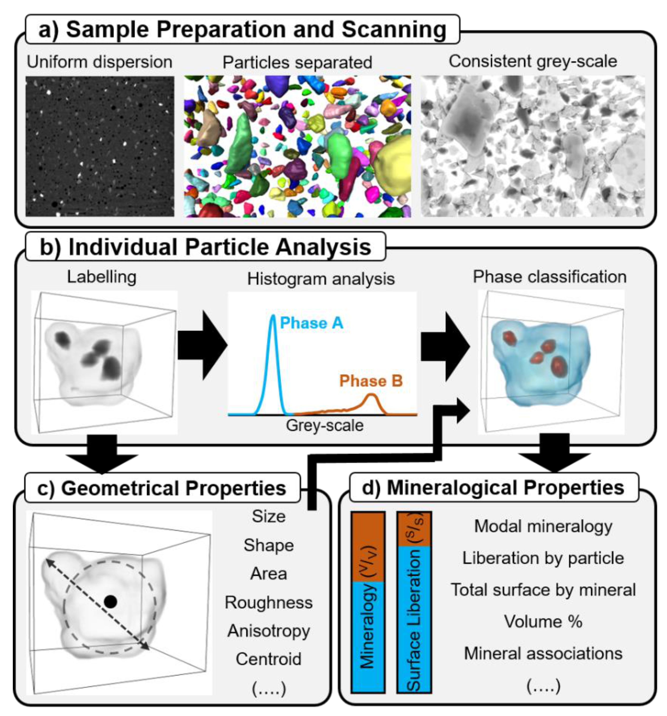
2.2.1. Sample Preparation and Scanning

The ideal sample consists of a uniform particle dispersion in a cylindrical vial where particles are distant from their neighbour particles. The uniform distribution of particles throughout the sample’s volume and the cylindrical shape would make the overall energy of the X-ray beam similar at all sample’s cross-sections. Therefore, beam hardening and noise would be similar throughout the sample. In practice, this allows a direct comparison of voxel grey-values independent of the voxel position within a sample; thus the grey-values are only dependent on the voxel composition. The second requisite of a particle dispersion is that a particle should be separated from all its neighbour particles by a distance of several voxels. Larger distances would ease the segmentation of individual particles in the next step of the workflow and it would reduce the number of voxels affected by PVE, i.e., removes contact points between particles as interphases. The ideal sample described here is difficult to achieve in practice [27]. Deviations from the ideal standard may be corrected on the next steps of the workflow or could otherwise add uncertainty to phase classification [28,29].

Here, a general sample preparation method is demonstrated as a promoter of ideal particle dispersions described in the previous paragraph. The method consists of mixing the particles of the material to be analysed with particles of a spacer material. The mixture of particles is embedded in a hardening resin inside a vial. Several parameters can be optimized relative to the size of the sample’s particles in order to promote a uniform dispersion of particles; for example, the percentage of the sample’s particles in the mixture with the spacer, and the size fraction of the spacer. Spacer size fractions smaller than the sample’s particle size help in creating space between particles. It is also necessary to add larger size fractions of the spacer to prevent settling and gravity segregation of denser particles. It is important that the spacer consists of a material with an attenuation coefficient significantly different from the sample’s components; preferably a material with lower attenuation coefficient such as organic materials.

The scanning conditions and the reconstruction parameters should primarily aim at reducing the imaging artefacts and at providing a voxel size significantly smaller than the particles’ size. For example, samples with very dense materials must be scanned at higher energies, using thicker or denser filters to reduce BH and scattering. Optimizing the contrast between phases should also be kept in mind, although it is less important compared to traditional analysis [30]. This is due to a gain in phase resolution that can be achieved with MSPaCMAn, as it will be demonstrated in this paper. In order to obtain comparable results when analysing multiple samples, the same parameters and conditions should be used. Quantitative studies should also consider how many particles are necessary to create a statistically representative sample [4,31], which is a quantity inversely proportional to the scan resolution and to the sample’s diameter.

2.2.2. Individual Particle Analysis

The image processing aims to be simple in order to allow semi-automation and to reduce the bias associated with traditional phase segmentation methods. With these aims in mind, segmentation is performed at the particle level and not at the grain (phase) level as is done in typical 3D image analysis. First, the individual particles are segmented, which allows breaking down the 3D image into small regions (one particle is one region) that are comparable in terms of grey-scale and can further be analyzed individually [32,33]. Segmentation of individual particles can be achieved using thresholding or artificial intelligence methods [34], as will be exemplified in this paper. The quality of the segmentation may be improved by applying an image filter to reduce noise previous to segmentation, or by using a watershed algorithm to separate particles that are segmented as a single region [35]. The image processing techniques to be applied should be tailored to the quality of the sample preparation and to the peculiarity of the particle system, e.g., composition, particle size and shape.

Once the particles have been segmented, they should be labelled, i.e., each particle has a unique identifier, which allows further analysis of single particles. For each particle, two main types of information can be obtained, geometrical properties (Figure 1c) and mineralogical properties (Figure 1d). The geometric properties can be directly calculated from a binary image of the particle (without grey-scale information). The mineralogical properties consist of the type, amount and distribution of phases inside a particle. Measuring these properties starts with the classification of the phases in the particle, which can be derived from the grey-values of all voxels in the particle. Figure 1 shows that the phase classification can be facilitated by plotting the grey-values of voxels as a function of their frequency in a particle, namely its voxel intensity histogram.

The analysis of a particle’s histogram consists of first identifying the peak positions that can be directly correlated to a phase (further referred to as main peaks) and the peaks that correspond to voxels containing more than one phase (PVE) or are affected by image artefacts (further referred to as minor peaks). The main peaks should be dominant, i.e., be frequencies higher than minor peaks, and should appear around similar grey-values for different particles composed of the same phase. Minor peaks typically have maximum frequencies significantly lower than the main peaks, and their grey-value can vary depending on the particle’s complexity, i.e., shape, size, and the number of phases in the particle. Different information can be drawn from each type of peak. The grey-values corresponding to the main peaks can be used to classify the phases present in the particle. The minor peaks are suitable for identifying specific associations and microstructures containing more than one phase. This also opens the possibility to quantitatively correct the information contained in voxels corresponding to small peaks. For instance, PVE between two phases can be corrected based on the individual particle properties and on the information about the position of the main peaks (known phases in the particle) using a linear interpolation between both peak positions [23]. Nevertheless, this paper will focus on the qualitative classification of the main peaks and on the use of particle-specific criteria, beyond grey-scale criteria, to classify the particle composition.

Depending on the sample’s composition and on the image quality, the histogram analysis may be simplified by promoting regions of similar grey-scale (grains), by removing noise and/or by reducing grey-scale gradients using image filters. In practice, this results in fewer peaks, each with higher frequency. This may simplify the interpretation of the histogram but should be used with caution, so that the position of the peaks is not changing and that real information is not lost. Note that the same histogram analysis can be applied to all voxels in a particle, which relates to the modal mineralogy; to only the surface voxels, which relates to the surface liberation; or only to interphase voxels, which relates to the association between minerals within the particle.

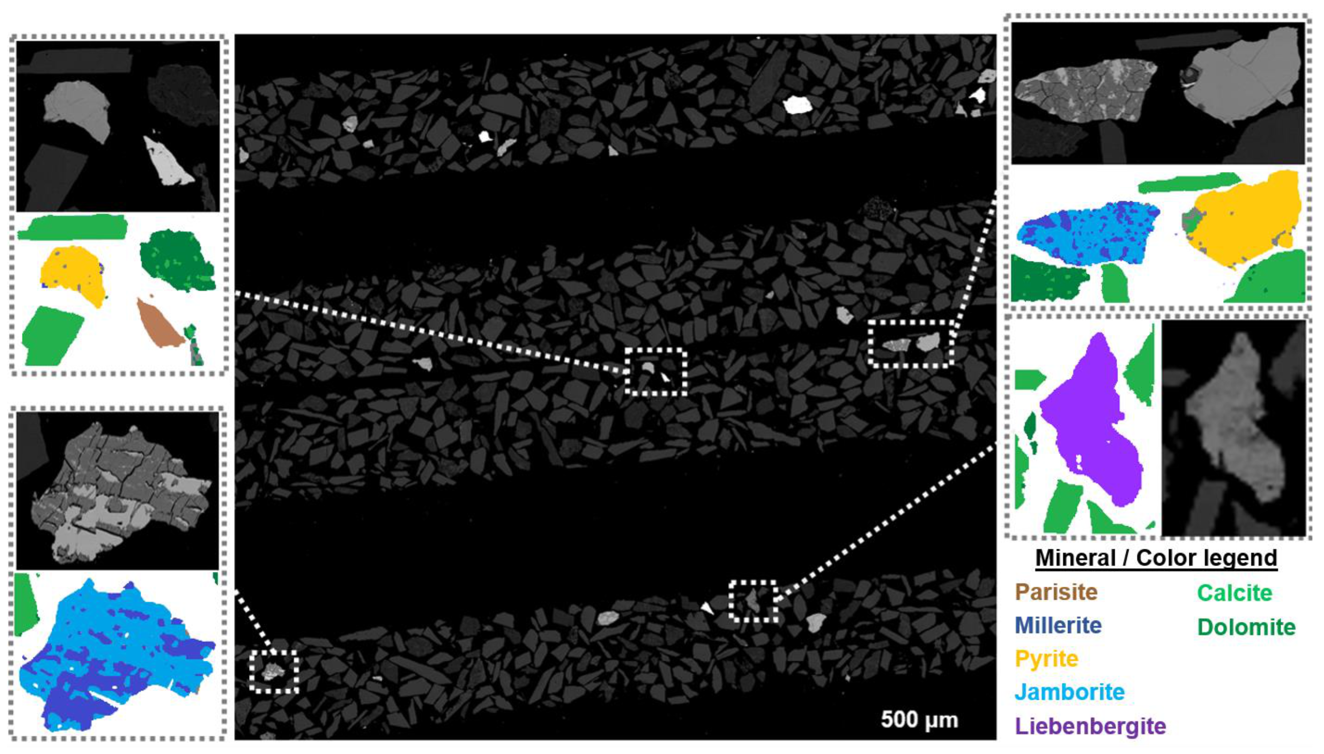
2.3. Mineralogical Validation

Preliminary mineralogical information about the main phases in a sample is advantageous in order to optimize the scanning conditions that maximize the contrast between phases, i.e., increase the distance between main peaks in the histogram. The distance between peaks can be anticipated using, for example, the National Institute of Standards and Technology (NIST) database or software that simulates the attenuation coefficients of minerals based on chemical composition and density [36]. The position of main peaks (or interval of grey-values) can be ranked based on the attenuation of the phases expected in the sample, e.g., higher X-ray attenuation coefficient implies higher grey-values. This validation method will be exemplified for the sample named Qz/Py.

If the sample’s mineralogy is unknown, then correlation of the 3D image with other imaging techniques capable of phase classification such as SEM-based automated mineralogy [37] or optical microscopy is necessary. For example, by comparing a classified image from mineral liberation analysis (MLA) of a cross-section of the sample with the corresponding slice in a CT image, it is possible to determine the range of grey-values that correspond to the phases visible at that cross-section [14,23,26]. This validation method will be exemplified for the samples named Carbonate and Sheelite ore. New CT techniques that allow the measurement of chemical information about the elements inside a sample are currently under development, e.g., spectral CT [26,38] or hyperspectral CT [39]. Such methods have the advantage of not requiring sample preparation nor the complex image processing associated with correlative methods.

2.4. Method Demonstration

Three materials were analysed following the MSPaCMAn workflow with the goal of demonstrating the advantages and the limitations of the workflow as well as the versatility of each step to be adjusted to different particulate materials. Sugar, polymethyl metacrylate (PMMA) and graphite with different size fractions were used as spacer. Sugar has the advantages of being widely available, cheap and easily crushed and sieved into specific size fractions. However, it is soluble in water and organic solvents used for polishing, thus it is not appropriate to be used if the sample is to be correlated to MLA. PMMA and graphite are insoluble in water, thus can be used when the sample is to be cut and polished for MLA analysis. The disadvantage of PMMA is that it is difficult to crush and to sieve into specific size fractions, and the graphite is difficult to obtain pure in larger size fractions. The size fractions of spacer particles were adapted to the particle size of the sample, i.e., size fractions smaller than the sample’s particle sizes help creating space between particles and size fractions about the same size of the sample’s particles help preventing the gravity segregation of denser particles. Different image processing parameters were used depending on the complexity of the material.

All samples where scanned in a CoreTom from XRE–Tescan and reconstructed using the XRE recon software (v1.1.0.14, XRE–Tescan, Ghent, Belgium) that uses a cone beam filtered back projections algorithm. Image processing was performed using Avizo software (v9.3.0, Thermo Fisher Scientific, Waltham, MA, USA), FIJI (v1.53c, https://imagej.nih.gov/ij/) and Dragonfly software (v2021.1, Objects Research Systems, Montreal, Quebec, Canada). Note that all images were processed as 16-bit (grey-scale between 0–65535). Data visualization in the particle histograms was compressed to 650 bins.

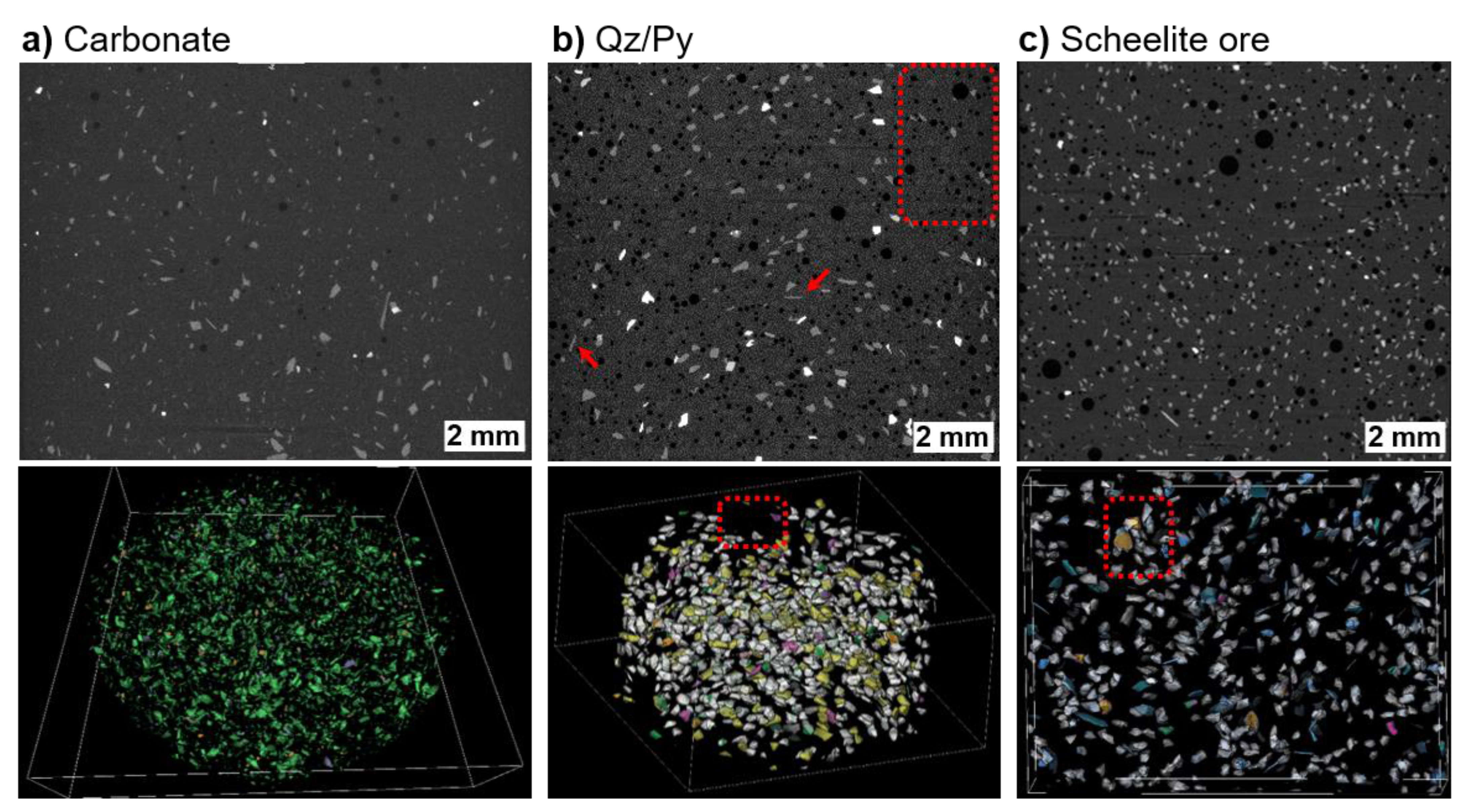
2.4.1. Carbonate Sample

The material used to prepare the Carbonate sample consists of particles with a size fraction of 100–500 µm that resulted from crushing and sieving a rock specimen originated in the Snowbird deposit, Montana, Canada [40]. The material consists of a carbonate matrix with embedded grains of parisite and as later discovered using MLA, pyrite and the nickel phases jamborite (Ni,Fe(OH)_x), liebenbergite (Ni₂(SiO₄)), and millerite (NiS). The sample was prepared using sugar with different size fractions as spacer: 4 g of sugar 71–160 µm, 3 g of sugar 160–300 µm and 1 g of sample particles. The resin used was a fast-curing acrylic polymer commonly used for dental repair, Paladur (Kulzer, Mitsui Chemical Group). The particles of the target material together with the sugar were mixed with methylmethacrylate-copolymer powder in the mass ratio 1:1. The methylmethacrylate liquid resin was added to the solid mixture in the ratio 3 mL/10 g. The final paste was poured into a tube 12 mm diameter and then left to dry for one hour.

CT scanning conditions: the maximum X-ray energy was 150 keV, the X-ray power was 15 W, the exposure time was 2.7 s, the number of projections was 2141, the scanning time was about 98 min, the voxel size was 10 µm with binning 2x of the detector’s pixels and one 0.5 mm Cu filter was mounted at the source. The reconstructed CT value interval was [0, 11.2]. Image processing was performed in Dragonfly. Labelling of particles was performed using a deep learning model with 3D sensor architecture that was trained using 245610 voxels of which 41770 represented particles. Phase classification in the 3D image was based on mineralogical information from MLA but without a direct correlation between 2D and 3D images.

2.4.2. Qz/Py Sample

This material originates from a handpicked rock from the Buzwagi gold mine that was crushed and sieved to a particle size of 200–315 µm. The material composition is known, as this is usually the case for material originated in an active mine. The main phases are quartz and pyrite, and known minor phases (<6%) are chalcopyrite, muscovite, fluorite and calcite. Knowing the phases present allowed the simulation of their attenuation coefficient as a function of the X-ray energy using the NIST database (Figure S1). The sample was prepared using sugar and graphite with different size fractions as spacer: 4 g of sugar < 71 µm, 2 g of sugar 160–300 µm, 2 g of graphite 5–10 µm and 1 g of the particles to be analysed. The mixture of particles was mixed with epoxy resin by hand stirring gently for 10 min. The mass ratio of particles to resin was 1:1.2. The mixture was poured into a tube 12 mm diameter and then left to dry overnight.

CT scanning conditions: the maximum X-ray energy was 160 keV, the power was 15 W, the exposure time was 3.6 s, the number of projections was 1438, the scanning time was about 88 min, the voxel size was 10 µm with binning 2x of the detector’s pixels and one 0.5 mm Cu filter was mounted at the source. The reconstructed CT value interval was [0, 26]. Using these scanning conditions, the effective energy was calculated from the measured transmission spectrum (Figure S2) using a spectral detector [38]. Image processing was achieved using Avizo. First, a non-local means image filter [41] with search window 17, local neighbourhood 3 and similarity 3 was applied to the raw data. Individual particles were segmented using a direct threshold value of 1100 followed by a marker-based watershed particle separation method [42] using H-maxima of 2 as defined in reference [35]. To reduce noise, a soft Kuwahara image filter was applied in FIJI to the grey-scale image three times, using the parameter window 1, before analysing the particle histograms. Phase classification was based on the X-ray attenuation coefficients at the calculated effective energy.

2.4.3. Scheelite Ore

The material belongs to the K1 ore body in the western ore zone of the Felbertal scheelite-deposit in the central Eastern Alps in Austria. The main phases in the K1-gneiss are quartz, feldspar and mica, and the minor phases include epidote, chlorite, calcite, sheelite, pyrite, chalcopyrite and pyrrhotite. Sample preparation for CT analysis used a particle size fraction of 200–150 µm. The sample was prepared using polymethyl metacrylate (PMMA) and graphite with different size fractions as spacer. Amounts of sample and spacer were measured volumetrically: 0.6 mL of the particles to be analysed (ca. 0.55 g, 14%), 1.4 mL graphite (ca. 0.30 g, 8%), 1.2 mL of PMMA < 71 µm size fraction (ca. 0.58 g, 15%), 2.4 mL of PMMA 160–71 µm size fraction (ca. 1.23 g, 32%) and 2.4 mL of PMMA 315–160 µm size fraction (ca. 1.23 g, 32%). The mixture of particles was blended with 2.84 g of Epotek epoxy resin by hand stirring gently for 10 min. The mixture was poured into a tube 16 mm diameter and then left to dry overnight.

CT scanning conditions: the maximum X-ray energy was 160 keV, the X-ray power was 15 W, the exposure time was 2.2 s, the number of projections was 2154, the scanning time was about 81 min, the voxel size was 12 µm with binning 2x of the detector’s pixels and one 0.2 mm Cu filter was mounted at the source. The reconstructed CT value interval was [0, 30]. Image analysis was performed in dragonfly. Labelling of particles was achieved using a deep learning model with 3D sensor architecture that was trained using 958422 voxels of which 45873 represented particles. Phase classification was based on the direct correlation of the sample’s cross-section in the 3D image and the corresponding 2D slice where the phases were classified by MLA.

3. Results

3.1. Sample Preparation

Vertical cross-sections of the three samples show that particles are randomly dispersed throughout the volume of the samples (Figure 2). The Carbonate sample (prepared using Paladur and without graphite,

Table 1. Summary of the types of material used to prepare the three samples analysed. The ParVox is defined as the middle value of the particle size fraction divided by the voxel size.

Material	Main Minerals	Sample Size (µm)	Particles Size Fractions (mass ratios)	# Particles/Volume (particles·mm−3)	ParVox
Carbonate	Parisite Millerite Pyrite Liebenbergite Jamborite Carbonate	100–500	Material 13%; Sugar: 71–160 µm (50%), 160–300 µm (37%)	20.3	25
Qz/Py	Chalcopyrite Pyrite Fluorite/Epidote Calcite Muscovite Quartz	315–425	Material 12%; Sugar: <71 µm (44 %), 160–315 µm (22%); Graphite: 5–10 µm (22%)	6.7	36
Scheelite ore	Scheelite Sulphides Epidote/Chlorite Calcite Mica Feldspar Quartz	150–200	Material 14%; PMMA: <71 µm (15 %), 160–71 µm (32%), 315–160 µm (32%); Graphite: 5–10µm (8%)	14.7	15

) has fewer bubbles and the particles are better separated than the particles in the samples prepared with epoxy resin and graphite. The Qz/Py sample shows some subvolumes with fewer particles (red box, Figure 2b), although the overall dispersion along the horizontal cross-section is similar. The poorer dispersion of the particles is possibly a result of the overall larger particle sizes that are not as easy to mix with the spacer as smaller particles. The presence of these areas did not have a measurable impact on the distribution of grey-values along the sample’s diameter. Additionally, the majority of particles are separated with few exceptions visible in the 2D section. The Scheelite ore sample shows mostly well dispersed particles, but several clusters of particles appear to touch each other (red box, Figure 2c). One factor that can contribute to this appearance is the lower particle size to voxel size ratio (ParVox) relatively to the other samples. From the three samples, the Carbonate sample is the closest to the ideal sample described earlier, since it provides a higher number of particles per volume (Table 1) while maintaining the separation between particles and a consistent dispersion throughout the sample’s volume. All samples show the presence of bubbles (black circles, Figure 2) that appear to be well dispersed and to contribute to create space between particles.

The histograms of the 3D images of each particulate material scanned without sample preparation, i.e., as packed particles in a tube (dotted lines, Figure 3), and as particle dispersions, i.e., prepared according to MSPaCMAn (dashed lines, Figure 3), are compared relative to the ability to distinguish different phases. Additionally, those histograms from the whole image are compared to the histograms of individual particles after applying the MSPaCMAn workflow (continuous lines for which colours correspond to different particles, Figure 3). Typically, a phase can only be classified if it is represented by a recognizable peak at a specific position in the histogram. Since the histograms of the packed particle samples show broad bands instead of individual peaks it can be assumed that only few phases or actually groups of phases could be distinguishable. On the other hand, the histogram of samples that were prepared using a particle dispersion show narrower bands, some of which differentiate into individual peaks that correspond to specific phases. Despite the improvement, many of the bands are seen to overlap with each other, thus an incorrect classification of voxels would still be expected if segmentation is performed by applying a grey-scale threshold to the entire image.

As an alternative to whole image analysis, since the particles are labelled individually using the MSPaCMAn workflow, the histogram of each particle can be analysed independently. The histograms of individual particles show peaks (continuous lines, Figure 3) that are better defined than in the histograms corresponding to the whole sample. Some peaks of different particles show partial overlap (e.g., particles 2 and 3, Figure 3a; and particles 1, 2 and 3, Figure 3c); however, the grey-values at the maximum of the peak can be distinguished and used to classify the phase corresponding to the entire peak. The widths of the peaks in a sample seem to be related to the ParVox (Table 1), i.e., peaks are sharper for the Qz/Py sample (ParVox 36), and peaks are wider and noisier for the Sheelite ore (ParVox 15). The peak classification criteria will be discussed for each sample individually.

3.2. Phase Classification in Individual Particles

To highlight the advantages of using individual particle histograms to classify the phases in a material, a different strategy was used to analyze each material: the Carbonate sample was classified based on MLA characterization but without a direct correlation between images; the Qz/Py sample was classified using the X-ray attenuation coefficient of the phases known to be present; and the Scheelite ore sample was classified based on the direct correlation of the sample’s cross-section in the 3D image and the corresponding slice analyzed by MLA as well as using the geometrical properties of the particles.

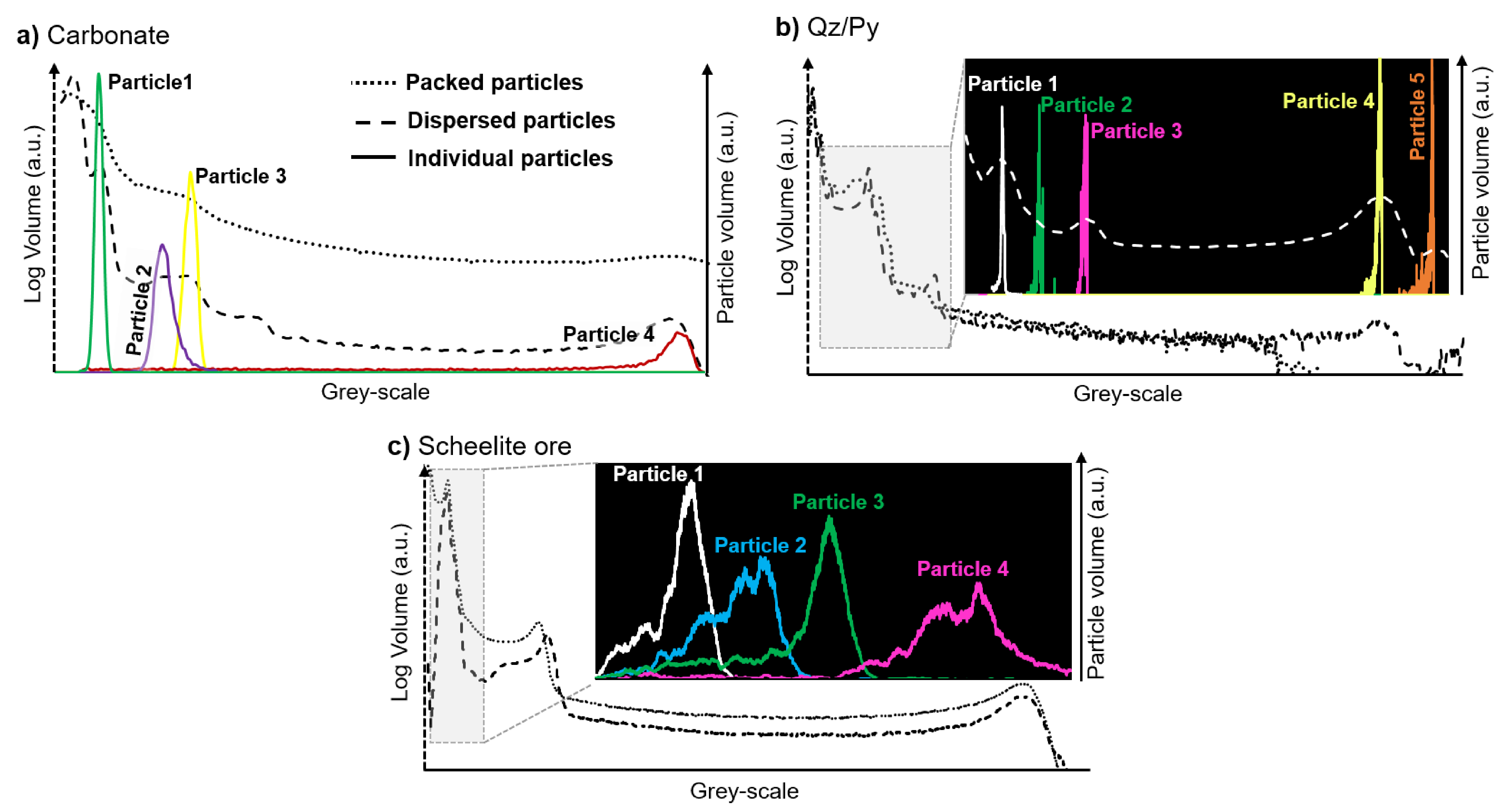
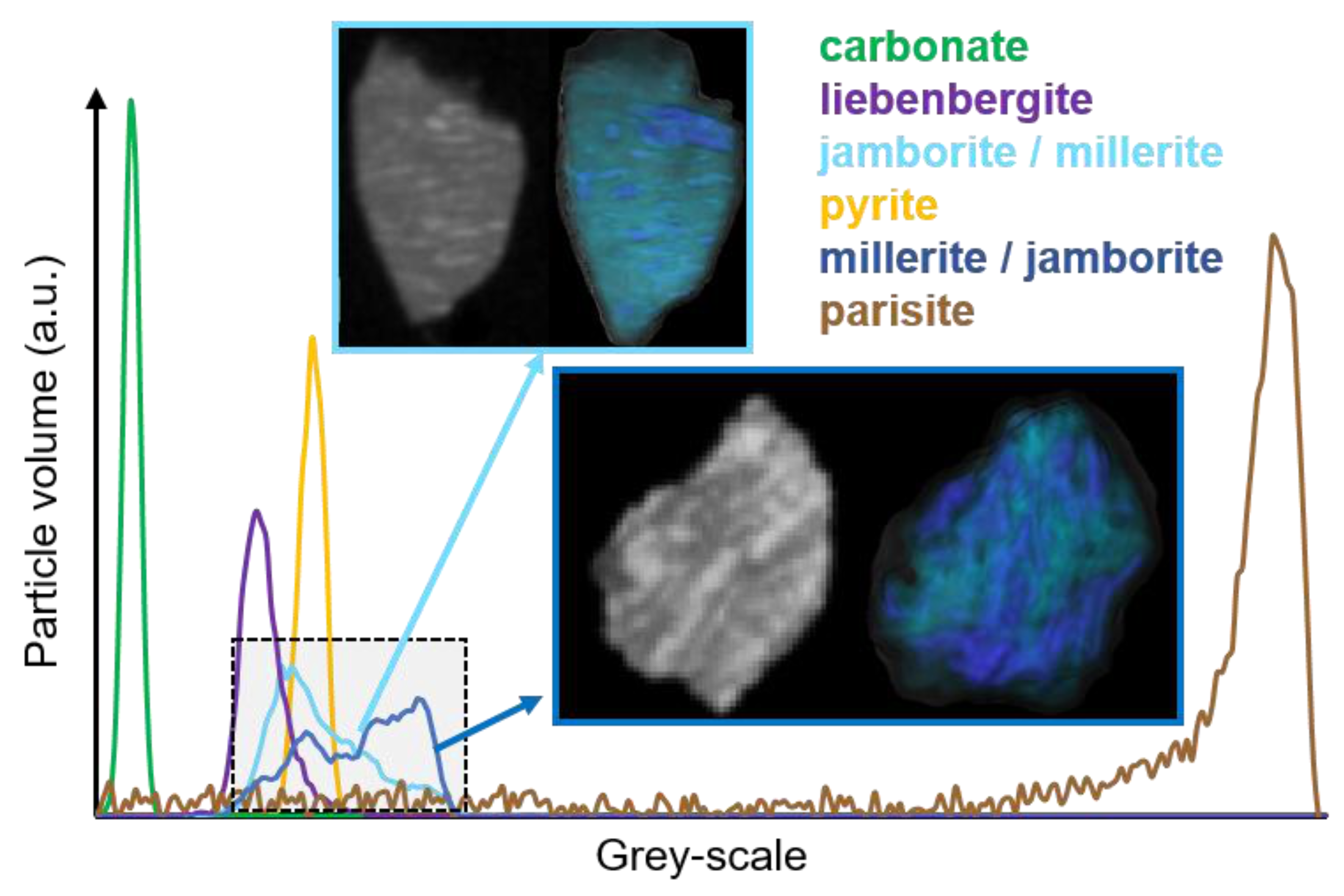
3.2.1. Carbonate Sample

The MLA analysis shows that the sample is mainly composed of dolomite (CaMg(CO₃), 28%, density 2.7 g·cm⁻³), calcite (Ca(CO₃), 66.8%, density 2.8 g·cm⁻³), pyrite (FeS 2.3%, density 5 g·cm⁻³), parisite (0.9%, density 4.4 g·cm⁻³) and three phases containing nickel, jamborite (Ni,Fe(OH)_x, 0.6%, density 2.7 g·cm⁻³), liebenbergite Ni(SiO₄), 0.9%, density 4.6 g·cm⁻³) and millerite (NiS, 0.5%, density 5.5 g·cm⁻³). The different minerals are mostly liberated (within the resolution of CT), except jamborite and millerite that always occur as intergrown microstructures (light and dark blue, Figure 4). Calcite and dolomite are also frequently associated.

Several phases identified by MLA could be distinguished on individual particle histograms by the characteristic peaks (Figure 5). The exception was dolomite and calcite that have similar attenuation coefficients, and thus are classified as the carbonate group (green peak). Particles containing parisite show the broadest main peak (brown line) and a significant number of minor peaks throughout the grey-scale. The minor peaks are attributed to scattering artefacts and partial volume effect that can affect the grey-values of voxels at the edges of phases with high attenuation. Particles with the joint jamborite-millerite microstructure show a characteristic continuous band that may exhibit one or two main peaks with variable intensity, depending on which of the two phases is dominant in the particle (blue lines). This is exemplified by two particles in Figure 5, one particle has higher content of jamborite (light blue) and the second particle has higher content of millerite (dark blue). The higher the content of jamborite, the more pronounced is the left side of the band as opposed to higher contents of millerite that are reflected by higher frequencies at the right side of the band (compare blue lines, Figure 5). The position of the peak’s maximum may vary depending on the size of the grains within the particle. Based on the attenuation coefficients of the pure minerals (if grains are sufficiently large relative to the voxel size), it would be expected that the peak position of jamborite is between liebenbergite (purple line) and carbonate (green line). Note that the peaks of pyrite and liebenbergite particles already partially overlap; thus, it would be impossible to distinguish the peak of jamborite in the present microstructure with millerite without an individual particle analysis. Nevertheless, the presence of jamborite in a particle can be identified by the characteristic bands that identify the intergrown with millerite (highlighted in the grey box, Figure 5). In conclusion, using MSPaCMAn it is possible to distinguish the three nickel phases and pyrite, which would be futile using traditional whole image threshold-based classification. Note that the interpretation of microstructures must rely on preexisting mineralogical data. In this case, the criteria used to classify jamborite and millerite rely on the observation that both phases are associated and none of them are associated with pyrite.

3.2.2. Qz/Py Sample

Preliminary knowledge about the mineralogy of the Buzwagi mine, and the calculated effective energy of the scan (E_eff = 72.8 keV, Figure S2) allowed to predict the relative positions of the peaks of each mineral phase present in the material. The proximity of the attenuation coefficients of pyrite and chalcopyrite, and of quartz and muscovite anticipates a challenge to distinguish the phases (Figure S1). This is confirmed by the absence of differentiated peaks corresponding to these phases in the whole image histograms, Figure 3b. Nevertheless, using MSPaCMAn, the position of the peaks of individual particles is clearly distinguishable. The overlap of individual particle histograms with the plot of the attenuation coefficient as a function of the X-ray energy at 72.8 keV shows a good match of the maximum of each peak with the theoretical values of the attenuation coefficients of the corresponding phase, Figure 6. Muscovite shows the broadest peak, which can be attributed to the higher number of voxels affected by PVE representing flat shaped particles (red arrows in Figure 2b). The other phases are represented by peaks significantly narrower than the peaks visible in the histogram of the other two samples (Figure 3). This is attributed to the overall larger particle sizes of the Qz/Py sample.

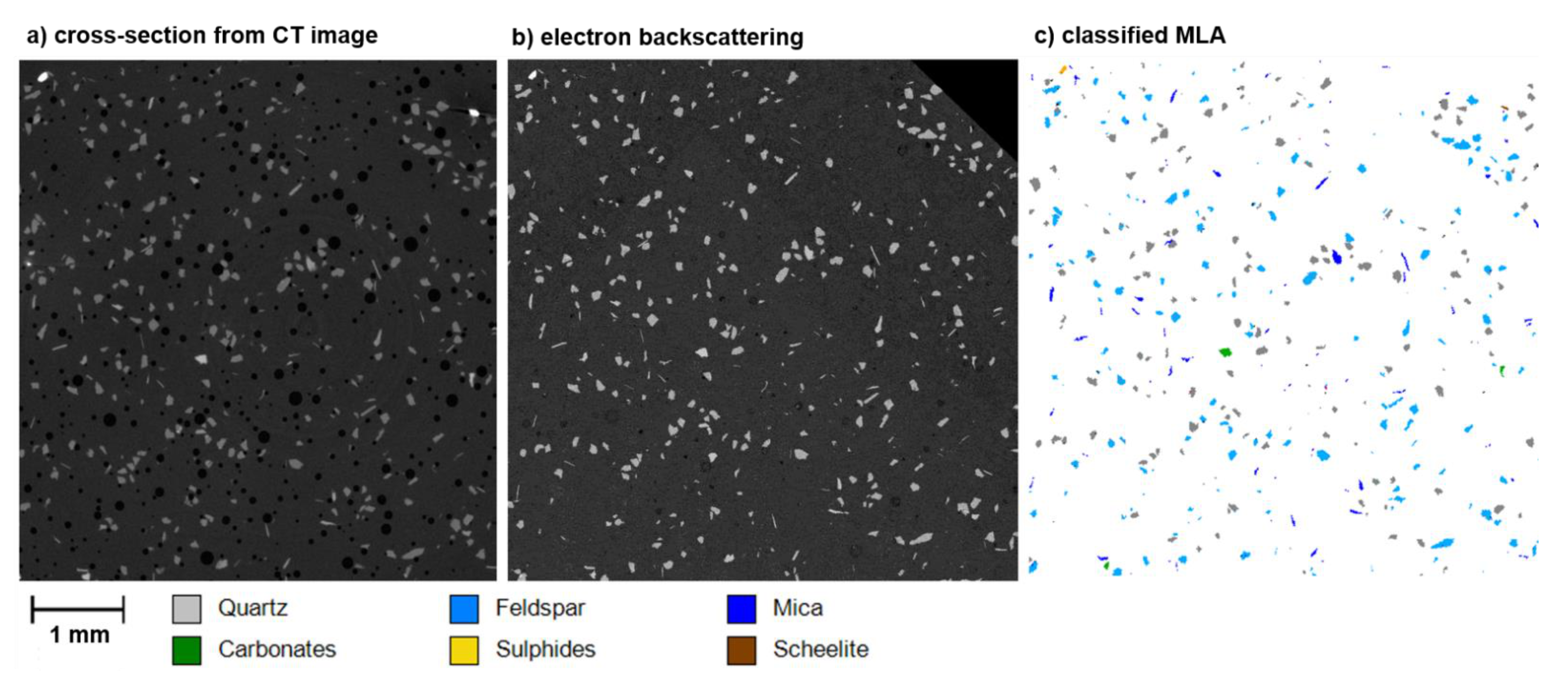
3.2.3. Scheelite Ore Sample

In contrast to the carbonate and the Qz/Py samples, the Scheelite ore is known to be composed of phases that may have variable chemical composition (e.g., feldspar groups). In such cases it would be difficult to estimate a theoretical attenuation coefficient of a phase, similar to what was done for the Qz/Py sample. Thereafter, the position of the peak of each phase or each mineral group was determined by the direct correlation of the sample’s cross-section in the 3D image and the corresponding slice analyzed by MLA. The MLA showed a presence of mainly quartz (42.5%), feldspar (38.7%) and mica (13.9%), and minor minerals such as pyrite, chalcopyrite and pyrrhotite that are mostly associate and were grouped as sulfides (1.3%), epidote and chlorite that are typically associated (1%), carbonates (0.6%) and scheelite (0.4%).

The scheelite is clearly distinguishable from the other phases due to its higher attenuation (brown line, Figure 7). Similar to the parisite in the Carbonate sample (Figure 5), the high attenuation of scheelite causes imaging artefacts, which are expressed as minor peaks throughout the grey-scale. Iron and copper sulphide phases could not be distinguished due to the similar attenuation and common association between these phases, thus they must be considered as a mineral group (orange line). Epidote and chlorite are typically associated with each other and to other minerals within the same particle (Figure S3), which results in broader multiple peaks in the histogram (pink line, at least two peaks). This makes the presence of these multiphase particles identifiable but difficult to distinguish between the phases within the particle. In comparison with the Qz/Py sample, the peaks are broader and all particles exhibit more minor peaks on the left side of the main peak. This is associated to the lower ParVox used to analyze this sample (Table 1), which increases the contribution of partial volume effect and spot blurriness to form minor peaks in a particle’s histogram [23].

Mica (blue) and feldspar (yellow) are undistinguishable based on the interval of grey-values characteristic of the maximum of the main peaks. Nevertheless, since the minerals occur mostly as liberated particles the two phases were distinguished based on the characteristic geometrical properties of the particles. In this case, mica has a distinct plate-like shape as opposed to the more spheroidal shape of feldspar (Figure 8). The characteristic shape descriptor of the particles can be calculated based on different geometrical parameters that are measured directly from the 3D image of a particle. The ratio between the minimum orthogonal distance between two points in a particle that pass through its center and the maximum Feret diameter (O_min/F_max) was measured in Dragonfly for 10 mica, 9 quartz and 9 feldspar particles visible at the cross-section where the mineral in each particle has been identified by MLA (e.g., Figure 9). The variability of O_min/F_max measured for each phase are shown in a box plot (Figure 8), where the boxes delimit the first and third quartile, the whiskers delimit the maximum and minimum values, and the horizontal line inside each box marks the median value. Since the range of O_min/F_max values of mica particles does not overlap with the range of O_min/F_max values of feldspar and quartz particles, this geometrical property can be used in addition to the grey-scale criteria to classify liberated mica particles. No significant geometrical difference between quartz and feldspar particles could be found that could assist in the phase classification of the partially overlapping peaks of the two phases (grey and yellow, Figure 7). Despite the significant overlap, the positions of the peak’s maximums corresponding to quartz or to feldspar are consistently different, and thus sufficient to distinguish the two phases.

4. Discussion

MSPaCMAn is founded on two interconnected ideas: (1) optimized sample preparation of particle dispersions reduces imaging artefacts and eases the segmentation of individual particles; (2) phase classification is performed at the particle level, which simplifies the interpretation of the grey-scale and allows adding particle- and phase-specific properties as classification criteria. Using a particle-based phase classification, the workflow proposed here is demonstrated to allow differentiating between phases that would not be distinguishable using conventional CT image analysis. The different steps of the workflow are shown to be adjustable to the specific particle system. Next, the advantages, limitations and further improvements of the different steps are discussed.

4.1. Sample Preparation

The preparation of particle dispersions was demonstrated to be a key enabler of the new method. First, the more consistent distribution of particles throughout the sample makes beam hardening similar at all positions of the sample. This is a requirement to allow the comparison of the grey-values of different particles, e.g., the grey-value that identifies a phase (main-peak position in a histogram) is independent from the position of the particle within the sample. Second, the labelling of thousands of individual particles can be achieved with minimum image processing, which is only possible due to the distancing between the sample’s particles imposed by “X-ray invisible” spacers. The ease of image processing is a requirement for the future development of semi-automated 3D mineralogical characterization.

The different types of spacer, of embedding materials and of particles to be analysed regarding composition and particle size tested in this work to prepare the particle dispersions demonstrates the versatility of the method. Note that the conditions used to prepare each sample are not optimized, but can serve as reference points to further optimization that can promote ideal particle dispersions. For instance, when scanning a material with ParVox of about 15 (as used for the Sheelite ore, Table 1) a smaller percentage of target material relative to the spacer should be considered in order to promote distancing between particles. Due to the small particle size in the sample, increasing the amount of the spacer size fraction <71 μm relative to the size fraction 160–315 μm could also promote the separation of particles. Furthermore, optimization of the size of the spacer to promote a distribution of larger particles better than that achieved for the Qz/Py sample would be recommended; for example, by substituting the graphite fraction by a spacer with particle sizes in the range of the sample’s particle size (315–425 μm). Using Paladur as embedding material seems to benefit particle separation while at the same time maintaining a high number of particles per volume of sample (Table 1). This could possibly be related to the observed decrease of the amount of air bubbles in the sample that may contribute to a more efficient use of the sample’s volume to disperse the particles (Figure 2).

The improved definition of the peaks in the histogram of 3D images of the material simply due to the sample preparation is clear (Figure 3). This improvement can be attributed to the decrease of the amount of voxels at the interphase between particles; for example, considering a simple system with particles of phase P1 or P2, and a background B. Without sample preparation, particles would touch each other producing five types of interphases, each with a specific gradient of grey-values: P1-B, P1-P1, P1-P2, P2-B and P2-P2. In an ideal particle dispersion, the particles do not touch each other; thus, only two types of interphases are expected: P1-B and P2-B. The benefit is even more prominent for materials with more phases. Reducing the type of interphases reduces the number of minor peaks that are not characteristic of specific phases, which simplifies the histogram analysis. This simplification opens the opportunity to interpret histogram signals that are specific of an interphase to analyse mineral associations or to detect specific microstructures bellow the spatial resolution of the scan (Figure 5). It can be concluded that scanning particle dispersions, even non-ideal, improves the contrast resolution between phases, i.e., shortens the minimum difference between attenuation coefficients (or peak positions) that can be distinguished as independent phases.

4.2. Individual Particle Analysis

The distance between particles, enlarged by the sample preparation, facilitates the segmentation and labelling of individual particles. That means the entire image can be broken-down into smaller and independent regions (one per particle) with a comparable grey-scale (also as a result of the sample preparation). The histogram of individual particles is significantly simplified relative to the entire sample (Figure 3), which allows distinguishing phases that cannot be recognized using whole image analysis methods. In practice, individual particle analysis enables the optimization of phase classification to less complex volumes and the establishment of classification criteria (not restricted to the grey-values) that are specific to each particle, e.g., particle size, shape, mineral associations and any other preliminary knowledge about the material.

First, the image is processed to segment the particles. The best segmentation strategy is intrinsically related to the ParVox. Due to the larger ParVox used to analyze the Qz/Py sample (Table 1), segmentation could be achieved using a simple grey-scale threshold method to differentiate particles from background. Alternatively, deep learning segmentation was found to be more accurate to segment particles with lower ParVox and with large grains of high density phases such as parisite and scheelite since it reduces the over segmentation caused by image artefacts.

Segmentation may fail to identify all particles in a sample due to inevitable deviations from the ideal particle dispersion that lead to some contact between particles. This is visible in the Qz/Py sample that has a more heterogeneous particle dispersion, and in the Scheelite ore sample that formed some particle agglomerates that were not separated by the spacer. To separate the over-segmented regions into individual particles, it was necessary to apply a watershed separation method. The success of separating particles using watershed is higher for higher ParVox [35]. Therefore, a better separation was achieved for the Qz/Py sample, while only partial separation could be achieved for the Scheelite ore sample. In conclusion, image processing allows correction for deviations from the ideal sample preparation and can be added or removed to the workflow to improve the accuracy of segmenting individual particles. This represents a simplification relative to traditional image processing strategies that aim at segmenting individual grains (smaller than particles). Using MSPaCMAn, grains do not need to be segmented since phase analysis is performed using a particle-based interpretation of the grey-values of all voxels in the particle.

4.3. Phase Classification

Once the particles have been labeled with a unique identifier, their constituent phases can be classified by applying a set of classification criteria to each particle. These classification criteria can be of two types: based on geometrical properties of the particle and based on the histogram that represents the grey-values of all voxels in the particle. Defining the specific criteria to classify the phases in a particulate material requires preliminary knowledge about the sample. For instance, it is imperative to know which phases are present as large grains, i.e., significantly larger than the voxel size. Such grains are represented by main-peaks with a maximum at grey-values that are specific of a phase, thus can be used as classification criteria. Since the maximum of peaks is within intervals of grey-values narrower than the entire peak, even if two peaks partially overlap, the phases could be distinguished, e.g., quartz and feldspar, Figure 7.

Tagging a specific interval of grey-values to a specific phase can be achieved using a relative scale of the X-ray attenuation coefficients of all phases expected in the sample. This can be easily performed for samples with relatively simple and well known mineralogy such as the Qz/Py sample, or for samples with a small number of phases such as the Carbonate sample. In fact, the demonstrated match of the relative peak positions with the theoretical X-ray attenuation coefficients endorses the idea that some phases could be identified even without preliminary knowledge. Nevertheless, if a sample is composed of complex minerals that may present a variable chemical composition, thus without a single the attenuation coefficient, a calibration of the grey-values for each phase is necessary. For example, the direct correlation with 2D image-based mineralogical methods allows organising the phases into mineral groups with similar X-ray attenuation coefficients using the chemical information measured with the 2D method. However, such correlative methods are time consuming and impractical to be implemented as part of a semi-automated method.

Grains with sizes close to or smaller than the voxel size can make the interpretation of the histograms challenging. Nevertheless, MSPaCMAn shows that if it is known that a specific microstructure gives a recognizable signal in the histogram (e.g., intergrown jamborite and millerite, Figure 5) then the phases may still be identifiable and possibly quantifiable. Knowledge about the specific geometry of particles containing a phase can also be used as criteria to define the phase. Such criteria can be combined hierarchically after grey-value criteria. For example, for peaks with the maximum frequency of grey-values within a specific grey-scale interval (e.g., within the dark-grey box that comprise the peaks of feldspar and mica, Figure 7), if particles have a shape factor bellow a specified value (red region, Figure 8), then it is classified as mica, else it is feldspar. Additional criteria can be add or removed such hierarchical classification depending on the complexity of the sample. It is expected that the classification accuracy would increase with the amount of preliminary information about the material that results in more selective criteria.

4.4. Applications and Further Developments

The cases presented in this work mostly refer to liberated grains (one phase per particle) or to microstructures easy to identify. Nevertheless, it is anticipated that more challenging materials with multiple phases per particle could also be more accurately characterized using MSPaCMAn than using conventional CT analysis methods. That is because the histogram of individual particles would always be simpler than the whole image histogram. Nevertheless, the full scope of applicability of the workflow to distinguish multiple phases in a particle (peaks in a histogram) and the quantification of a phase based on the histogram analysis are yet to be tested. It should be noted that the benefits of the method come from the simplification of the microstructures inside individual particles relative to the microstructures found if the particles were assembled as one structure, e.g., as a rock or as non-separated particles. Additional benefits arise from the more homogeneous distribution of those microstructures in the particulate sample relative to the more asymmetric textures found in rocks that cause imaging artefacts. Therefore, the larger the particles and the less liberated the grains are, the lesser the benefit from using our method.

Four key developments should be considered in order to universalize the new workflow for the standardized characterization of particulate materials:

(1)

To develop a systematic sample preparation procedure where the size of the spacer and the embedding material is determined by the size fraction of the sample’s particles.

(2)

To build a database for the hierarchical implementation of the selective criteria that can be used to classify a mineral, a group of minerals and/or the specific minerals and microstructures of a particular deposit. This could include developing a database of reference peak positions corresponding to a mineral. For instance, 2D/3D correlative methods could be used to classify specific phases in the 3D image of a reference material and stored as a database to be called every time another system with a similar composition is analyzed.

(3)

To automate the phase classification, by applying a set of defined criteria to all the particles.

(4)

To derive a particle/histogram-based method to quantify the mineralogical information contained in the histograms of the individual particles, which can be extrapolated to all particles in a sample. If these four developments can be realized, MSPaCMAn could be the foundation of semi-automated quantitative 3D mineral characterization methods.

5. Conclusions

A new workflow, MSPaCMAn, is demonstrated to ease the classification of phases composing particulate materials with high phase resolution. Scanning samples prepared as particle dispersions is shown to yield a comparable grey-scale throughout the sample and to ease the segmentation of individual particles. This allows the implementation of particle-specific criteria to classify its constituent phases, which makes it possible to distinguish between phases with similar X-ray attenuation coefficients, i.e., represented by similar voxel grey-values in the 3D image. The improved ability to classify particles results from the simplified grey-scale description of individual particles (e.g., as a histogram) relative to the complex grey-scale description of the entire image. Additionally, particle-based classification allows use of the properties of a particle (e.g., geometrical and mineralogical properties) as part of the classification criteria (i.e., beyond the grey-values). The ability to distinguish phases with similar X-ray attenuation with an improved accuracy can be the starting point of more comprehensive quantitative 3D mineral characterization techniques. Such a method would be a unique source of 3D particle information that could be used to interpret, predict and optimize particle processing methods used by the raw materials industry.

6. Patents

The idea behind the work described in this paper has been filed for patenting and awaits revision [32].

References

1. The Role of Critical Minerals in Clean Energy Transitions; International Energy Agency: Paris, France. 2021. Available online: https://iea.blob.core.windows.net/assets/24d5dfbb-a77a-4647-abcc-667867207f74/TheRoleofCriticalMineralsinCleanEnergyTransitions.pdf (accessed on 2 August 2021).
2. Ueda, T.; Oki, T.; Koyanaka, S. Experimental analysis of mineral liberation and stereological bias based on X-ray computed tomography and artificial binary particles. Adv. Powder Technol. 2018, 29, 462–470. [Google Scholar] [CrossRef]
3. Reyes, F.; Lin, Q.; Cilliers, J.J.; Neethling, S.J. Quantifying mineral liberation by particle grade and surface exposure using X-ray microCT. Miner. Eng. 2018, 125, 75–82. [Google Scholar] [CrossRef]
4. Blannin, R.; Frenzel, M.; Tuşa, L.; Birtel, S.; Ivăşcanu, P.; Baker, T.; Gutzmer, J. Uncertainties in quantitative mineralogical studies using scanning electron microscope-based image analysis. Miner. Eng. 2021, 167, 106836. [Google Scholar] [CrossRef]
5. Pereira, L.; Frenzel, M.; Khodadadzadeh, M.; Tolosana-Delgado, R.; Gutzmer, J. A self-adaptive particle-tracking method for minerals processing. J. Clean. Prod. 2021, 279, 123711. [Google Scholar] [CrossRef]
6. Schach, E.; Buchmann, M.; Tolosana-Delgado, R.; Leißner, T.; Kern, M.; van den Gerald Boogaart, K.; Rudolph, M.; Peuker, U.A. Multidimensional characterization of separation processes—Part 1: Introducing kernel methods and entropy in the context of mineral processing using SEM-based image analysis. Miner. Eng. 2019, 137, 78–86. [Google Scholar] [CrossRef]
7. Parian, M.; Lamberg, P.; Rosenkranz, J. Developing a particle-based process model for unit operations of mineral processing—WLIMS. Int. J. Miner. Process. 2016, 154, 53–65. [Google Scholar] [CrossRef]
8. Buchmann, M.; Schach, E.; Leißner, T.; Kern, M.; Mütze, T.; Rudolph, M.; Peuker, U.A.; Tolosana-Delgado, R. Multidimensional characterization of separation processes—Part 2: Comparability of separation efficiency. Miner. Eng. 2020, 150, 106284. [Google Scholar] [CrossRef]
9. Furat, O.; Leißner, T.; Bachmann, K.; Gutzmer, J.; Peuker, U.; Schmidt, V. Stochastic Modeling of Multidimensional Particle Properties Using Parametric Copulas. Microsc. Microanal. 2019, 25, 720–734. [Google Scholar] [CrossRef] [Green Version]
10. Hoang, D.H.; Kupka, N.; Peuker, U.A.; Rudolph, M. Flotation study of fine grained carbonaceous sedimentary apatite ore—Challenges in process mineralogy and impact of hydrodynamics. Miner. Eng. 2018, 121, 196–204. [Google Scholar] [CrossRef]
11. Buchmann, M.; Schach, E.; Tolosana-Delgado, R.; Leißner, T.; Astoveza, J.; Kern, M.; Möckel, R.; Ebert, D.; Rudolph, M.; van den Boogaart, K.; et al. Evaluation of Magnetic Separation Efficiency on a Cassiterite-Bearing Skarn Ore by Means of Integrative SEM-Based Image and XRF–XRD Data Analysis. Minerals 2018, 8, 390. [Google Scholar] [CrossRef] [Green Version]
12. Guntoro, P.I.; Ghorbani, Y.; Koch, P.-H.; Rosenkranz, J. X-ray Microcomputed Tomography (µCT) for Mineral Characterization: A Review of Data Analysis Methods. Minerals 2019, 9, 183. [Google Scholar] [CrossRef] [Green Version]
13. Withers, P.J.; Bouman, C.; Carmignato, S.; Cnudde, V.; Grimaldi, D.; Hagen, C.K.; Maire, E.; Manley, M.; Du Plessis, A.; Stock, S.R. X-ray computed tomography. Nat. Rev. Methods Primers 2021, 51, 1–21. [Google Scholar] [CrossRef]
14. Reyes, F.; Lin, Q.; Udoudo, O.; Dodds, C.; Lee, P.D.; Neethling, S.J. Calibrated X-ray micro-tomography for mineral ore quantification. Miner. Eng. 2017, 110, 122–130. [Google Scholar] [CrossRef] [Green Version]
15. Miller, J.D.; Lin, C.L. X-ray tomography for mineral processing technology 3D particle characterization from mine to mill. Miner. Metall. Process. 2018, 35, 1–12. [Google Scholar] [CrossRef]
16. Miller, J.D.; Lin, C.-L.; Hupka, L.; Al-Wakeel, M.I. Liberation-limited grade/recovery curves from X-ray micro CT analysis of feed material for the evaluation of separation efficiency. Int. J. Miner. Process. 2009, 93, 48–53. [Google Scholar] [CrossRef]
17. Furat, O.; Leißner, T.; Ditscherlein, R.; Šedivý, O.; Weber, M.; Bachmann, K.; Gutzmer, J.; Peuker, U.; Schmidt, V. Description of Ore Particles from X-Ray Microtomography (XMT) Images, Supported by Scanning Electron Microscope (SEM)-Based Image Analysis. Microsc. Microanal. 2018, 24, 461–470. [Google Scholar] [CrossRef] [PubMed]
18. Wang, Y.; Lin, C.L.; Miller, J.D. Quantitative analysis of exposed grain surface area for multiphase particles using X-ray microtomography. Powder Technol. 2017, 308, 368–377. [Google Scholar] [CrossRef]
19. Guntoro, P.I.; Ghorbani, Y.; Parian, M.; Butcher, A.R.; Kuva, J.; Rosenkranz, J. Development and experimental validation of a texture-based 3D liberation model. Miner. Eng. 2021, 164, 106828. [Google Scholar] [CrossRef]
20. Bauer, C.; Wagner, R.; Orberger, B.; Firsching, M.; Ennen, A.; Garcia Pina, C.; Wagner, C.; Honarmand, M.; Nabatian, G.; Monsef, I. Potential of Dual and Multi Energy XRT and CT Analyses on Iron Formations. Sensors 2021, 21, 2455. [Google Scholar] [CrossRef]
21. Boas, F.E.; Fleischmann, D. CT artifacts: Causes and reduction techniques. Imaging Med. 2012, 4, 229–240. [Google Scholar] [CrossRef] [Green Version]
22. Lin, Q.; Neethling, S.J.; Dobson, K.J.; Courtois, L.; Lee, P.D. Quantifying and minimising systematic and random errors in X-ray micro-tomography based volume measurements. Comput. Geosci. 2015, 77, 1–7. [Google Scholar] [CrossRef] [Green Version]
23. Godinho, J.R.A.; Kern, M.; Renno, A.D.; Gutzmer, J. Volume quantification in interphase voxels of ore minerals using 3D imaging. Miner. Eng. 2019, 144, 106016. [Google Scholar] [CrossRef]
24. Pankhurst, M.J.; Fowler, R.; Courtois, L.; Nonni, S.; Zuddas, F.; Atwood, R.C.; Davis, G.R.; Lee, P.D. Enabling three-dimensional densitometric measurements using laboratory source X-ray micro-computed tomography. SoftwareX 2018, 7, 115–121. [Google Scholar] [CrossRef]
25. Voigt, M.; Miller, J.A.; Mainza, A.N.; Bam, L.C.; Becker, M. The Robustness of the Gray Level Co-Occurrence Matrices and X-Ray Computed Tomography Method for the Quantification of 3D Mineral Texture. Minerals 2020, 10, 334. [Google Scholar] [CrossRef] [Green Version]
26. Godinho, J.R.A.; Westaway-Heaven, G.; Boone, M.A.; Renno, A.D. Spectral Tomography for 3D Element Detection and Mineral Analysis. Minerals 2021, 11, 598. [Google Scholar] [CrossRef]
27. Ditscherlein, R.; Leißner, T.; Peuker, U.A. Preparation techniques for micron-sized particulate samples in X-ray microtomography. Powder Technol. 2020, 360, 989–997. [Google Scholar] [CrossRef]
28. Ditscherlein, R.; Furat, O.; de Langlard, M.; Martins de Souza E Silva, J.; Sygusch, J.; Rudolph, M.; Leißner, T.; Schmidt, V.; Peuker, U.A. Multiscale Tomographic Analysis for Micron-Sized Particulate Samples. Microsc. Microanal. 2020, 26, 676–688. [Google Scholar] [CrossRef] [PubMed]
29. Dougherty, E.R. Mathematical Morphology in Image Processing, 1st ed.; CRC Press: Boca Raton, FL, USA, 2018; ISBN 9781351830508. [Google Scholar]
30. Bam, L.C.; Miller, J.A.; Becker, M.; De Beer, F.C.; Basson, I. (Eds.) X-ray Computed Tomography—Determination of Rapid Scanning Parameters for Geometallurgical Analysis of Iron Ore. In Proceedings of the Third ausimm International Geometallurgy Conference, Perth, Australia, 15–16 June 2016. [Google Scholar]
31. Evans, C.L.; Napier-Munn, T.J. Estimating error in measurements of mineral grain size distribution. Miner. Eng. 2013, 52, 198–203. [Google Scholar] [CrossRef]
32. Godinho, J.R.A.; Pereira, L. A Method and Device for 3D Analyzes of a Particulate Material. EP 21 158 241.6. 16 February 2021. [Google Scholar]
33. Videla, A.R.; Lin, C.L.; Miller, J.D. 3D characterization of individual multiphase particles in packed particle beds by X-ray microtomography (XMT). Int. J. Miner. Process. 2007, 84, 321–326. [Google Scholar] [CrossRef]
34. Da Wang, Y.; Shabaninejad, M.; Armstrong, R.T.; Mostaghimi, P. Physical Accuracy of Deep Neural Networks for 2D and 3D Multi-Mineral Segmentation of Rock micro-CT Images. arXiv 2002, arXiv:2002.05322v2. [Google Scholar]
35. Alam, M.F.; Haque, A. A New Cluster Analysis-Marker-Controlled Watershed Method for Separating Particles of Granular Soils. Materials 2017, 10, 1195. [Google Scholar] [CrossRef] [PubMed] [Green Version]
36. Bam, L.; Miller, J.; Becker, M. A Mineral X-ray Linear Attenuation Coefficient Tool (MXLAC) to Assess Mineralogical Differentiation for X-ray Computed Tomography Scanning. Minerals 2020, 10, 441. [Google Scholar] [CrossRef]
37. Schulz, B.; Sandmann, D.; Gilbricht, S. SEM-Based Automated Mineralogy and Its Application in Geo- and Material Sciences. Minerals 2020, 10, 1004. [Google Scholar] [CrossRef]
38. Sittner, J.; Godinho, J.R.A.; Renno, A.D.; Cnudde, V.; Boone, M.; de Schryver, T.; van Loo, D.; Merkulova, M.; Roine, A.; Liipo, J. Spectral X-ray computed micro tomography: 3-dimensional chemical imaging. X-ray Spectrom. 2021, 50, 92–105. [Google Scholar] [CrossRef]
39. Warr, R.; Ametova, E.; Cernik, R.J.; Fardell, G.; Handschuh, S.; Jørgensen, J.S.; Papoutsellis, E.; Pasca, E.; Withers, P.J. Enhanced hyperspectral tomography for bioimaging by spatiospectral reconstruction. arXiv 2021, arXiv:2103.04796v1. [Google Scholar]
40. Samson, I.M.; Wood, S.A.; Finucane, K. Fluid Inclusion Characteristics and Genesis of the Fluorite-Parisite Mineralization in the Snowbird Deposit, Montana. Econ. Geol. 2004, 99, 1727–1744. [Google Scholar] [CrossRef]
41. Buades, A.; Coll, B.; Morel, J.M. A non-local algorithm for image denoising. In Proceedings of the 2005 IEEE Computer Society Conference on Computer Vision and Pattern Recognition (CVPR’05), San Diego, CA, USA, 20–25 June 2005; Volume 2, pp. 60–65. [Google Scholar]
42. Wang, Y.; Lin, C.L.; Miller, J.D. 3D image segmentation for analysis of multisize particles in a packed particle bed. Powder Technol. 2016, 301, 160–168. [Google Scholar] [CrossRef]
Figure 1. Scheme of the MSPaCMAn workflow. (a) Step 1, sample preparation and scanning; (b) Step 2, individual particle analysis; Step 3, (c) calculation of the geometrical properties of a particle, and (d) classification of the minerals in the sample.
Minerals 11 00947 g001
Figure 2. Overview of the CT results for the three samples (ac). On top, are vertical cross-sections of the sample, whereby bubbles are black and particles are grey-tones (brighter colors within each sample correspond to denser phases). On the bottom are 3D views of subvolumes within the sample: (a) 14 mm × 14 mm × 3 mm, (b) 14 mm × 14 mm × 6 mm, (c) 6 mm × 5 mm × 1.1 mm. Colors correspond to mineral groups of minerals with similar grey-values (independent grey-scale for each sample).
Minerals 11 00947 g002
Figure 3. Comparison of the histogram of 3D images corresponding to samples of the same material but scanned without sample preparation as packed particles (dotted line) and prepared as particle dispersions (dashed line), and the histogram of individual particles obtained by applying MSPaCMAn (continuous lines, each color corresponds to a different particle). The three types of materials are shown (ac).
Minerals 11 00947 g003
Figure 4. Overview of the electron backscattered image used for MLA characterization of the Carbonate sample. The most common phases and microstructures are magnified.
Minerals 11 00947 g004
Figure 5. Histogram of individual particles that represent the mineral phases or mineral groups identified by the MLA analysis. The two histograms in blue correspond to the two particles represented in 2D (grey) and in 3D (color) that have an intergrown microstructure of millerite and jamborite, whereby the particle with predominant light blue has a higher fraction of jamborite and the particle with predominant dark blue has a higher fraction of millerite.
Minerals 11 00947 g005
Figure 6. Histogram of individual particles (grey lines) overlapped on the plot (black lines) of the attenuation coefficients as a function of the X-ray energy for the different phases in the Qz/Py sample. The baseline of the histograms is at the Eeff that was measured to be 72.8 keV (Figure S2). Note that the intersection of the attenuation coefficient lines with the grey-scale axis (at the Eeff) is close to the maximum of the main peaks found in the sample.
Minerals 11 00947 g006
Figure 7. Histogram of individual particles that represent the mineral phases or mineral groups identified by the MLA analysis. Epidote dominated particle has multiple phases as shown in Figure S3. Note the significant overlap between feldspar and mica.
Minerals 11 00947 g007
Figure 8. (a) 3D image of two particles, mica is blue and feldspar is yellow. (b) Box plot of the variability of the shape parameter—minimum orthogonal length divided by the maximum Feret diameter (Omin/Fmax) of 28 particles of quartz, mica and feldspar. The red band marks the range of Omin/Fmax without an overlap between mica and feldspar.
Minerals 11 00947 g008
Figure 9. Overview of the correlation between a cross-section of the 3D image with the same slice analysed by electron backscattering and corresponding mineral classification by MLA of the Scheelite ore sample. The most common phases and microstructures are highlighted.
Minerals 11 00947 g009