
Feeding Material Identification for a Crusher Based on Deep Learning for Status Monitoring and Fault Diagnosis


Abstract
:1. Introduction
- Monitoring and identification of the feed materials of crushers under crushing conditions involving high belt speed, high throughput, and invisible iron;
- Timely diagnosis and early warning for early failure of crushing plants;
- CNNs are used instead of manual feature selection to ensure the objectivity of feature selection;
- Combining mineral engineering and computer technology to promote communication and intellectualization between pieces of crushing equipment.
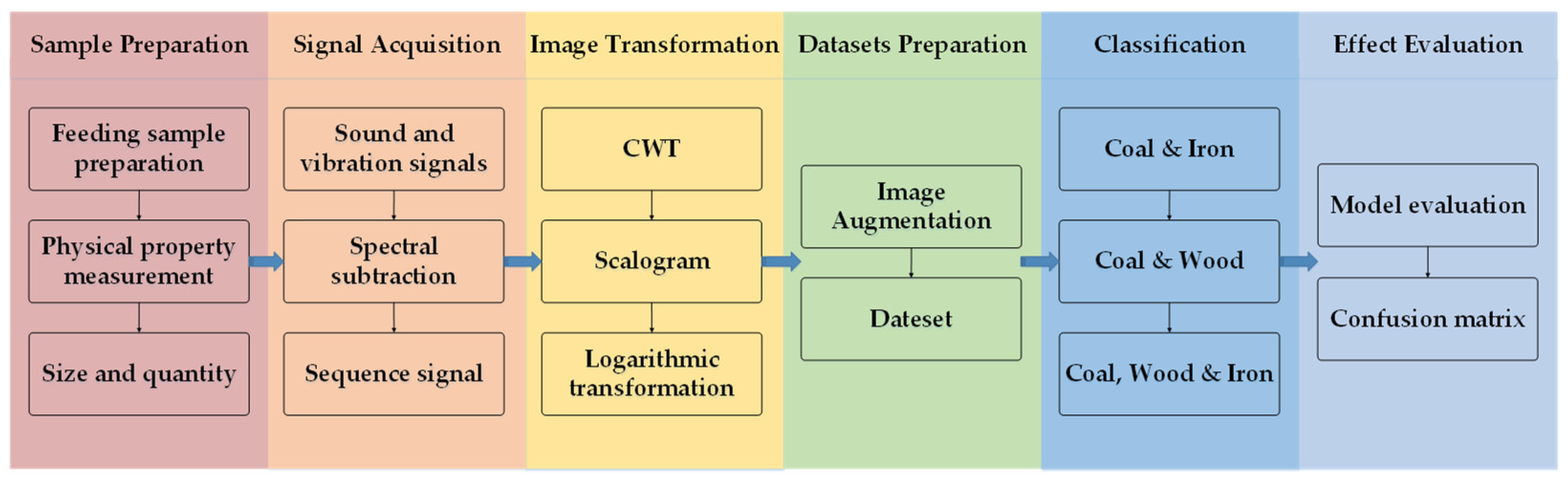
2. Methods
2.1. Feature Selection
- (1)
- Significant difference. The typical features of the different feeding materials should have a significant difference, which contributes to improving the classification effectiveness and greatly reducing the calculation amount.
- (2)
- Easy availability. Both data acquisition and analysis algorithms should be simple and easy to obtain, which allows rapid response to fault signals.
- (3)
- Broad applicability. The algorithm proposed in this paper aims to be applicable to not only different types but also different working conditions of two-tooth roll crushers. Broad applicability is the focus in the field of crusher fault diagnosis.
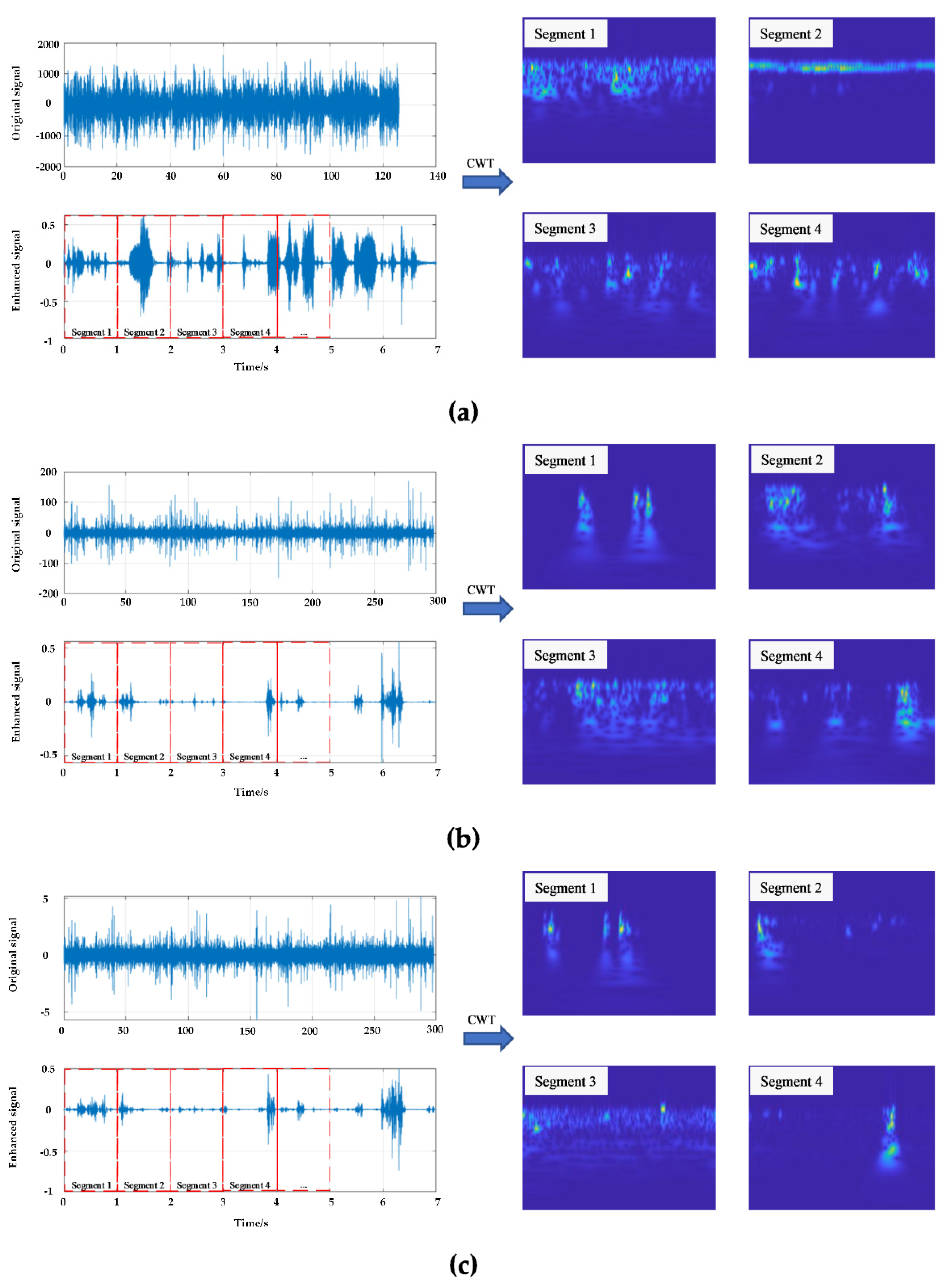
2.2. Spectral Subtraction
2.3. Continuous Wavelet Transforms
2.4. Deep Learning and Convolutional Neural Networks
2.5. Residual Neural Network
2.6. Data Augmentation
3. Study Case
3.1. Experimental Settings
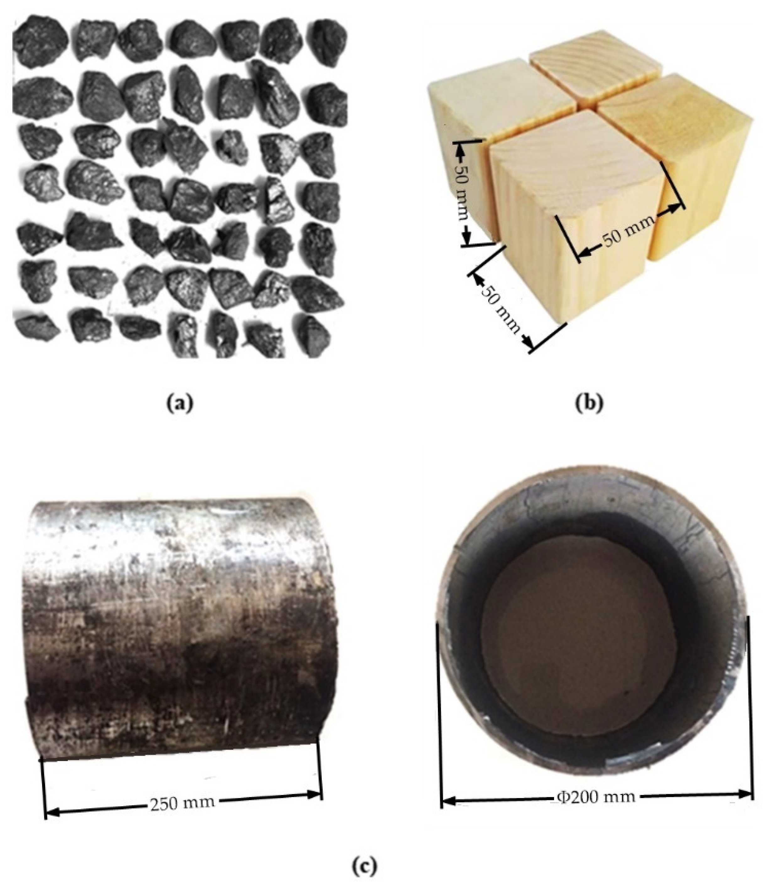
3.1.1. Sample Preparation
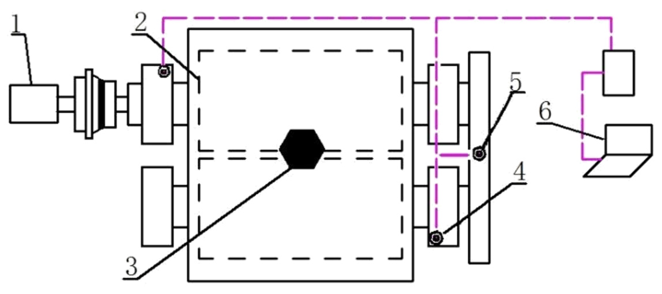
3.1.2. Test Device and Data Acquisition
3.1.3. Image Transformation
3.1.4. Dataset Preparation
3.2. Model Development
3.2.1. Model Building
3.2.2. Implementation Setting Details
3.3. Result Analysis
3.3.1. Model Evaluation
3.3.2. Confusion Matrix
4. Conclusions
- (1)
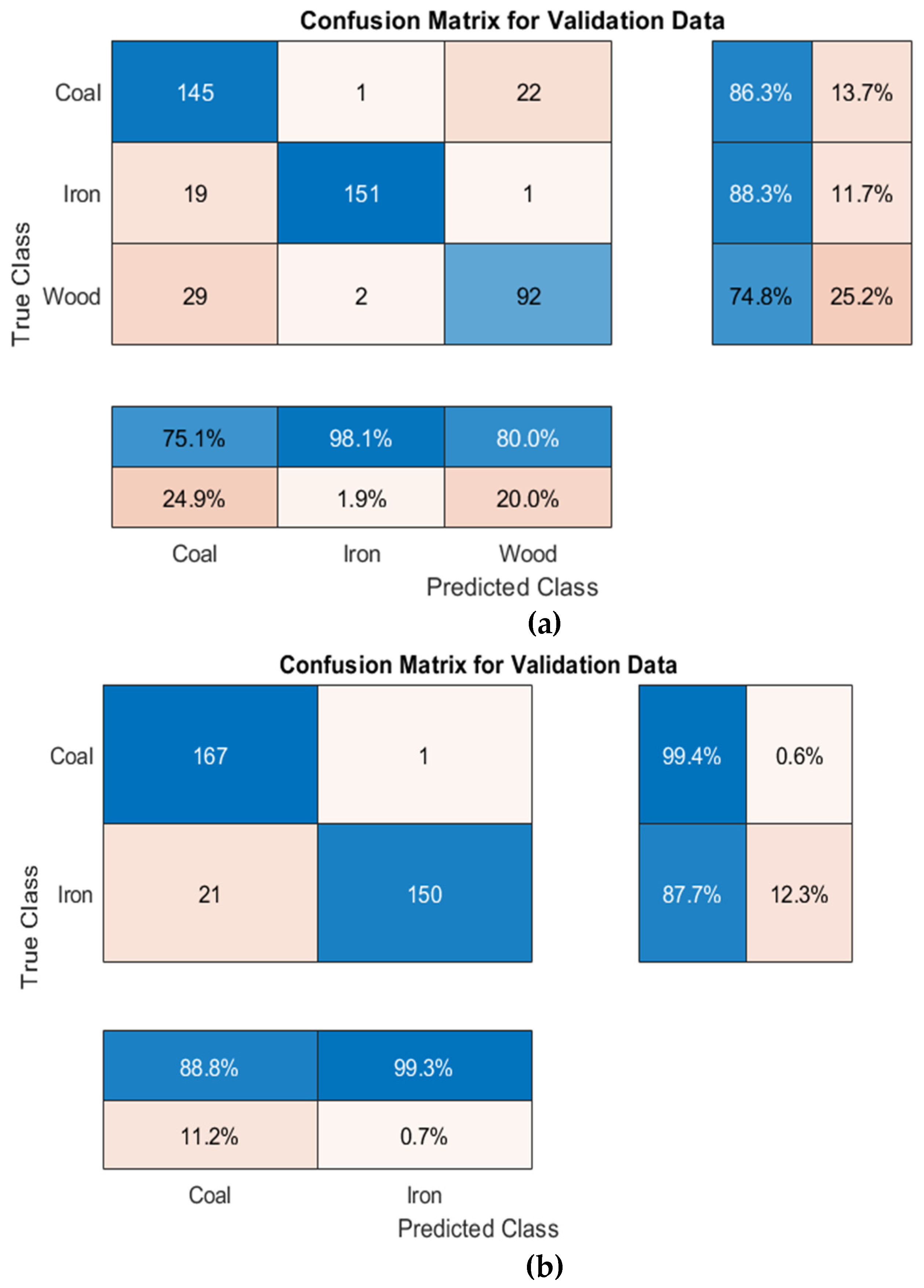
- Referring to Resnet-50, the image classification model based on deep learning established in this experiment has good classification performance for typical crushing equipment feeding materials of. However, when wood was present in the classification object, the similarity between coal and wood led to a decrease in accuracy. The accuracies of coal–iron–wood classification, coal–iron classification and coal–wood classification obtained in this paper were 84.0%, 93.5% and 80.1%, respectively.
- (2)
- A comparative analysis of the three classification cases revealed that iron had higher precision, sensitivity, specificity, and F1-Score in the confusion matrix, indicating that the feeding characteristics of iron were more obvious than those of the other materials. In addition, coal–wood classification accuracy was lower, considering that due to their having similar mechanical properties and physical characteristics, and the fact that both are more likely to be crushed and generate large amounts of energy at the moment of crushing, these characteristics cannot be easily distinguished by a single indicator alone. The reason that this affects the accuracy of the three classifications lies in the fact that coal and wood cannot be easily separated.
- (3)
- To improve the accuracy of coal–wood classification, in-depth research based on increasing the number of feature indicators and the volume of data is needed in the future. Considering production demand, the accuracy of the current classification model is able to fully satisfy the purpose of excluding harmful iron from the crushing chamber and provide technical core support for the design of a system for crusher operating status monitoring and fault diagnosis. In the future, deep learning can be further combined with mineral engineering to try to explore the problems of mineral processing and machinery from a new perspective.
Author Contributions
Funding
Conflicts of Interest
References
- Pan, Y. Development of China’s coal crushing equipment over the past 70 years and perspective. Coal Prep. Technol. 2019, 272, 32–36, 42. [Google Scholar] [CrossRef]
- Lieberwirth, H.; Hillmann, P.; Hesse, M. Dynamics in double roll crushers. Miner. Eng. 2017, 103, 60–66. [Google Scholar] [CrossRef]
- Zak, G.; Wylomanska, A.; Zimroz, R. Alpha-Stable Distribution Based Methods In The Analysis of The Crusher Vibration Signals For Fault Detection. Ifac Pap. 2017, 50, 4696–4701. [Google Scholar] [CrossRef]
- Jha, P.K.; Rajora, R. Fault Diagnosis of Coal Ring Crusher in Thermal Power Plant: A Case Study. In Proceedings of the 2016 International Conference on Automatic Control and Dynamic Optimization Techniques (ICACDOT), Pune, India, 9–10 September 2016; pp. 355–360. [Google Scholar]
- Liu, Q.; Song, B.; Ding, X.; Qin, S.J. Fault diagnosis of dynamic processes with reconstruction and magnitude profile estimation for an industrial application. Control Eng. Pract. 2022, 121, 105008. [Google Scholar] [CrossRef]
- Obuchowski, J.; Zimroz, R.; Wylomanska, A. Identification of cyclic components in presence of non-Gaussian noise–Application to crusher bearings damage detection. J. Vibroeng. 2015, 17, 1242–1252. [Google Scholar]
- Wylomanska, A.; Zimroz, R.; Janczura, J. Identification and stochastic modelling of sources in copper ore crusher vibrations. J. Phys. Conf. Ser. 2015, 628, 012125. [Google Scholar] [CrossRef] [Green Version]
- Rahimdel, M.J.; Karamoozian, M. Fuzzy TOPSIS method to primary crusher selection for Golegohar Iron Mine (Iran). J. Cent. South Univ. 2014, 21, 4352–4359. [Google Scholar] [CrossRef]
- Moshgbar, M.; Parkin, R.; Bearman, R.A. Application of fuzzy logic and neural network technologies in cone crusher control. Miner. Eng. 1995, 8, 41–50. [Google Scholar] [CrossRef]
- Asbjörnsson, G.; Erdem, I.; Evertsson, M. Application of the Hilbert transform for diagnostic and control in crushing. Miner. Eng. 2020, 147, 106086. [Google Scholar] [CrossRef]
- Wylomanska, A.; Zimroz, R.; Janczura, J.; Obuchowski, J. Impulsive Noise Cancellation Method for Copper Ore Crusher Vibration Signals Enhancement. IEEE Trans. Ind. Electron. 2016, 63, 5612–5621. [Google Scholar] [CrossRef]
- Laha, S.K.; Swarnakar, B.; Kansabanik, S.; Uke, K.J. Rub-Impact Fault Diagnosis of a Coal Crusher Machine by Using Ensemble Patch Transformation and Empirical Mode Decomposition. In Nonstationary Systems: Theory and Applications; Springer: Cham, Switzerland, 2022; pp. 265–278. [Google Scholar]
- Sun, Y.H.; Li, C.; Huang, M.F.; Jing, H. Garbage Crusher Fault Diagnosis Based on RBF Neural Network. Appl. Mech. Mater. 2009, 16, 971–975. [Google Scholar] [CrossRef]
- Li, X.; Li, C.; Huang, M.; Jing, H. The Fault Diagnosis of Garbage Crusher Based on Ant Colony Algorithm and Neural Network. In Proceedings of the 2009 Third International Conference on Genetic and Evolutionary Computing, Guilin, China, 14–17 October 2009; pp. 515–519. [Google Scholar]
- Ma, L.C.; Zhang, Y.; Lv, P.; Ca, F.; Liu, Y.H. Research on Fault Diagnosis System of Crusher Based on BP Neural Network. In Proceedings of the 2020 Chinese Control And Decision Conference (CCDC), Hefei, China, 22–24 August 2020; pp. 677–682. [Google Scholar]
- Olivier-Maget, N.; Negny, S.; Hetreux, G.; Le Lann, J.M. Fault diagnosis and process monitoring through model-based and case based reasoning. Comput-Aided Chem. Eng. 2009, 26, 345–350. [Google Scholar]
- Park, S.; Jung, D.; Nguyen, H.; Choi, Y. Diagnosis of Problems in Truck Ore Transport Operations in Underground Mines Using Various Machine Learning Models and Data Collected by Internet of Things Systems. Minerals 2021, 11, 1128. [Google Scholar] [CrossRef]
- Li, H.; Asbjörnsson, G.; Lindqvist, M. Image Process of Rock Size Distribution Using DexiNed-Based Neural Network. Minerals 2021, 11, 736. [Google Scholar] [CrossRef]
- Jia, L.; Yang, M.; Meng, F.; He, M.; Liu, H. Mineral Photos Recognition Based on Feature Fusion and Online Hard Sample Mining. Minerals 2021, 11, 1354. [Google Scholar] [CrossRef]
- Iwaszenko, S.; Róg, L. Application of Deep Learning in Petrographic Coal Images Segmentation. Minerals 2021, 11, 1265. [Google Scholar] [CrossRef]
- Chow, B.; Reyes-Aldasoro, C. Automatic Gemstone Classification Using Computer Vision. Minerals 2021, 12, 60. [Google Scholar] [CrossRef]
- Pan, Y.; Li, Z.; Zhu, C.; Liu, W.; Lang, J.; Wei, Y.; Yao, F.; Liu, Z. Research on the fault diagnosis of coal preparation equipment based on Artificial Neural Networks. In Proceedings of the XIX International Coal Preparation Congress, New Delhi, India, 13 November 2019. [Google Scholar]
- Chen, X. Research on Fault Identification System of Crusher Based on Signal Analysis and Convolution Neural Network. Master’s Thesis, China University of Mining & Technology, Beijing, China, 2021. [Google Scholar]
- Yan, Y. Research on Breaker Fault Identification Technology Based on Audio Signal Analysis. Master’s Thesis, China University of Mining & Technology, Beijing, China, 2020. [Google Scholar]
- Boll, S. Suppression of acoustic noise in speech using spectral subtraction. IEEE Trans. Acoust. Speech Signal Process. 1979, 27, 113–120. [Google Scholar] [CrossRef] [Green Version]
- Hao, L.; Cao, S.; Zhou, P.; Chen, L.; Zhang, Y.; Li, K.; Xie, D.; Geng, Y.; Cavaleri, L. Denoising Method Based on Spectral Subtraction in Time-Frequency Domain. Adv. Civ. Eng. 2021, 2021, 1–12. [Google Scholar] [CrossRef]
- Berouti, M.; Schwartz, R.; Makhoul, J. Enhancement of speech corrupted by acoustic noise. In Proceedings of the Acoustics, Speech, and Signal Processing, IEEE International Conference on ICASSP ’79, Washington, DC, USA, 2–4 April 1979. [Google Scholar]
- Ozawa, K.; Morise, M.; Sakamoto, S.; Watanabe, K. Sound Source Separation by Spectral Subtraction Based on Instantaneous Estimation of Noise Spectrum. In Proceedings of the 2019 6th International Conference on Systems and Informatics (ICSAI), Shanghai, China, 2–4 November 2019; pp. 1137–1142. [Google Scholar]
- Yan, X.; Yang, Z.; Wang, T.; Guo, H. An Iterative Graph Spectral Subtraction Method for Speech Enhancement. Speech Commun. 2020, 123, 35–42. [Google Scholar] [CrossRef]
- Siam, A.I.; El-khobby, H.A.; Elnaby, M.M.A.; Abdelkader, H.S.; El-Samie, F.E.A. A Novel Speech Enhancement Method Using Fourier Series Decomposition and Spectral Subtraction for Robust Speaker Identification. Wirel. Pers. Commun. 2019, 108, 1055–1068. [Google Scholar] [CrossRef]
- Zhang, Q.-y.; Li, G.-l.; Huang, Y.-b. An efficient retrieval approach for encrypted speech based on biological hashing and spectral subtraction. Multimed. Tools Appl. 2020, 79, 29775–29798. [Google Scholar] [CrossRef]
- Stark, H.-G. Continuous wavelet transform and continuous multiscale analysis. J. Math. Anal. Appl. 1992, 169, 179–196. [Google Scholar] [CrossRef] [Green Version]
- Shi, Y.; Ruan, Q. Continuous wavelet transforms. In Proceedings of the 7th International Conference on Signal Processing, ICSP ’04, Beijing, China, 31 August–4 September 2004; Volume 201, pp. 207–210. [Google Scholar]
- Yuan, L.; Lian, D.; Kang, X.; Chen, Y.; Zhai, K. Rolling Bearing Fault Diagnosis Based on Convolutional Neural Network and Support Vector Machine. IEEE Access 2020, 8, 137395–137406. [Google Scholar] [CrossRef]
- Rioul, O.; Vetterli, M. Wavelets and signal processing. IEEE Signal Process. Mag. 1991, 8, 14–38. [Google Scholar] [CrossRef] [Green Version]
- LeCun, Y.; Bengio, Y.; Hinton, G. Deep learning. Nature 2015, 521, 436–444. [Google Scholar] [CrossRef] [PubMed]
- Deng, J.; Guo, J.; Xue, N.; Zafeiriou, S. ArcFace: Additive Angular Margin Loss for Deep Face Recognition. In Proceedings of the 2019 IEEE/CVF Conference on Computer Vision and Pattern Recognition (CVPR), Long Beach, CA, USA, 15–20 June 2019; pp. 4685–4694. [Google Scholar]
- Daugman, J. How Iris Recognition Works. IEEE Trans. Circuits Syst. Video Technol. 2004, 14, 21–30. [Google Scholar] [CrossRef]
- Chang, S.L.; Chen, L.S.; Chung, Y.C.; Chen, S.W. Automatic License Plate Recognition. IEEE Trans. Intell. Transp. Syst. 2004, 5, 42–53. [Google Scholar] [CrossRef]
- Wen, Z.; Zhou, C.; Pan, J.; Nie, T.; Jia, R.; Yang, F. Froth image feature engineering-based prediction method for concentrate ash content of coal flotation. Miner. Eng. 2021, 170, 107023. [Google Scholar] [CrossRef]
- Liu, Y.; Zhang, Z.; Liu, X.; Wang, L.; Xia, X. Performance evaluation of a deep learning based wet coal image classification. Miner. Eng. 2021, 171, 107126. [Google Scholar] [CrossRef]
- Ioffe, S.; Szegedy, C. Batch Normalization: Accelerating Deep Network Training by Reducing Internal Covariate Shift. In Proceedings of the 32nd International Conference on International Conference on Machine Learning, Lille, France, 6–11 July 2015; pp. 448–456. [Google Scholar]
- Salman, K.; Hossein, R.; Syed Afaq Ali, S.; Mohammed, B.; Gerard, M.; Sven, D. A Guide to Convolutional Neural Networks for Computer Vision; Morgan & Claypool: San Rafael, CA, USA, 2018; p. 1. [Google Scholar]
- Jarrett, K.; Kavukcuoglu, K.; Ranzato, M.; LeCun, Y. What is the best multi-stage architecture for object recognition? In Proceedings of the 2009 IEEE 12th International Conference on Computer Vision, Kyoto, Japan, 29 September–2 October 2009; pp. 2146–2153. [Google Scholar]
- He, K.; Zhang, X.; Ren, S.; Sun, J. Deep Residual Learning for Image Recognition. In Proceedings of the 2016 IEEE Conference on Computer Vision and Pattern Recognition (CVPR), Las Vegas, NV, USA, 27–30 June 2016. [Google Scholar]
- He, K.; Zhang, X.; Ren, S.; Sun, J. Delving Deep into Rectifiers: Surpassing Human-Level Performance on ImageNet Classification. In Proceedings of the CVPR, Boston, MA, USA, 7–12 June 2015. [Google Scholar]
- Wu, Z.; Shen, C.; Hengel, A. Wider or Deeper: Revisiting the ResNet Model for Visual Recognition. Pattern Recognit. 2019, 90, 119–133. [Google Scholar] [CrossRef] [Green Version]
- Ma, L.; Shuai, R.; Ran, X.; Liu, W.; Ye, C. Combining DC-GAN with ResNet for blood cell image classification. Med. Biol. Eng. Comput. 2020, 58, 1251–1264. [Google Scholar] [CrossRef] [PubMed]
- Razavi, M.; Alikhani, H.; Janfaza, V.; Sadeghi, B.; Alikhani, E. An Automatic System to Monitor the Physical Distance and Face Mask Wearing of Construction Workers in COVID-19 Pandemic. SN Comput. Sci. 2022, 3, 27. [Google Scholar] [CrossRef] [PubMed]
- Zhao, M.; Zhong, S.; Fu, X.; Tang, B.; Pecht, M. Deep Residual Shrinkage Networks for Fault Diagnosis. IEEE Trans. Ind. Inform. 2020, 16, 4681–4690. [Google Scholar] [CrossRef]
- Shorten, C.; Khoshgoftaar, T.M. A survey on Image Data Augmentation for Deep Learning. J. Big Data 2019, 6, 60–108. [Google Scholar] [CrossRef]
- Zhou, C.; Pan, Y.; Lu, M. ZKB shear breaker and analysis on its performance. Coal Prep. Technol. 2004, 6, 21–23. [Google Scholar]
- Olhede, S.C.; Walden, A.T. Generalized Morse wavelets. IEEE Trans. Signal Process. 2002, 50, 2661–2670. [Google Scholar] [CrossRef] [Green Version]
- Lilly, J.M.; Olhede, S.C. Generalized Morse Wavelets as a Superfamily of Analytic Wavelets. IEEE Trans. Signal Process. 2012, 60, 6036–6041. [Google Scholar] [CrossRef] [Green Version]
- Charles, E.M. Basic principles of ROC analysis. Semin. Nucl. Med. 1978, 8, 283–298. [Google Scholar] [CrossRef]
- Fawcett, T. An introduction to ROC analysis. Pattern Recognit. Lett. 2006, 27, 861–874. [Google Scholar] [CrossRef]


| Articles | Signal Type | Selected Features | Classification Algorithm |
|---|---|---|---|
| Pan et al. [22] | AS | Amplitude at a frequency of 360 Hz in the power spectrum | BP neural network |
| Amplitude wave peak in the middle frequency band | |||
| Standard deviation of logarithmic amplitude in high frequency | |||
| Chen et al. [23] | SPS | Short-term energy | Linear superposition |
| Short-time magnitude | |||
| Power spectrum | |||
| Yan et al. [24] | AS | Signal gray-scale | LeNet-5 |
| Time-frequency diagram of the short-time Fourier transform | |||
| Time-frequency diagram of continuous Wavelet Transform | |||
| (AS—Audio Signals, SPS—Sound Pressure Signals) | |||
| Sample | Taixi Coal | Pine | Q235B |
|---|---|---|---|
| Quantity | 500 | 500 | 1 |
| Size/mm | 45~55 | 50 × 50 × 50 | Φ 200 × 250 × 10 |
| Density/g·cm−3 | 1.450 | 0.519 | 7.830 |
| Tensile Strength/MPa | 0. 953 | 102.8 (parallel to grain) | 375~500 |
| Elastic Modulus/MPa | 3.40 | 16.30 (x) | 210 |
| 0.57 (y) | |||
| 1.10 (z) | |||
| Poisson Ratio | 0.201 | 0.570 (xy) | 0.274 |
| 0.310 (yz) | |||
| 0.420 (xz) |
| Data Size | Mean Validation Accuracy | Standard Deviation |
|---|---|---|
| 100 | 73.89% | 2.6411 |
| 200 | 81.28% | 2.1089 |
| 300 | 83.00% | 1.4856 |
| 400 | 82.56% | 0.8589 |
| 500 | 84.24% | 0.5925 |
| 600 | 81.19% | 0.9979 |
| Technical Parameters | Value |
|---|---|
| Feed Size/mm | 300 × 200 × 3 |
| Product Particle Size/mm | 20 × 20 |
| Boundary Dimension/mm | 1366 × 466 × 485 |
| Operating Weight/kg | 320 |
| Maximum Current/a | 6.8 |
| Power/kw | 3 |
| Supply Voltage/v | 380 |
| Input Speed/r·min−1 | 1420 |
| Model | Input | Pooling Layer Active Function | Fully Connected Layer Active Function | Parameter | FLOPs |
|---|---|---|---|---|---|
| 224 × 224 | ReLU | sigmoid | 25.5 × 10⁶ | 4.1 × 10⁹ |
| Parameter Name | Selected Value | |
|---|---|---|
| Optimization | Optimization name | SGDM |
| Learning rate | 1 × 10⁻³ | |
| Momentum | 0.9 | |
| Loss function | Cross entropy loss | |
| Fitting | Batch size | 32 |
| Epochs | 30 | |
| Environment | GPU | NVIDIA GeForce RTX 2060 |
| Platform | Python 3.8 |
| Feed Materials | Train Loss | SD | Train Accuracy | SD | Valid Loss | SD | Valid Accuracy | SD |
|---|---|---|---|---|---|---|---|---|
| Coal, Wood & Iron | 0.2271 | 0.0784 | 89.38% | 5.4486 | 0.5925 | 0.0476 | 84.24% | 0.6107 |
| Coal & Iron | 0.0002 | 0.0003 | 100% | 0 | 0.2262 | 0.0337 | 93.78% | 0.4464 |
| Coal & Wood | 0.2619 | 0.0816 | 84.69% | 5.1254 | 0.5380 | 0.0630 | 80.07% | 0.9597 |
| Materials | Accuracy | Precision | Sensitivity | Specificity | F1-Score |
|---|---|---|---|---|---|
| Coal-Iron-Wood | |||||
| Coal | 84.0% | 75.1% | 86.3% | 83.7% | 80.3% |
| Iron | 98.1% | 88.3% | 99.0% | 92.9% | |
| Wood | 80.0% | 74.8% | 93.2% | 77.3% | |
| Coal-Iron | |||||
| Coal | 93.5% | 88.8% | 99.4% | 87.7% | 93.8% |
| Iron | 99.3% | 87.7% | 99.4% | 93.1% | |
| Coal-Wood | |||||
| Coal | 80.1% | 81.3% | 85.1% | 73.2% | 83.2% |
| Wood | 78.3% | 73.2% | 85.1% | 75.7% | |
Publisher’s Note: MDPI stays neutral with regard to jurisdictional claims in published maps and institutional affiliations. |
© 2022 by the authors. Licensee MDPI, Basel, Switzerland. This article is an open access article distributed under the terms and conditions of the Creative Commons Attribution (CC BY) license (https://creativecommons.org/licenses/by/4.0/).
Share and Cite
Pan, Y.; Bi, Y.; Zhang, C.; Yu, C.; Li, Z.; Chen, X. Feeding Material Identification for a Crusher Based on Deep Learning for Status Monitoring and Fault Diagnosis. Minerals 2022, 12, 380. https://doi.org/10.3390/min12030380
Pan Y, Bi Y, Zhang C, Yu C, Li Z, Chen X. Feeding Material Identification for a Crusher Based on Deep Learning for Status Monitoring and Fault Diagnosis. Minerals. 2022; 12(3):380. https://doi.org/10.3390/min12030380
Chicago/Turabian StylePan, Yongtai, Yankun Bi, Chuan Zhang, Chao Yu, Zekui Li, and Xi Chen. 2022. "Feeding Material Identification for a Crusher Based on Deep Learning for Status Monitoring and Fault Diagnosis" Minerals 12, no. 3: 380. https://doi.org/10.3390/min12030380
APA StylePan, Y., Bi, Y., Zhang, C., Yu, C., Li, Z., & Chen, X. (2022). Feeding Material Identification for a Crusher Based on Deep Learning for Status Monitoring and Fault Diagnosis. Minerals, 12(3), 380. https://doi.org/10.3390/min12030380