Article

3D Inversion of Magnetic Gradient Tensor Data Based on Convolutional Neural Networks

1
Institute of Geophysics and Geomatics, China University of Geosciences, Wuhan 430074, China
2
School of Information and Communication, Guilin University of Electronic Technology, Guilin 541004, China
3
State Key Laboratory of Geological Processes and Mineral Resources, China University of Geosciences, Wuhan 430074, China
4
Badong National Observation and Research Station of Geohazards, China University of Geosciences, Wuhan 430074, China
5
Institute of Geological Survey, China University of Geosciences, Wuhan 430074, China
*
Author to whom correspondence should be addressed.
Minerals 2022, 12(5), 566; https://doi.org/10.3390/min12050566
Submission received: 31 March 2022 / Revised: 24 April 2022 / Accepted: 26 April 2022 / Published: 30 April 2022
(This article belongs to the Special Issue Electromagnetic Exploration: Theory, Methods and Applications)

Abstract

:
High-precision vector magnetic field detection has been widely used in the fields of celestial magnetic field detection, aeromagnetic detection, marine magnetic field detection and geomagnetic navigation. Due to the large amount of data, the 3D inversion of high-precision magnetic gradient vector data often involves a large number of computational requirements and is very time-consuming. In this paper, a 3D magnetic gradient tensor (MGT) inversion method is developed, based on using a convolutional neural network (CNN) to automatically predict physical parameters from the 2D images of MGT. The information of geometry, depth and parameters such as magnetic inclination (I), magnetic declination (D) and magnetization susceptibility of magnetic anomalies is extracted, and a 3D model is obtained by comprehensive analysis. The method first obtains sufficient MGT data samples by forward modeling of different magnetic anomalies. Then, we use an improved CNN with shear layers to achieve the prediction of each magnetic parameter. The reliability of the algorithm is verified by numerical simulations of synthetic models of multiple magnetic anomalies. MGT data of the Tallawang magnetite diorite deposit in Australia are also predicted by using this method to obtain a slab model that matches the known geological information. The effects of sample size and noise level on the prediction accuracy are discussed. Compared with single-component prediction, the results of multi-component joint prediction are more reliable. From the numerical model study and the field data validation, we demonstrate the capability of using CNNs for inversing MGT data.

1. Introduction

Tensor gradient measurement in magnetic exploration is an important detection method [1,2,3]. Full tensor measurement, which can not only retain the intensity and direction information of magnetic vectors but can also suppress the common-mode field from the core, the regional field from the deep crust and the geomagnetic variation from the ionosphere and magnetosphere. Magnetic gradient tensor (MGT) surveys can reflect detailed features with higher resolution, such as superimposed anomalous bodies [4,5]. With the advantages of strong anti-interference ability and high detection accuracy, they are widely used in the fields of celestial magnetic field detection, aeromagnetic investigation, ocean magnetic field exploration and geomagnetic navigation [6,7], and are currently the main method for ocean, aeromagnetic and celestial magnetic detection [8].
The inversion of magnetic data is critical for quantitative geological interpretation. Geometric information such as the horizontal position, depth and boundary of an anomaly source, as well as the quantitative information of physical parameters such as magnetization susceptibility, magnetic inclination and magnetic declination inside the anomaly, can be obtained by polyhedral dissection of the irregular anomaly followed by physical inversion [9,10]. MGT data were first used for military target detection, and MGT algorithms were developed for military use in isolated magnetic dipole target detection by Frahm [11,12]. Zhang et al. [13] extended the Eulerian inverse fold product method and applied it to the interpretation of gravity gradient tensor data, solving the MGT inversion problem for the case of multiple magnetic dipoles. Schmidt and Clark [2] further analyzed the correspondence between the eigenvalues of the magnetic tensor matrix and the distribution of the magnetic sources and extended the method to the interpretation of the multi-component phase-constrained MGT data method. Zhdanov et al. [14] proposed two-dimensional potential field migration and focused inversion [15], and later developed a potential field migration algorithm for gravity gradient measurements [16]. Cai and Zhdanov [17] used the principle of potential field migration to achieve multi-component inversion of gravitation and MGTs, and improved their inversion accuracy with a focused algorithm. Sun and Li [18] applied the method of clustered c-means to invert gravity and magnetic potential field data and obtained high-resolution inversion results, and extended their method to the joint inversion of gravity and magnetic law data. Zhdanov and Lin [19] proposed an adaptive multinary inversion approach for recovering sharp models. Liu and Hu [20] proposed an iterative algorithm for magnetization vector inversion (M-IDI) which iteratively calculated the magnetic dipole direction after recovering the magnetization direction from the magnetization intensity. Geng [21] used the edge probability statistics method to realize the 3D physical inversion of potential field data, which provided new ideas for potential field data inversion.
In recent years, deep learning techniques in the field of artificial intelligence have made many breakthroughs in image recognition and classification, natural language processing, etc. They have also been used for solving geophysical exploration problems. In the field of geophysics, machine learning algorithms have been increasingly used in seismic signal processing, data reconstruction and fault identification.
Raiche [22] proposed the early inversion of physical parameters by pattern recognition and neural network methods and developed an empirical paradigm. Spichak and Popova [23] used artificial neural network methods for the inversion of geomagnetic macro parameters. Sun and Li [24] proposed a multi-domain rock physical constraint inversion and the geological discretization method based on generalized fuzzy clustering algorithms, which strengthened the connection between rock properties and inversion results compared to traditional inversion methods. Singh and Sharma [25] used the fuzzy clustering method to identify different geological units from resistivity imaging results.
Puzyrev [26] used CNNs to invert the location and dimensions of subsurface anomalies from controlled-source electromagnetic data. Noh [27] implemented a CNN-based 3D inversion of frequency-domain airborne EM data, and the results showed that the CNN still maintained high resolution when the amount of synthetic data was small. Liu [28] proposed a DC resistivity fully connected network (FCN) inversion method based on smoothing constraints and depth weighting, which effectively improved the accuracy of the solution. Using a Unet CNN, Yang et al. [29] inverted 3D gravity data and verified that CNNs can be used for geophysical gravity data processing. Nurindrawati and Sun [30] extracted magnetic direction parameters (magnetic inclination (I) and magnetic declination (D)) for magnetic total field data using a dual CNN structure classification recognition method to improve the automatic recognition efficiency of magnetic direction parameters; this method’s classification recognition was more suitable for the extraction of specific sensitive information. Li [31] proposed a sample generation algorithm of simplifying and then purifying features in cases with a lack of effective samples for geomagnetic neural network inversion which could effectively reduce the number of original samples and improve the sample generation efficiency. Hu and Liu [32] implemented 3D magnetic total field inversion using an FCN and deep neural network (DNN) in deep learning; taking the magnetic total field data of the Galinge iron ore deposit in China as an example, the magnetization distribution of the hidden iron ore body based on their neural network’s inversion matched well with drilling detection results, which further verified the feasibility and reliability of the method. Using the Linet-5 CNN architecture, He and Cai [33] proposed a method for depth-to-basement inversion directly from gravity data which improved the automation of converting gravity anomalies to basin depth.
Neural networks have achieved some success in geophysical inversion, but are less often used in magnetic field tensor gradient inversion. An airborne MGT survey involves a large amount of data acquisition, which requires a large amount of computationally intensive processes such as magnetic vector data processing and 3D inversion. Furthermore, CNNs have achieved excellent real-world results in image recognition, and the image samples of MGT components provide a theoretical basis for the CNN image recognition method; thus, we introduce a CNN into our MGT inversion approach. We validate the feasibility and accuracy of the algorithm via two synthetic simulation models and a case study featuring actual measurements of the Tallawang magnetite sillimanite deposit in Australia.
This paper is structured as follows. First, the method background and basic theoretical approach are introduced in Section 2. This contains the principle of MGT forward modeling and inversion, and the principles and process of CNN image recognition, then briefly introduces the adopted AlexNet network [34] and our improvements. The third section of the numerical model implementation discusses the generation of synthetic model samples, the construction and optimization of the CNN, the identification of magnetic parameters and the statistics of the prediction fitness of the two comprehensive simulation models for single and double blocks. The effects of the optimization of CNN parameters, sample noise and number of factors on the model’s recognition accuracy are discussed. The tensor gradient components and the total field are also analyzed for the comparison of the recognition accuracy of the physical parameters. Section 4 presents a case study of an example model of the Tallawang magnetite diorite mine in Australia. Finally, Section 5 provides a brief summary of the application of neural networks in MGT inversion.

2. Methodology

2.1. Forward Modeling

This study is based on using the construction of MGT forward modeling to generate a large number of sample images; thus, it is necessary to analyze the physical meaning of the potential field data and the forwarding and inversion equations.
The target of magnetic exploration is the subsurface magnetic inhomogeneous body, and the measurement objects are the magnetic induction intensity and spatial variation rate. Note that the magnetic field intensity mentioned in magnetic exploration refers to the magnetic induction intensity. The magnetic field vector is defined as B , then its components in three orthogonal directions are described as B x , B y and B z and the derivatives of each axial component in the x, y and z directions can be obtained as magnetic tensor components: B i j , i , j = x , y , z . For an arbitrary 3D anomaly, the magnetic field B is calculated per [35,36,37,38] as:
B ( r ) = C m r 0 Φ ( r ) = C m r 0 V M ( r 0 ) r 0 1 | r r 0 | d v ,  
where C m = 10 7 H e n r y / m is the magnetization constant, Φ is the magnetic scalar potential, r is the position vector of observation, r 0 is the position vector of integration, v is the volume element and the magnetization intensity vector is M .
The components of the magnetic field, in three orthogonal directions, are defined as:
B x = μ 0 4 π { M x v 2 ( x ξ ) 2 ( y η ) 2 ( z ζ ) 2 r 5 d v + M y v 3 ( x ξ ) ( y η ) r 5 d v + M z v 3 ( x ξ ) ( z ζ ) r 5 d v }
B y = μ 0 4 π { M x v 3 ( x ξ ) ( y η ) r 5 d v + M z v 3 ( y η ) ( z ζ ) r 5 d v + M y v 2 ( y η ) 2 ( x ξ ) 2 ( z ζ ) 2 r 5 d v }
B z = μ 0 4 π { M x v 3 ( x ξ ) ( z ζ ) r 5 d v + M y v 3 ( y η ) ( z ζ ) r 5 d v + M z v 2 ( z ζ ) 2 ( x ξ ) 2 ( y η ) 2 r 5 d v }
where (ξ, η and ζ) are the coordinates within the magnetic anomaly and (x, y and z) are the observed coordinates.
Then, from the derivatives of Equations (2)–(4), respectively, the MGT matrix G can be obtained as follows [39]:
G = [ B x x B x y B x z B y x B y y B y z B z x B z y B z z ] = [ B x x B x y B x z B y x B y y B y z B z x B z y B z z ]
The above, Equation (5), contains the equations of the MGT forward modeling theory.

2.2. CNN

A CNN is a special feed-forward neural network inspired by the neural mechanisms of animal vision [34,40]. A typical CNN network structure consists of an input layer, a series of convolutional layers, a nonlinear activation layer, a pooling layer, a fully connected layer and an output layer. Hinton has previously set the number of network layers of a CNN to nine in order to alleviate the local optimal solution [41]. These multilayered network structures, which we call deep learning network structures [42], include residual neural networks (ResNets), long short-term memory networks (LSTMs), generative adversarial networks (GANs), etc. The CNN-based classification recognition framework used in this study is shown in Figure 1.
The most unique feature of CNNs is that each contains a convolutional layer. During the learning process of the convolutional layer, a CNN learns the local information of each image by sharing the weights of multiple convolutional kernels (or feature detectors), which are used to construct an abstract feature map. This convolutional kernel-sharing feature greatly reduces the number of parameters required to train the network. Since trained detectors can be repeatedly used to detect abstract features in images combinatorially through convolutional layers, CNNs require relatively fewer parameters compared to other neural network structures, making them more suitable for complex image recognition tasks. They have been widely used in the fields of image classification, target body localization, etc.
Neural networks can fit properties of linear or nonlinear physical variation by adjusting the weight coefficients of each neuron in their hidden layer, and therefore can also fit the partial differential equation (PDE)-solving process to achieve faster PDE solutions [43,44]. It has been shown that shallow networks can be viewed as operators; extending this theory to deep neural networks, the neural network model DeepONet( V0.11.2, Division of Applied Mathematics, Brown University, Providence, RI 02912, USA ) [45], which approximates linear and nonlinear operators, was proposed. The MGT inversion problem is a process of solving partial differential equations (PDEs) in reverse and a neural network can quickly solve PDEs, providing a theoretical basis for fast MGT inversion.
The main goal of this research is to predict each physical parameter and geometry of a magnetic source based on its MGT measurements using machine learning and, in particular, deep CNNs. To this end, we utilize independent prediction models for each parameter prediction; in other words, the prediction order mechanism can be adjusted to meet the needs of sensitive-parameter prediction, either distributed or independently identified in parallel. This prediction mechanism has higher effectiveness, accuracy and applicability. In other words, when a certain parameter of the magnetic source is of interest, the prediction of other detailed parameters is attempted, thus saving energy compared the overall predictions and measurements, especially when the detection result is not the target body sought. In addition, single-parameter prediction, a single lightweight prediction approach, is less computationally intensive and faster in training and prediction compared to overall prediction.
To verify the feasibility of the algorithm, the relatively lightweight CNN architecture AlexNet (University of Toronto, CAN) [34] is chosen for this study and an optimized AlexNet network is applied to parameter prediction in this study, as shown in Figure 2. Compared with other CNN models, this network structure has fewer layers to ensure certain prediction accuracy, which reduces the amount of operations and is suitable for the test platform of this study. The software testing environment is: Python (V3.5) + TensorFlow-GPU (V2.1.0) + Keras (V2.2.4), and the testing hardware is: HP Z8G4/ Intel Gold6148x2/ 512GBDDR4/Nvidia 208Ti x2 (Ubuntu 20.04LTS, HP, Palo Alto, CA, USA).
AlexNet uses ReLU as the activation function of its CNN [46], solves the gradient dispersion problem of Sigmoid when the network is deeper [47], uses Adam optimizer [48] and increases the training speed, but in practical tests we change the activation function to a combination of ELU and LeakyReLU [49,50], obtaining better convergence. A Dropout regularization mechanism is invoked during training to avoid model overfitting [51], and in the real test we introduce two Dropout layers, both with a shear rate of 20%. In addition, AlexNet includes a layer re-use network (LRN) layer that creates a competition mechanism for the activity of local neurons, boosting the neurons in which the response is relatively large and suppressing other neurons with smaller feedback, enhancing the generalization ability of the model.
In the actual test, the original AlexNet network architecture has low prediction accuracy and slow convergence speed. As such, we improve the original model as needed, as follows.
(a) The original image sample is 560 × 420 pixels, first normalized to 420 × 420 pixels. The amount of information around the graph is small. In order to reduce the amount of operations, the periphery is cropped by 10 pixels to 400 × 400 pixels and then compressed to 200 × 200 pixels for use as training samples. (b) The number of convolution kernels in the first convolution layer is 512. The size of the convolutional kernel is 1 × 1, which is beneficial for improving the extraction of weak information from the original sample. (c) In the process of actual testing, the activation function can be ELU, LeackRLU or a combination of both, which is beneficial for increasing the convergence speed. (d) Two additional layers of shearing are added and the shearing rate reaches 20%, which is beneficial for improving the generalization ability. (e) The learning rate is 10 × 10−6, which can prevent model oscillation by reducing the learning rate [52]. (f) The Miner Batch Size is set to 32. The smaller the value, the further improvement in convergence [53].
Of course, there are many optimization methods [54], but we implement only the improvements listed above to verify the feasibility of the scheme; nonetheless, its prediction and verification accuracy can reach more than 90% after 200 Epochs in the real test, which satisfies the prediction accuracy requirement.

2.3. The Overall Research Framework

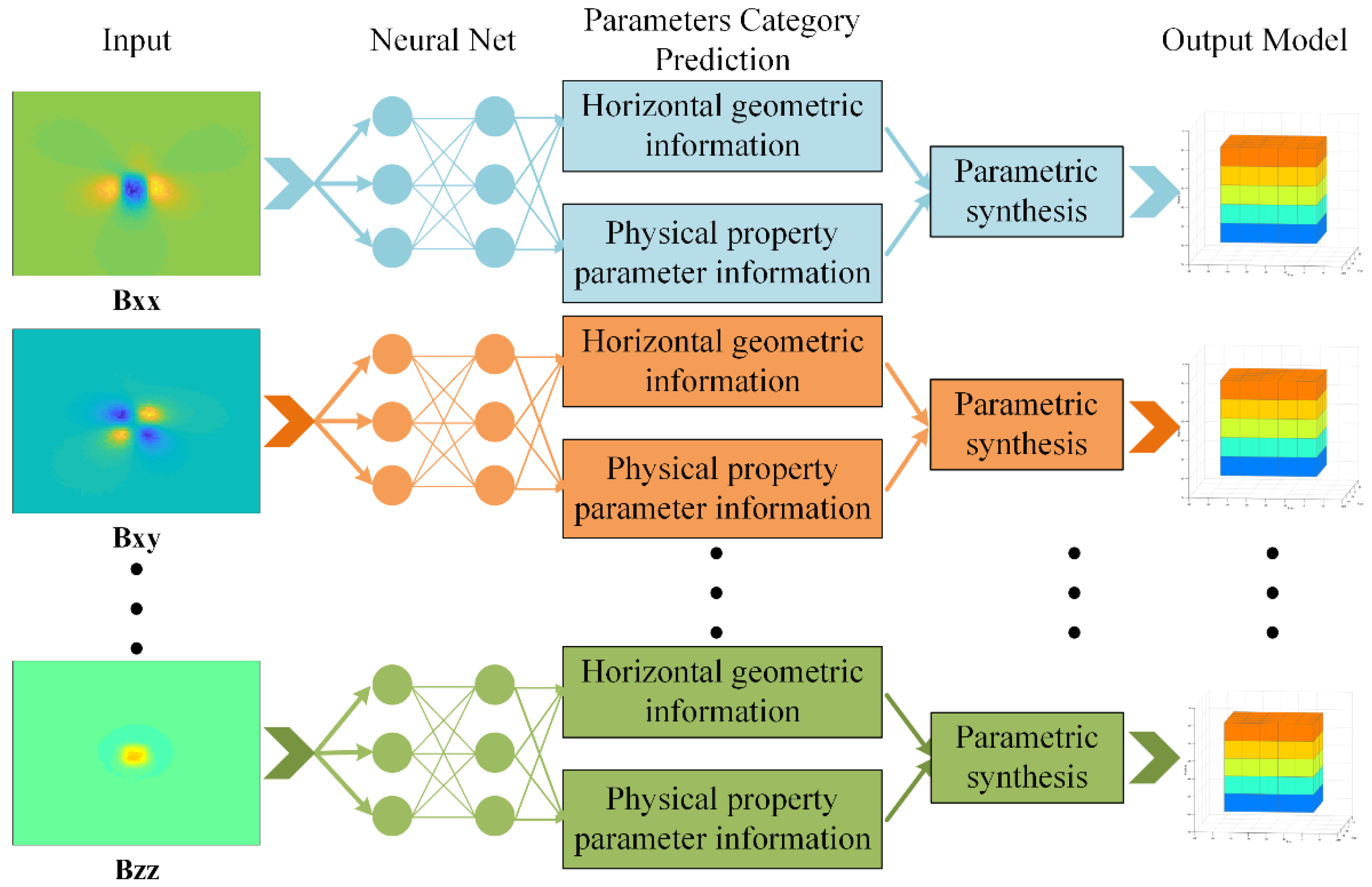
The overall research structure of this study is shown in Figure 3, with 2D images of each independent component of the MGT: B x x , B x y , B x z , B y y , B y z and B z z . The 2D images here are the images of the horizontal plane on the X and Y axis. The component images are obtained either from the synthetic input model forward modeling or real measurement acquisition. Each component’s image is predicted by the trained deep CNN with horizontal geometric information and magnetic parameter information. To further obtain the inversion results, we also need to synthesize all the predicted results with parameters and generate a new model directly into a map, which is the inversion result we are looking for. In general, we first judge the horizontal position; in other words, we first judge whether there is an anomaly in the detection area. Secondly, we judge the geometry of the anomaly; that is, we identify the type of target body. If the detected target body matches the type of target body we are looking for, then we can predict its depth information and more detailed magnetic parameters (magnetization susceptibility, magnetic inclination (I), magnetic declination (D), etc.). Assuming that the object to be found is a specific target body and, in addition, that the targeted body and boundary identification methods (based on the potential field) are well established [7,55,56,57,58], we assume that the shape characteristics of each magnetic anomaly are well-known
The prediction process is shown in Figure 4. The inversion in this research work differs from other machine learning inversions in that we do not use the profile images of depth and horizontal axes as training samples for inversion, but directly use horizontal 2D images, which are consistent with the actual detection results projected onto maps. In addition, instead of direct inversion, the geometric information, depth and physical parameters of the target body are predicted first, and then the 3D inversion model is derived by parameter synthesis after the required information is predicted. The MGT contains several independent components, each of which can be used to extract and invert the physical parameters, and if the inversion results of each independent component are combined, the joint inversion of multiple components can be realized.

3. Method

3.1. Forward Model

Seven models are tested in this study, as shown in Table 1 below. These types include spherical, single-block, double-block, three-block and four-block. For this work, we assume predictions for a specific target body; i.e., only the models in the model library are probed, and for this purpose the size of the target body is assumed to be known.
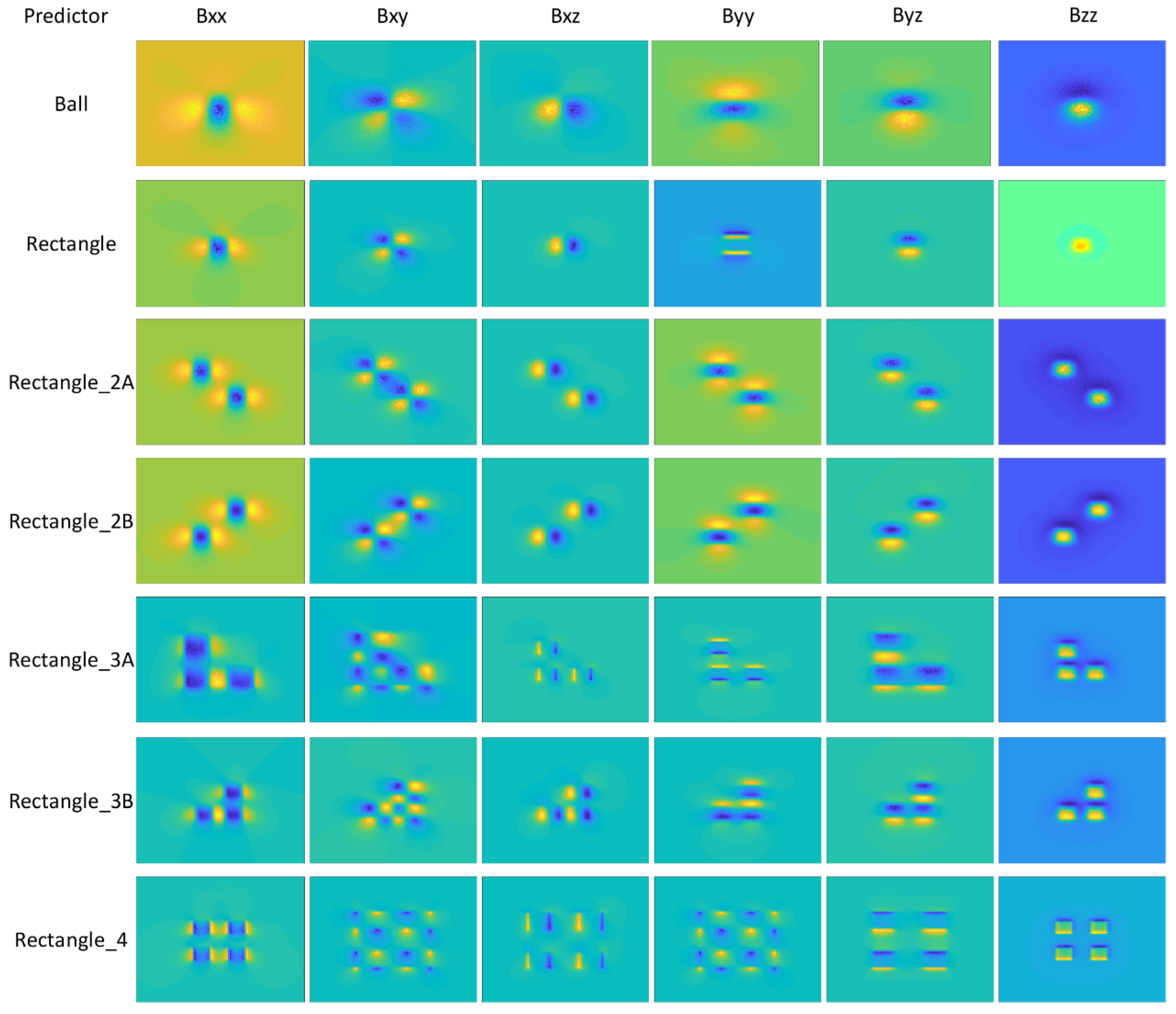
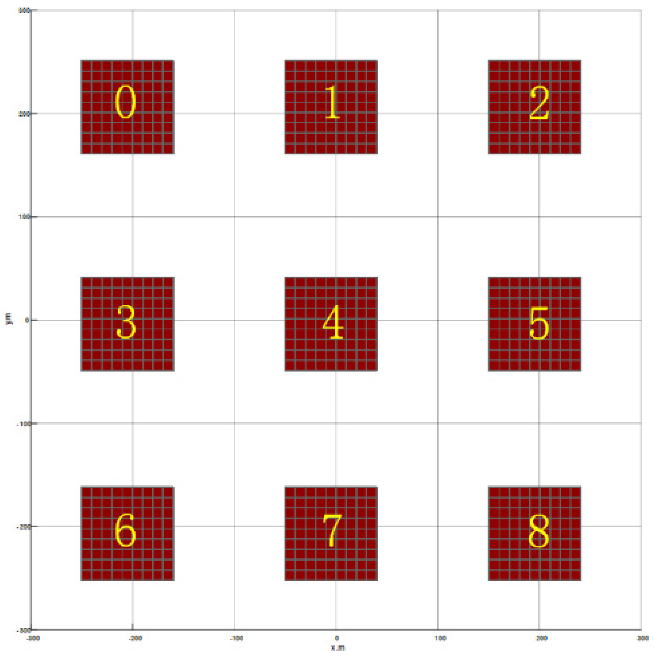
Each independent component of the MGT of all seven models is shown in Figure 5. The horizontal positions in the table are the numbering of the element positions (0 to 8) in a nine-grid matrix, as shown in Figure 6. The depth defined in the table is the depth from the center point to the surface. The magnetic declination (D), magnetic inclination (I) and magnetization susceptibility are physical parameters, where the unit of magnetization susceptibility is (SI). The effect of remanence is not considered separately in the model simulation and, if not stated, is considered as a whole.
To verify the feasibility of this method, we first set the dimensional range of the model within a space of 500 m. The main reason for this is to prevent the number of grids from being too large and increase the number of operations. The X-axis is the east-west axis and the positive direction is east, and thus the Y-axis is the north-south axis and the positive direction is north in the model area. The length, width and depth of the test area are all 400 m, which is within a shallow surface area, and the grid of the forward model is divided into 10 m × 10 m × 10 m cubes. Taking the B z z component of the MGT of the single-module Rectangle model as an example, the magnetic anomaly is a square body with 90 m side length and its initial center position is located at the center of the set area at coordinates (200, 200, 100). In order to simplify the model’s settings, all other magnetic anomalies are also modeled using the same single cube, with the center point of the test area as their symmetrically distributed center and the center point of the cube being in the horizontal plane with a depth of 100 m. For example, the Rectangle_4 model has 4 cubes symmetrically divided about the center point, and the two adjacent cubes are spaced 40 m apart in both X and Y directions.
The depth prediction range is set as 40 m–360 m with a step of 80 m, i.e., the depth prediction matrix is Equation (6), the magnetic declination (D) magnetic inclination (I) and magnetization susceptibility prediction range can be configured according to the prediction target. In this study, the prediction range of D is −10°~10° with a step of 2°, as in Equation (7); the prediction range of I is (52°–2°) with a step of 2°, as in Equation (8); and the prediction range of permeability is 0.1–0.6 (SI) with a step of 0.1, as in Equation (9):
Tag _ Depth = [ 40 120 200 280 360 ]
T a g _ D = [ 10 8 6 4 2 0 2 4 6 8 10 ]
T a g _ I = [ 52 56 58 60 62 64 66 68 70 72 ]
T a g _ M a g _ S u s = [ 0.1 0.2 0.3 0.4 0.5 0.6 ]

3.2. Sample Generation Algorithms

Taking the sample magnetic inclination (I) as an example, the predicted label set by Table 1 is T a g _ I [ 52 72 ] , the step is T a g _ I _ S t e p = 2 and then the label matrix is the prediction matrix shown in Equation (8). After determining the label matrix, the other physical parameters can be used to generate a random one-dimensional matrix using Equation (10):
P i = a + ( b a ) × r a n d ( N , 1 )     i [ 1 , m ]
where m is the type of the parameter and r a n d ( N , 1 ) is a row, N , and one column, a random matrix between (0~1). Combining the random matrices of each physical parameter, the integrated parameter matrix, as in Equation (11), is obtained:
P = [ P 1 P 2 P m ]
The matrix P is used as a loop variable and substituted into the tensor gradient forward modeling program to iteratively generate the required data sample size. The sample-producing algorithm’s process is shown in Algorithm 1.
Algorithm 1. Sample Produce
1:Procedure Sample (Tag_Station, Shape, Depth, Magnetic, Tag_I, Tag_D …)
2:e.g., Produce Tag_I
3:Initialize:  Tag_I ← [52 54 56 … 72] ∈ [52 72];   Species = 5;
4:Tag_Station ← [0 1 2  …  8];          Number > 8000;
5:Shape ← [Ball Rectangle Rectangle_2A Rectangle_2B …];
6:Depth ← [40 120 … 360];
7:Magnetic ← 0.1 + 0.6(0.6 − 0.1) × rand(m,1)      Magnetic ∈ [0.1 0.6]
8:Tag_D ← −10 + 10(10 + 10) × rand(n,1)       Tag_D ∈ [−10 10]
9:Components ← [Bxx Bxy Bxz Byy Byz Bzz];
10:Pi ← {Tag_Station, Shape, Depth, …}
11:while k1 < Number/Species do
12:while k2 < Number/Species do
13:  Sample_Tag_I(i)Mag_Tensor_Forword(P{k1,k2}, Components, …)
14:  Tag_Record(i) ← [P{k1,k2}, …]
15:      …
16:end While
17:end While
18:save Sample_Tage_I
19:saveTag_Record
20:endprocedure

3.3. Network Training and Prediction

According to the parameter configuration table and grid partitioning requirements in 3.1.1, we generate data samples for multiple models, and the number of samples for each type of model is 8000. In the training and testing process, we use the samples after randomly disordering them, with 60% of the samples used as the training set, 20% of the samples as the validation set and the remaining 20% of the samples as the test set.
The following is an example of the Rectangle model and Rectangle_2B model (shown in Figure 5), which both generate independent component samples with the same parameter settings, and their test set prediction accuracies are shown in Table 2 and Table 3.
The horizontal position and model recognition rate can reach 100% because the shape contour variability between the horizontal position and model samples is large among all components. In Figure 5 and Figure 6, the variability of the independent components of each model can be compared, and the position variability is obvious so it is very easy to identify.
The accuracy of depth prediction can reach more than 93%, thus ensuring the accuracy of magnetization susceptibility prediction. The change of both depth and magnetic susceptibility affects the change of magnetic field intensity. From the magnetic forward equation, Equation (1), it is known that the effect of depth on magnetic field intensity is twice as large as that of magnetic susceptibility and, if the magnetic susceptibility only changes in a small range, its change on magnetic field intensity is small relative to the change of depth and does not affect the prediction of depth. It is also understood that the change in magnetic field intensity caused by a small range of change in magnetic susceptibility relative to the change in depth on magnetic field intensity is considered a weak noise effect and can be ignored. In this study, we predict the depth first, and the depth value is known in the magnetization prediction, which in turn ensures the accuracy of the magnetization prediction.
Comparing Table 2 and Table 3, the prediction accuracy of the double square model is higher than that of the single square model, which is due to the fact that the former’s magnetic gradient tensor signal intensity is greater than that of the latter, under the same physical parameters, and contains more information on magnetic detail features.
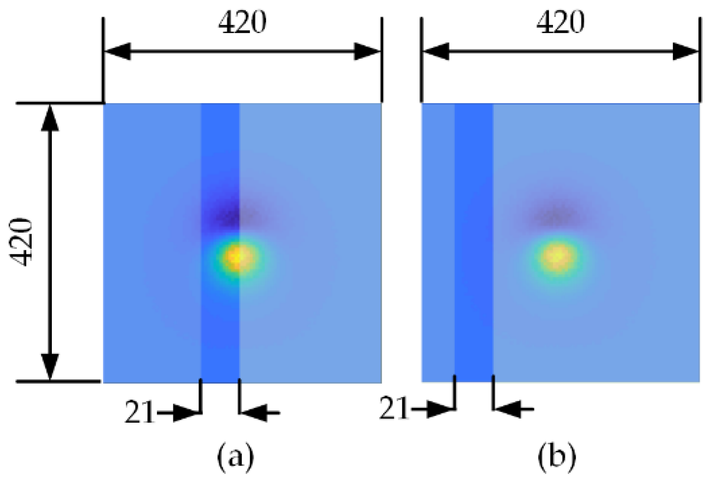
Under the assumption that the shape and size of the detection target are known, we attempt to extract the type and magnetic parameter information from the local part of the image sample and also test the generalization ability of the CNN. We perform a clipping test to predict the magnetic permeability with the B z z component of the Rectangle model. As shown in Figure 7, the normalized image sample size is 420 × 420 pixels; a section with a width of 21 pixels is selected, clipping the remaining width on both sides and leaving only the middle. The sample image’s size after clipping is 21 × 420. We select two different parts of the image to clip as examples: Figure 7a is clipped from the middle of the image and Figure 7b’s clipping is off-center.
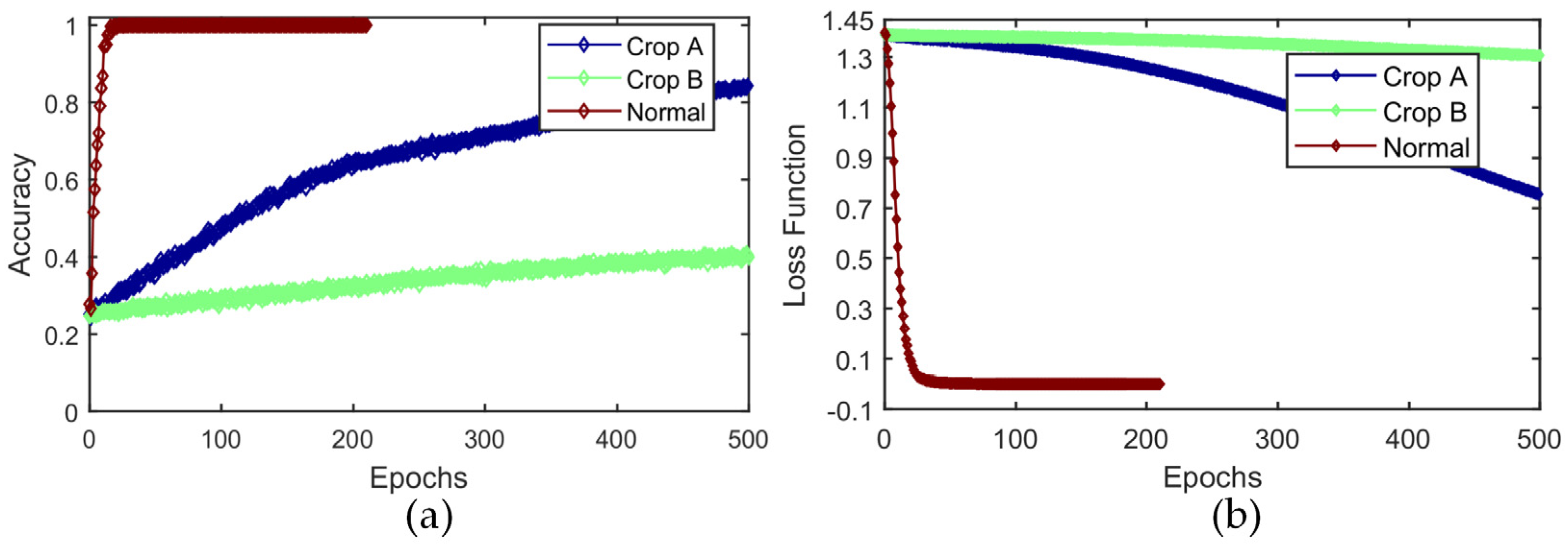
The test results are shown in Figure 8, where two sets of shear patterns and normal patterns, each showing the accuracy and loss degree comparisons in the neural network training process, from the comparison curve can be seen. Results indicate that: a) In the case of a suitable shear site (Figure 7a), the convergence speed decreases as the number of iterations increases, but a better prediction accuracy of 82% over 500 Epochs is achieved; b) it is difficult to ensure that prediction accuracy reaches the global prediction accuracy level; and c) the prediction accuracy is affected by the shear site. If the shear site does not contain the trend of the anomalous body change (Figure 7b), it leads to the training being unable to converge and the prediction accuracy being difficult to improve. As shown in Figure 8a, the number of iterations is 500 and its training accuracy is 42%. Of course, from another angle of analysis, we can also conclude that the local cut of the image can also achieve predictions, indicating that the CNN has strong recognition abilities. In the real case, shown later, the local clipping will be used for parameter prediction.

3.4. Parametric Synthesis

In this study, the parameters extracted from the MGT image samples are only single feature representations of the target body, but in order to obtain an overall model for inversion, all physical parameters need to be integrated. When the prediction of information such as model shape, depth and magnetization susceptibility is completed, the inverse model can be displayed directly on a map. In addition, the results of each predicted parameter can be used for correction of the inversion model, and the model becomes more accurate when more items of parameters are predicted. This is consistent with the principle of stepwise approximation in traditional inversion methods. The prediction of multiple magnetic parameters also facilitates the analysis of inverse model and input model errors, which will be presented in the subsequent error analysis.
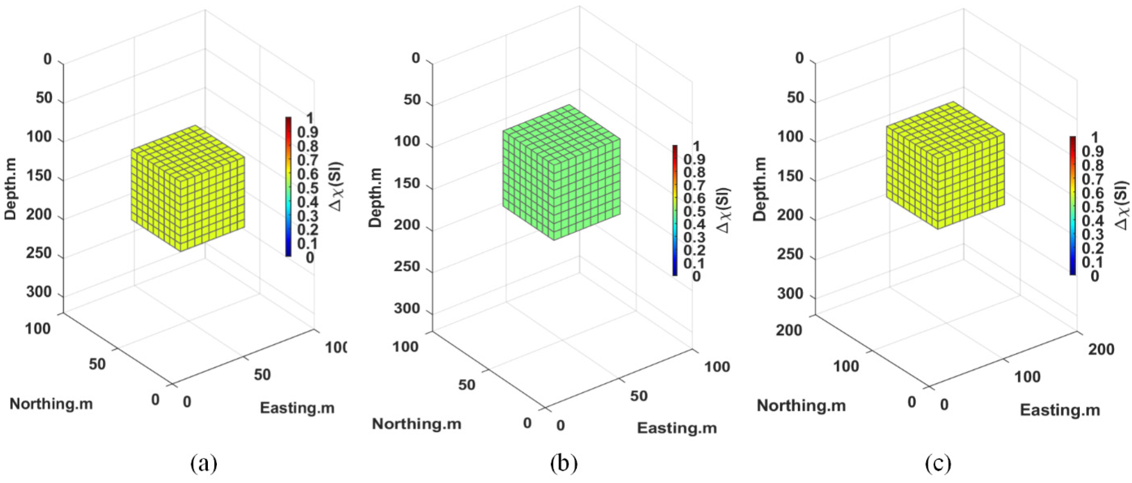
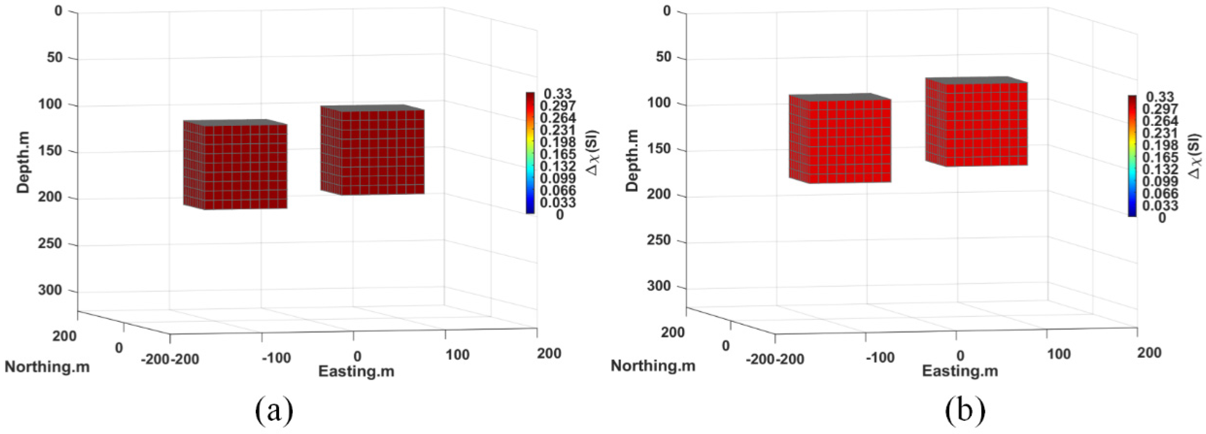
We continue to use the Rectangle and Rectangle_2B models as examples to predict the values of each parameter separately. Let the Rectangle model be a 90 m × 90 m × 90 m magnetic vein with a central depth of 150 m, a magnetization susceptibility of 0.6 (SI), a magnetic declination of −2° and a magnetic inclination of 58°. The size of the study area is 200 m × 200 m × 300 m in the x, y and z directions, respectively, as shown in Figure 9a. The Rectangle_2B model has two magnetic veins aligned at an angle of 45 degrees to the northwest, with a size of 90 m × 90 m × 90 m, veins 40 m apart in the horizontal and vertical directions, a central depth of 150 m, a magnetization susceptibility of 0.3 (SI), a magnetic declination of −2° and a magnetic inclination of 58° (shown in Figure 10a).
The overall inversion results after parameter synthesis are shown in Figure 9b,c and Figure 11b, where the overall inversion results of the Rectangle model are shown in Figure 9b,c. The inversion results of each independent component of the Rectangle_2B model are consistent, as shown in Figure 10b. From the model comparison plots, it can be seen that the overall inversion results of the MGT of each model match well with the real model, and it is difficult to distinguish their differences.
In the following Table 4 and Table 5, the results of the comparison of the real parameter values of the two input models with the prediction results of each component of the MGT are shown, respectively. Table 4 shows the comparison of the results for the Rectangle model; Table 5 shows the comparison of the results for the Rectangle_2B model. In the predicted results, the real depth value of the model is 150 m, but the predicted value is 120 m because the similarity between 150 m and the label value 120 m is greater than the similarity to label value 200 m. In the model Rectangle, the predicted results of the magnetic susceptibility of B x x and B y y differ from the true values by 0.1 (SI). The magnetization value of 0.33 (SI) in model Rectangle_2B is predicted to be 0.3 (SI) because the label with the greatest similarity to it is 0.3. This discontinuity in the label values, i.e., the span between the label values being too large, introduces a labeling error which is caused by the large span between the label values in the sample label definition. To reduce the labeling error introduced by the labels, a method of refining the label values can be adopted, i.e., increasing the number of labels and reducing the spacing between numerical labels.
Figure 11 and Figure 12 each show a 2D graphical comparison of the independent components of the MGT and the predicted components of the Rectangle model and Rectangle_2B model, respectively. The consistency of the profile of each component is good but there are also some differences, mainly that the magnetic field intensity of the predicted model component is larger than that of the real model, because the difference between the predicted depth and the real model is 30 m. In addition, from the forward modeling equation, Equation (1), it is known that depth has a greater effect on the magnetic field than magnetization susceptibility.
Table 6 and Table 7 show the Misfit error and MSE error of each independent component of the two prediction models above, and for each the Misfit is below 0.2 and the MSE is below 600. In addition, a comparison of the two models shows that the errors of the dual model’s components are generally higher than the errors of the single model’s components in this test. However, in Table 3 and Table 4, the prediction accuracy of the Rectangle_2B model is better than the Rectangle model. Comparing Table 4 and Table 5, we can find that the Magnetic susceptibility of Rectangle_2B model is 0.33 (SI), but the prediction value of each component is 0.3 (SI) with an error of 0.03 (SI). This situation is caused by the large step span of tag values and the low identification resolution, which ultimately leads to a high Misfit error and MSE error rate.
As shown in Figure 11 and Figure 12, and Table 6 and Table 7, to achieve MGT error analysis results for the inverse model, the inverse model needs to be forward modeled. This forward modeling requires geometry and depth, as well as information on physical parameters such as magnetic permeability, magnetic declination (D) and magnetic inclination angle (I). In conclusion, it is necessary to predict more magnetic parameters and to integrate multiple parameters in order to obtain inversion results that match closer to the measured magnetic target body.

3.5. Analysis of Factorsaffecting Prediction Accuracy

3.5.1. The Number of Training Samples

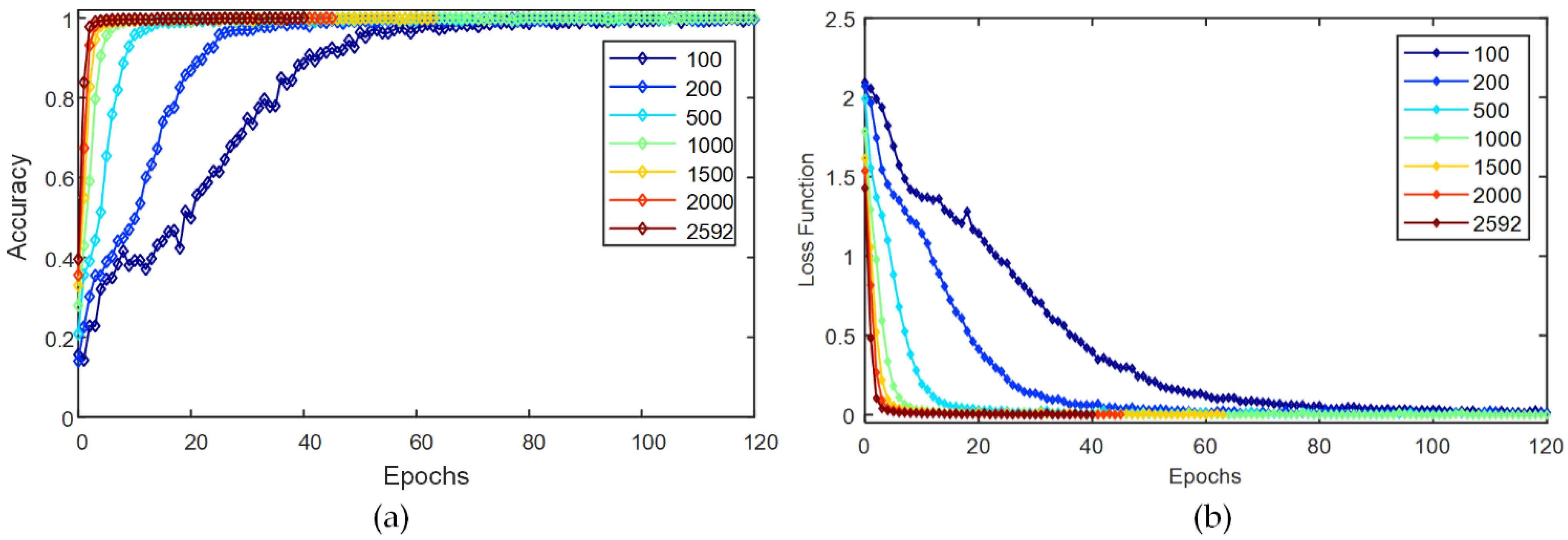
The number of training samples is the key to ensure the success of prediction. The neural network needs a certain number of samples in order to learn the difference information in each feature vector and thus perform classification. The following is an example of the Rectangle model’s B y y component being used to predict the magnetic declination (D). As shown in Table 1, the prediction range is −10°~10°, and the sample sizes of 100, 200, 500, 1000, 1500, 2000 and 2592 are taken for testing respectively. In addition, 1200 samples are randomly selected from the remaining samples for the accuracy test set. Figure 13 shows the training loss rate and training accuracy comparison graphs. Table 8 shows the single Epoch time, the number of iterations to reach 90% accuracy, and the accuracy of the accuracy test set for each case.
Through testing, we find that increasing the number of samples can improve the convergence speed and accuracy of the predicted test set. However, when the number of samples reaches a certain number, each sample’s contribution to the improvement of prediction accuracy decreases which also leads to the increase of single-Epoch times and longer training time. In this test, the best time-efficiency and accuracy requirements are reached when the number of samples in a single category is from 500 to 1000. When high prediction accuracy can be achieved with fewer samples, it indicates the strong learning ability of the CNN, and secondly, it also reflects the low variability of sample features and the existence of feature homogenization. This situation can reduce the number of samples, which has some implications for the methods needed to generate high-quality samples.

3.5.2. Sample Noise Levels

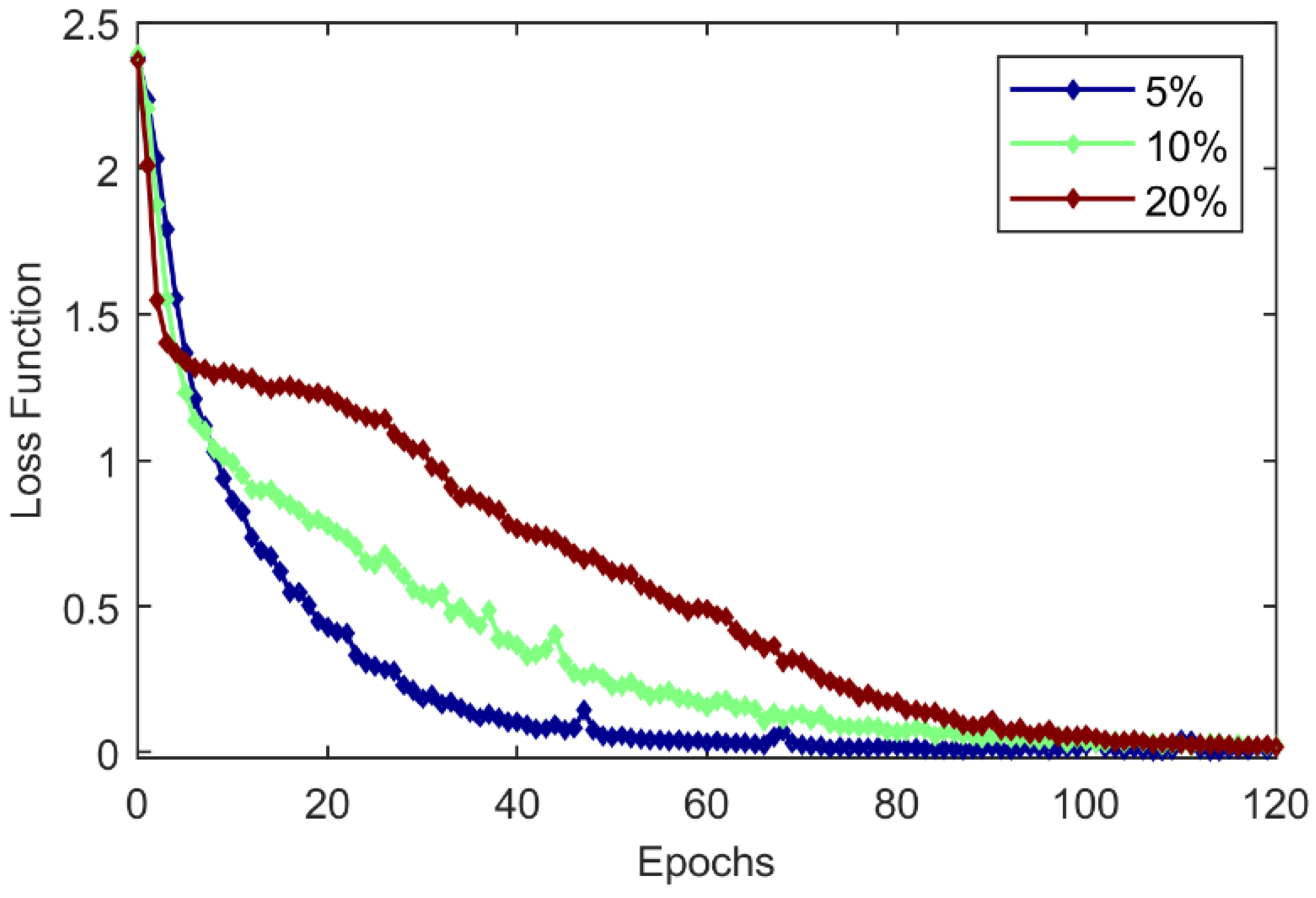
The sample noise affects the convergence speed during the training of the neural network, which is essentially an effect on the accuracy of the neural network’s sample feature extraction, but the prediction accuracy tends to be consistent when a sufficient number of training Epochs is reached. We take the Rectangle_2B model’s B z z component to predict the magnetic permeability (D) as an example, with 5%, 10% and 20% noisy samples for training, and all the parameter settings in the model remain the same except for the difference in noise level. As shown in Figure 14, the loss of the low-noise samples decreases faster than that of the high-noise samples throughout the training period, and the minimum loss rate is reached faster. That is, the noise metrics of the samples are inversely proportional to the rate of decline of the loss function. In the early training period, in the interval of 0~5 Epochs, the high-noise-level samples decline faster than the low-noise-level samples, after which the loss curves appear as intersection points. In the middle of training, between 5 and 100 Epochs, the high-noise-level samples decline less rapidly than the low-noise-level samples, and the low-noise-level samples reach their lowest loss range in the middle and late stages, and the change rate tends to be 0. In the late stage of training, between 100 and 120 Epochs, all three reach their lowest loss range and the loss curves overlap. According to the noise test curve comparison characteristics, the samples’ noise levels and data-quality levels can be evaluated.

3.5.3. MGT Joint Inversion

The MGTs have six different independent components to predict separately, and the joint prediction of multiple components can be achieved by statistical or weighting methods to obtain the best prediction accuracy; that is, the single-component prediction results can be corrected by the prediction results of the overall component, thus improving fault tolerance. For example, when less than half of the MGT components’ prediction values are wrong, the accuracy of the final prediction results can be ensured by methods such as the statistical or weighted averaging of each component.
We take the Rectangle_2B model as an example and use the neural network trained with the total magnetic field and each MGT component to predict the magnetic inclination (I). In order to ensure the consistency of the prediction results, all parameters in the model are set in the same range, except for the magnetic inclination (I). The output of the CNN’s results is in the form of predicted probability values, where the maximum probability value is obtained for each label.
Table 9 shows the prediction results for the inclination I = 62°. In this prediction test, 5% random noise is added, and the prediction accuracy is greater than 95%. The maximum predicted probability value of B x z in the table is 95.4%, which is lower than 99.99%. The predicted values of B x z components can also be ignored here, and the predicted values of other components are taken as the final results of the joint prediction. The accuracy of multi-component combined prediction is higher than that of single-component prediction.

4. Application to Field Data: Tallawang Magnetite Silica, Australia

4.1. Geologic Background

The Tallawang magnetite diorite deposit is located 18 km northwest of Gulgong in New South Wales (NSW), Australia, as shown in Figure 7 of Schmidt et al. (2004) [4]. It is located along the western margin of the Gulgong granite body, within the Lachlan folded belt, Hill End Trough stratigraphic sequence, in eastern Australia [59,60,61].
The magnetite was intruded during the attenuated phase of the Kanimblan orogeny in the late Carboniferous [62,63,64]. Mineralization occurred mainly in the Late Silurian-age Dungeree volcanic rocks (zircon uranium-lead isotopic age 418 million years), which are located on the margin of a deformed, matted particulate amphibolite intrusive body (Gurgaon granite body) that was intruded during the Late Carboniferous Kanimblan orogeny, and magnetite is thought to be reflected in the crystalline body [65,66,67].
The tectonically misshapen, deformed pod-like, semi-massive magnetite bodies show a steep dip to the west on the contact of the granitic saprolite bodies. It is also complicated by lateral faulting of a tightly folded host rock sequence (the Tarkan Formation), causing east-west displacement of the magnetite zone.
Numerous drill holes have been drilled around the magnetite body and the rock magnetism of the magnetite has been well characterized. The maximum magnetization of the test sample is 3.8 SI, with a remanence time of 40 a.m. −1 and a Koenigsberger ratio (Qs) of about 0.2 ~ 0.5. The remanence’s average orientation is WNW and steeply upward. The effective magnetization intensity, projected onto the vertical plane with the perpendicular, is steeply upward-oriented [4]. The local magnetic inclination (I) is −63.3°, the magnetic declination (D) is 11.37°, the total background magnetic field is 56,481 nT and the magnetite anomaly has an amplitude of 12,000 nT. The magnetite xenolith deposit is mostly vein-like, with a depth of about 10 m at the top and 120 m at the bottom.
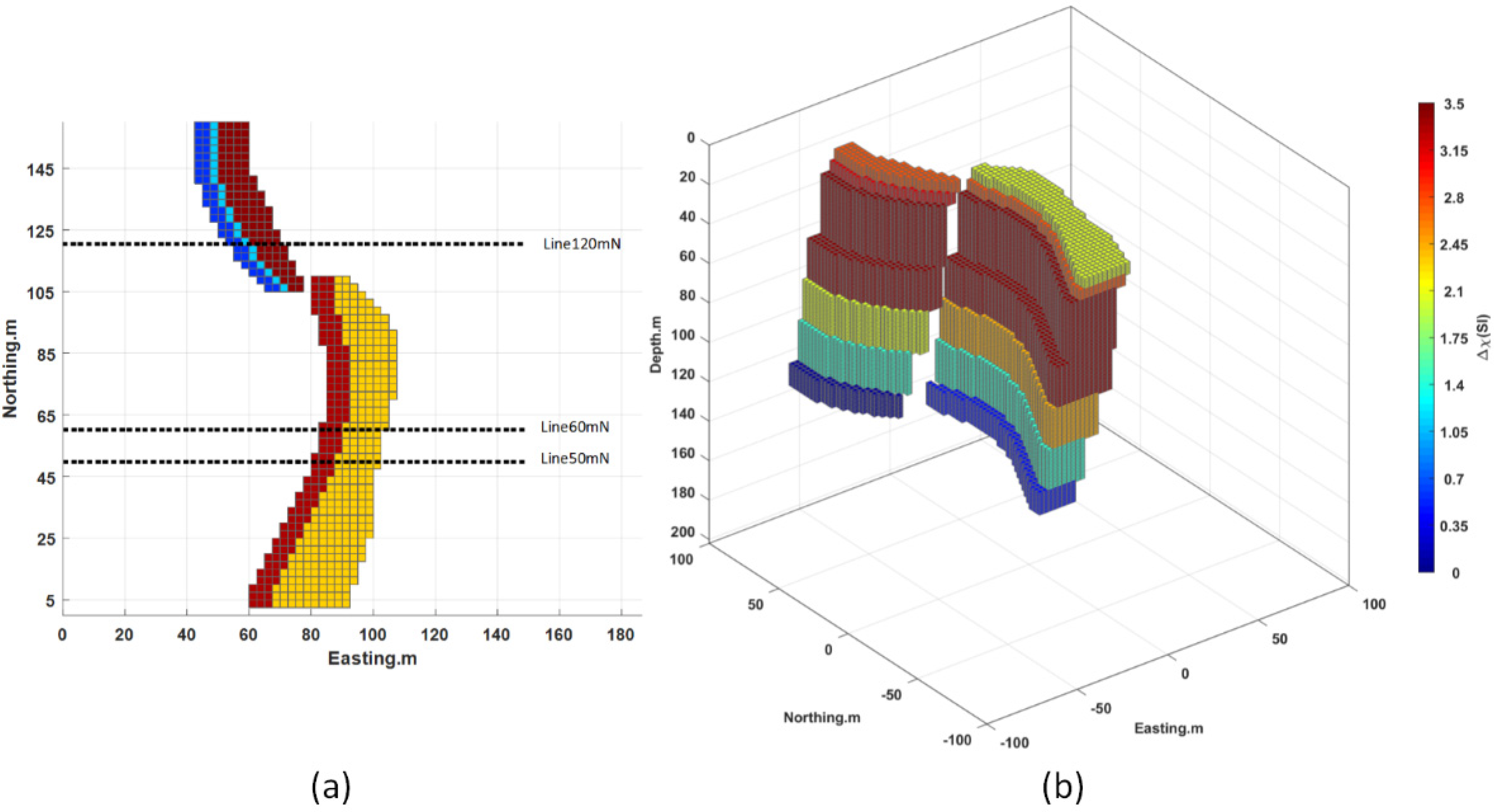
Schmidtet [4] demonstrated CSIRO’s GETMAG system’s performance on this magnetite skarn deposit in a field trial with three profiles (50 mN, 60 mN and 120 mN). The length of the measurement line is 150 m, shown in Figure 15, approximately perpendicular to the strike of the sillimanite deposit, reducing blending and effectively making the measurements two-dimensional and planar. The GETMAG system consists of three high-temperature superconducting quantum interference sensors independently spinning along a central axial direction, operating in liquid nitrogen (−196 °C) with the overall combination of an umbrella-shaped magnetic gradiometer device.
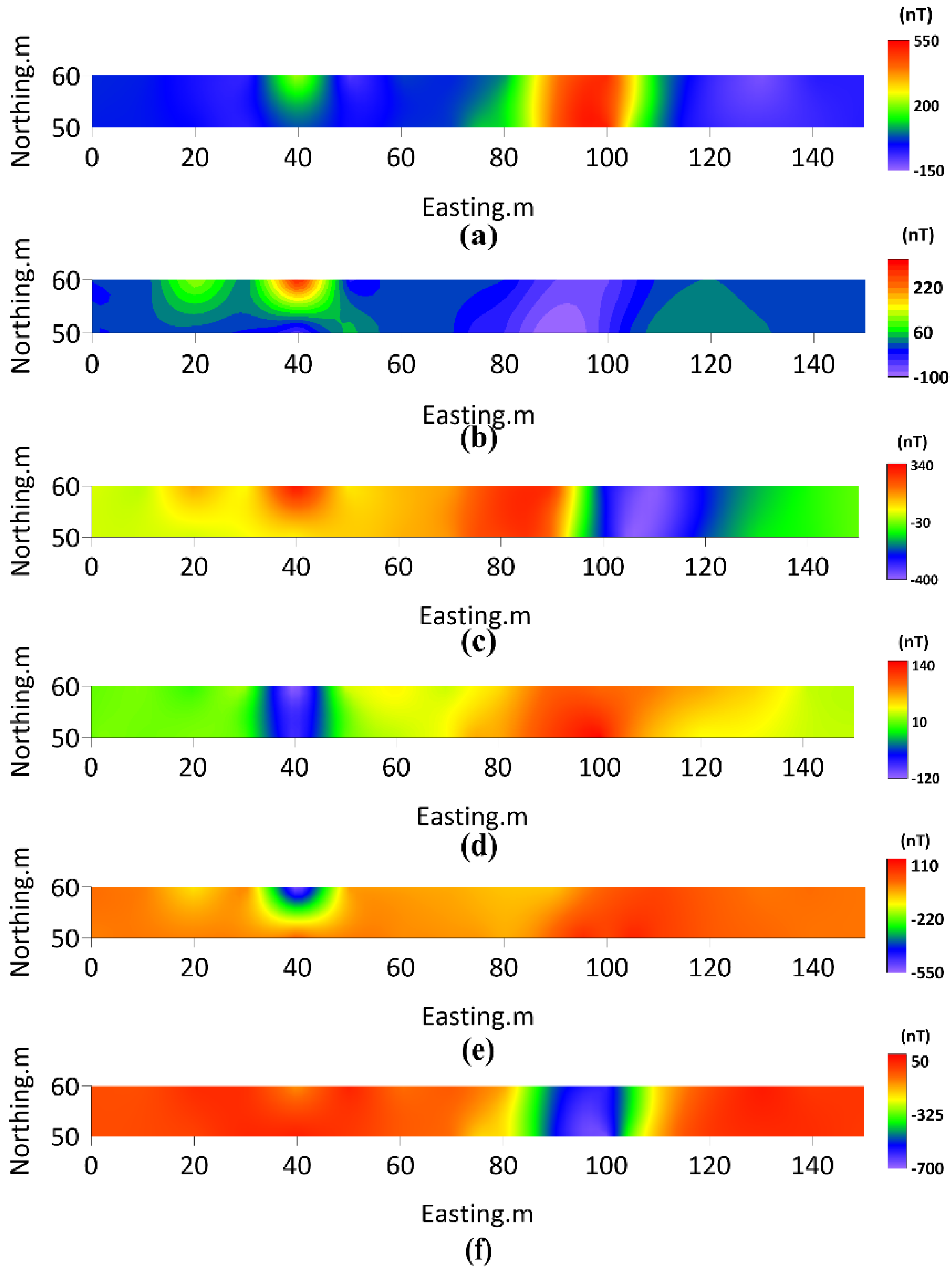
In Figure 15, the 50 mN, 60 mN and 120 mN lines all cross the magnetite vein, but the 120 mN and 60 mN lines are far apart and contain an east-west-northwest fault. There is not enough line data to reflect the real mine morphology, so we only take the two-dimensional plan composed of the 50 mN and 60 mN line data for local prediction and inversion interpretation, as shown in Figure 16.

4.2. Parameter Prediction

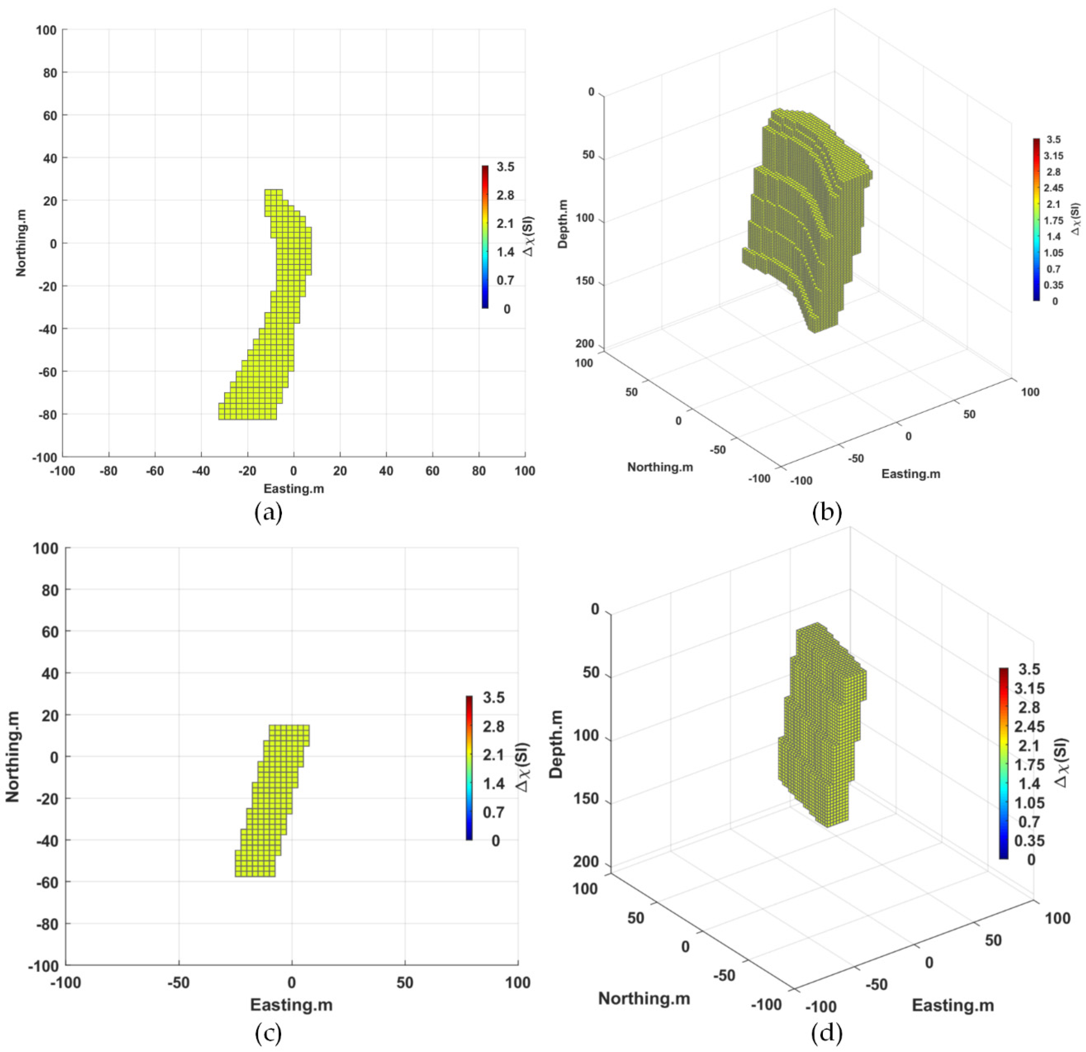
With reference to the orientation of the two test lines in Figure 15, we construct two example prediction models, the arc tilt model and the rhombohedral tilt model (Figure 17), for the magnetic rock vein crossed by the line. The vein is located 10 m underground, and the horizontal section is a northeast- and then northward-curved rock surface, as shown in Figure 17a, with a length and width of 107 m × 14 m. The x-axis (east is positive) extends from 72 m to 97 m, the y-axis (north is positive) extends from 0 m to 107 m, the z-axis (bottom is positive) extends from 120 m to the depth and with a westward tilt, as shown in Figure 17b. The horizontal cross-section is a northeast trapezoidal rock face, as shown in Figure 17c, with a length and width of 107 m × 14 m. The x-axis (east) extends from 72 m to 97 m, the y-axis (north) extends from 0 m to 107 m and the z-axis is buried at a depth of 120 m with a westward slope, as shown in Figure 17d.
The arc tilted magnetic dikes model and the rhombohedral tilted magnetic dikes model, with the same configuration of physical parameters, are configured with the following parameters: an I prediction range of −80°~80° with a step of 10°; a D prediction range of −170°~170° with a step of 10°; the magnetic anomaly is considered as a uniform magnetic body; the magnetic susceptibility prediction range is 1~3.5 (SI) with a step of 0.5 SI; and the depth of the center point of the magnetic body is -20 m. In addition, these two example models are used for shape prediction, together with the seven simulation models in Figure 5.

4.3. The Effect of the Source Body Parameters on Predictions

We predict each parameter of magnetite sillimanite ore with joint multi-component prediction, where the shape prediction results in an arc-shaped inclined body, which is consistent with magnetic iron ore dikes. The geometry of the magnetic anomalies is generally predicted by the B z z component, and we can find from Figure 5 that the B z z sample magnetic anomalies are clearly separated from the interface. In addition, the B z z component is suitable for the identification of a magnetic anomalous body shape that does not overlap in the vertical direction, as shown in Figure 16f.
The predicted depth of the center of the magnetic anomaly is 85 m, which is close to the actual depth of 55 m in the center of the magnetite silica. The depth has a large influence on the magnetic field intensity, and after unifying the color scale for samples with different depth values, the image differences are obvious and easy to identify.
The predicted value of magnetic inclination (I) is −50° for the B x x component, −70° for the B y z component and −60° for the B z z component. Combining the above three components, the predicted range of magnetic inclination (I) is [−50°, 70°], and its middle value of −60° is taken as the predicted value. The average direction of the magnetite residue is WNW, and for its effective magnetization intensity, all of which are in the steep upward direction, it can be concluded that the I of the remanence is upward and negative and then, combined with the local background magnetic field inclination, is −63.3°, so the predicted value (−60°) is consistent with the actual situation.
The predicted magnetic declination (D) is 50° for the B x x component, 170° for the B x z component, 30° for the B y y component, 170° for the B y z component and 170° for the B z z component. Combining the predicted values of the above components, the magnetic declination is positive, the predicted values with excessive deviation (30° and 50°) are removed and the final predicted value is 170°. From the B x x and B z z component plots in Figure 16a,f, respectively, through the center of the vein (within the interval of 80 m-110 m of the X-axis), the two sides of the vein are not completely symmetrical, the western value is smaller than the eastern value, it can be seen from the plots that the green diffusion range value on the left side of the B x x component is larger than the right side and the yellow diffusion range value on the left side of the B z z component is larger than the right side. In the case of negative magnetic inclination (I), compared to the forward modeling simulation results, we can see that the magnetic declination is positive and greater than 90°. In the geological background, the vein’s total field values are all positive and the predicted value of 170° is consistent with the actual situation when the geological background magnetic declination is 11.37°.
The magnetite sillimanite body is considered as a homogeneous magnet with a predicted central depth of 85 m. The label value corresponding to the predicted maximum probability value of the magnetization of each independent component is 1 (SI). The magnetite sillimanite has a maximum magnetization of 3.8 (SI) and its overall average magnetization decreases. The predicted value of 1 (SI) is consistent with the overall uniform magnetization range within the mine.
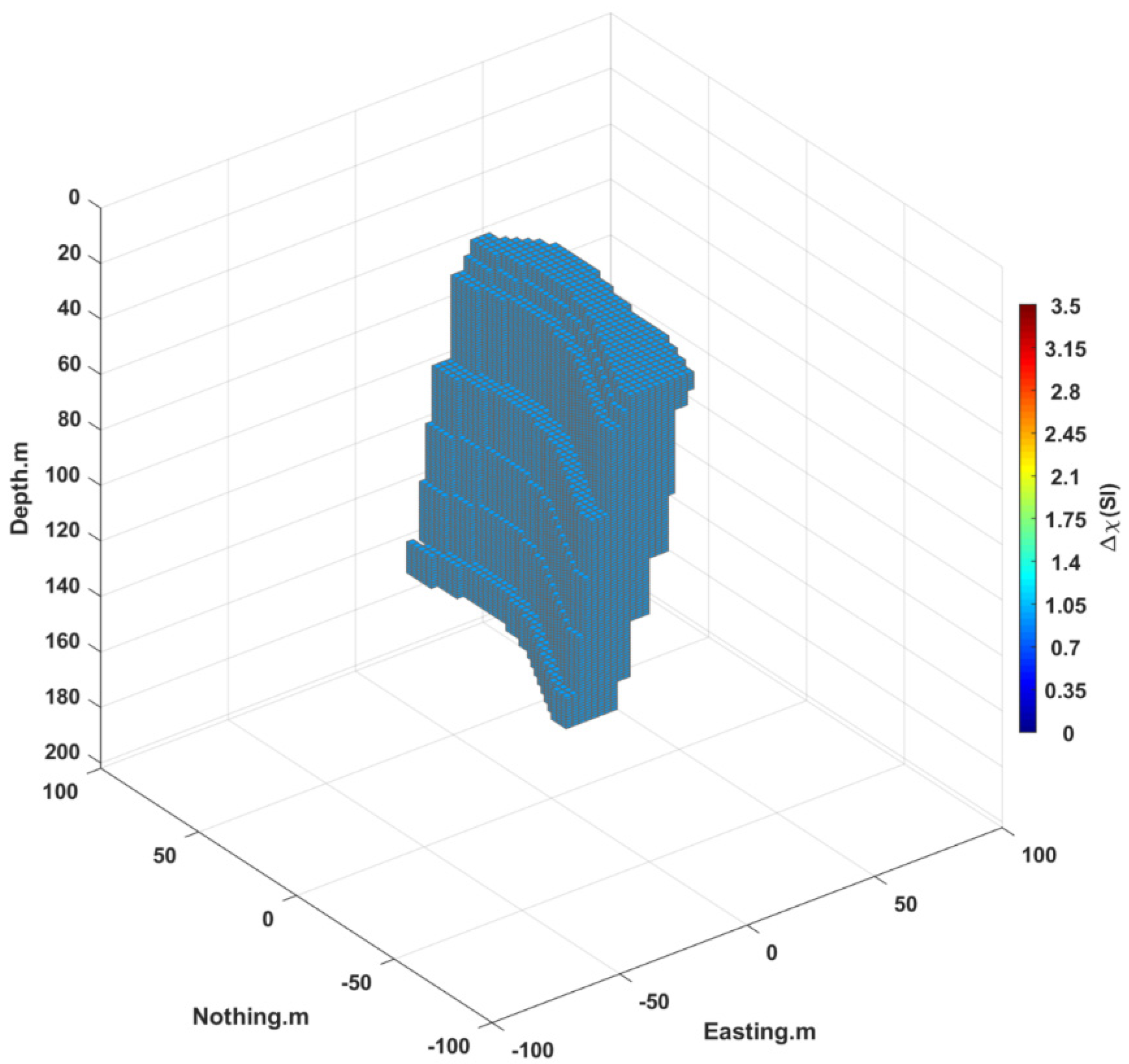
Combining the predicted parameters above, the inversion result of magnetite sillimanite is an arc-shaped slab vein inclined to the west with a depth of 85 m at its center, a magnetic inclination of −60°, a magnetic declination of 170° and a uniform magnetization of 1 (SI), as shown in Figure 18.
In the measurement area, there is an outcrop with line number 60 mN with its front end adjacent to the outcrop, as shown in Figure 16; in the range of 35 m~45 m on the X-axis, there is a semicircular anomaly with interference information, but it does not affect the prediction results because the constructed real measurement model is empty in the outcrop area, which indicates that, through the construction of the model area, the CNN can realize the designation of the prediction area and suppress the noise interference in the non-prediction area to realize its function, similar to the local fixed-point focus.

5. Conclusions

By training on a large number of image samples generated by a synthetic model, a CNN can be used to extract magnetic parameters, synthesize all magnetic parameters and then achieve an inversion model of MGT data. In this work, we develop a CNN-based 3D inversion method for MGT data. We use randomly generated image samples of each independent component of the MGT for the classification and identification of geometric shape information and physical parameters of magnetic gradient detection data of magnetic target bodies. We also investigate a method of identifying the geometric shape and depth first and then further identifying the physical property parameters, and this stepwise identification method can suppress the influence of uncertainties and improve the recognition rate. We validate our optimized CNN inversion network by two synthetic models and shear model comparison tests, and prove that the geometric shape and magnetic parameter information of a magnetic target body can be effectively recognized by the trained CNN. In this study, it is found that the discontinuity of CNN classification labels can cause the illusion of large actual errors and falsely high prediction accuracy. The MGT data span a large magnitude and are severely polarized. With a uniform color scale display of the sample set, samples with weak MGT signals are blurred during imaging and fail to present their overall features, which affects the image imaging quality and leads to a lower recognition rate or even failure to converge in training. It is necessary to reduce the spacing of adjacent label values, refine the range of label values or resort to other auxiliary methods in order to improve the recognition rate.
The uncertainty analysis shows that sample noise can be suppressed by increasing the number of iterations, and the change characteristics of the training loss rate curve reflect the noise level of the samples. When the amount of training samples reaches a certain number, prediction accuracy and training time reach their best state; in this test, 500~1000 training samples of each category reach the best state. With higher numbers, the prediction accuracy remains the same but the training time is longer. In addition, multi-component joint prediction is more advantageous than single-component prediction because the prediction error rate is reduced.
We also apply the developed method to the inversion of MGT data from the Tallawang magnetite diorite deposit in Australia. The depth of burial of the magnetite centroids in the measured area and the information of related magnetic parameters are predicted from the data of two measured lines.
Although we have verified that a CNN can achieve MGT inversion by testing, this partial testing does not necessarily indicate that this method is better than the traditional inversion method. In the case of complex target bodies with anomalous and anisotropic structures, more matching models need to be constructed to expand the training sample pool and more time is needed for the preliminary model construction and sample generation compared to the traditional inversion method; therefore, both have mutual advantages, which means that CNN inversion can be considered as a complement to the traditional magnetic field inversion method.
In future research, in order to balance prediction accuracy and effectiveness, developing a more lightweight prediction model is an important direction for MGT inversion based on machine learning.

6. Patents

This achievement has been submitted to the State Intellectual Property Office of the People’s Republic of China for an invention patent named “A method and apparatus for 3D magnetic gradient tensor inversion based on CNN”. The application number is: 202210372621.7.

Author Contributions

Conceptualization, H.D. and X.H.; methodology, H.D.; software, H.D.; validation, H.D., H.C., S.L., R.P., Y.L. and B.H.; investigation, H.D., H.C., S.L., R.P., Y.L. and B.H.; formal analysis, H.D., H.C., S.L., R.P., Y.L. and B.H.; supervision, X.H.; project administration, X.H.; funding acquisition, X.H. All authors have read and agreed to the published version of the manuscript.

Funding

This research was supported by MOST Special Fund from the State Key Laboratory of Geological Processes and Mineral Resources, China University of Geosciences, grant number MSFGPMR01-4.

Acknowledgments

We are grateful to Chen Longwei of Guilin University of Technology for his analysis of the observed data, which provides an in-depth analysis of the D and I for the strong remanent magnetization environment.

Conflicts of Interest

The authors declare no conflict of interest.

References

  1. Christensen, A.; Rajagopalan, S.J.P. The magnetic vector and gradient tensor in mineral and oil exploration. Preview 2000, 84, 77. [Google Scholar]
  2. Schmidt, P.; Clark, D.A. Advantages of measuring the magnetic gradient tensor. Preview 2000, 85, 26–30. [Google Scholar]
  3. Heath, P.; Heinson, G.; Greenhalgh, S. Some comments on potential field tensor data. Explor. Geophys. 2003, 34, 57–62. [Google Scholar] [CrossRef]
  4. Schmidt, P.; Clark, D.; Leslie, K.; Bick, M.; Tilbrook, D.; Foley, C. GETMAG—A SQUID magnetic tensor gradiometer for mineral and oil exploration. Explor. Geophys. 2004, 35, 297–305. [Google Scholar] [CrossRef]
  5. Schmidt, P.W.; Clark, D.A. The calculation of magnetic components and moments from TMI: A case study from the Tuckers igneous complex, Queensland. Explor. Geophys. 1998, 29, 609–614. [Google Scholar] [CrossRef]
  6. Stolz, R.; Zakosarenko, V.; Schulz, M.; Chwala, A.; Fritzsch, L.; Meyer, H.-G.; Köstlin, E.O. Magnetic full-tensor SQUID gradiometer system for geophysical applications. Lead. Edge 2006, 25, 178–180. [Google Scholar] [CrossRef]
  7. Schmidt, P.W.; Clark, D.A. The magnetic gradient tensor: Its properties and uses in source characterization. Lead. Edge 2006, 25, 75–78. [Google Scholar] [CrossRef] [Green Version]
  8. Meyer, H.; Stolz, R.; Chwala, A.; Schulz, M. SQUID technology for geophysical exploration. Phys. Status Solidi (C) 2005, 2, 1504–1509. [Google Scholar] [CrossRef]
  9. Li, Y.; Oldenburg, D.W. 3-D inversion of gravity data. Geophysics 1998, 63, 109–119. [Google Scholar] [CrossRef]
  10. Li, Y.; Oldenburg, D.W. 3-D inversion of magnetic data. Geophysics 1996, 61, 394–408. [Google Scholar] [CrossRef]
  11. Frahm, C.P. Inversion of the magnetic field gradient equation for a magnetic dipole field. NCSL Informal Rep. 1972, 135–172. [Google Scholar]
  12. Wynn, W.; Frahm, C.; Carroll, P.; Clark, R.; Wellhoner, J.; Wynn, M. Advanced superconducting gradiometer/Magnetometer arrays and a novel signal processing technique. IEEE Trans. Magn. 1975, 11, 701–707. [Google Scholar] [CrossRef]
  13. Zhang, C.; Mushayandebvu, M.F.; Reid, A.B.; Fairhead, J.D.; Odegard, M. Euler deconvolution of gravity tensor gradient data. Geophysics 2000, 65, 512–520. [Google Scholar] [CrossRef] [Green Version]
  14. Zhdanov, M.S. Geophysical Inverse Theory and Regularization Problems; Elsevier: Amsterdam, The Netherlands, 2002; Volume 36. [Google Scholar]
  15. Zhdanov, M.; Ellis, R.; Mukherjee, S. Three-dimensional regularized focusing inversion of gravity gradient tensor component data. Geophysics 2004, 69, 925–937. [Google Scholar] [CrossRef]
  16. Zhdanov, M.; Liu, X.; Wilson, G. Potential field migration for rapid 3D imaging of entire gravity gradiometry surveys. First Break 2010, 28, 47–51. [Google Scholar] [CrossRef]
  17. Cai, H. Migration and Inversion of Magnetic and Magnetic Gradiometry Data. Master’s Thesis, The University of Utah, Salt Lake City, UT, USA, 2012. [Google Scholar]
  18. Sun, J.; Li, Y. Multidomain petrophysically constrained inversion and geology differentiation using guided fuzzy c-means clustering. Geophysics 2015, 80, ID1–ID18. [Google Scholar] [CrossRef]
  19. Zhdanov, M.S.; Lin, W. Adaptive multinary inversion of gravity and gravity gradiometry data. Geophysics 2017, 82, G101–G114. [Google Scholar] [CrossRef]
  20. Liu, S.; Hu, X.; Zhang, H.; Geng, M.; Zuo, B. 3D Magnetization Vector Inversion of Magnetic Data: Improving and Comparing Methods. Pure Appl. Geophys. 2017, 174, 4421–4444. [Google Scholar] [CrossRef]
  21. Geng, M.; Hu, X.; Zhang, H.; Liu, S. 3D inversion of potential field data using a marginalizing probabilistic method. Geophysics 2018, 83, G93–G106. [Google Scholar] [CrossRef]
  22. Raiche, A. A pattern recognition approach to geophysical inversion using neural nets. Geophys. J. Int. 1991, 105, 629–648. [Google Scholar] [CrossRef] [Green Version]
  23. Spichak, V.; Popova, I. Artificial neural network inversion of magnetotelluric data in terms of three-dimensional earth macroparameters. Geophys. J. Int. 2000, 142, 15–26. [Google Scholar] [CrossRef]
  24. Sun, J.; Li, Y. Joint inversion of multiple geophysical and petrophysical data using generalized fuzzy clustering algorithms. Geophys. J. Int. 2016, 208, 1201–1216. [Google Scholar] [CrossRef]
  25. Singh, A.; Sharma, S. Identification of different geologic units using fuzzy constrained resistivity tomography. J. Appl. Geophys. 2018, 148, 127–138. [Google Scholar] [CrossRef]
  26. Puzyrev, V. Deep learning electromagnetic inversion with convolutional neural networks. Geophys. J. Int. 2019, 218, 817–832. [Google Scholar] [CrossRef] [Green Version]
  27. Noh, K.; Yoon, D.; Byun, J. Imaging subsurface resistivity structure from airborne electromagnetic induction data using deep neural network. Explor. Geophys. 2020, 51, 214–220. [Google Scholar] [CrossRef]
  28. Liu, B.; Guo, Q.; Li, S.; Liu, B.; Ren, Y.; Pang, Y.; Guo, X.; Liu, L.; Jiang, P. Deep Learning Inversion of Electrical Resistivity Data. IEEE Trans. Geosci. Remote Sens. 2020, 58, 5715–5728. [Google Scholar] [CrossRef] [Green Version]
  29. Yang, Q.; Hu, X.; Liu, S.; Jie, Q.; Wang, H.; Chen, Q. 3-D Gravity Inversion Based on Deep Convolution Neural Networks. IEEE Geosci. Remote Sens. Lett. 2021, 19, 3001305. [Google Scholar] [CrossRef]
  30. Nurindrawati, F.; Sun, J. Predicting Magnetization Directions Using Convolutional Neural Networks. J. Geophys. Res. Solid Earth 2020, 125, e2020JB019675. [Google Scholar] [CrossRef]
  31. Li, R.; Yu, N.; Wang, X.; Liu, Y.; Cai, Z.; Wang, E. Model-Based Synthetic Geoelectric Sampling for Magnetotelluric Inversion With Deep Neural Networks. IEEE Trans. Geosci. Remote Sens. 2020, 60, 4500514. [Google Scholar] [CrossRef]
  32. Hu, Z.; Liu, S.; Hu, X.; Fu, L.; Qu, J.; Wang, H.; Cheng, Q. Inversion of magnetic data using deep neural networks. Phys. Earth Planet. Inter. 2021, 311, 106653. [Google Scholar] [CrossRef]
  33. He, S.; Cai, H.; Liu, S.; Xie, J.; Hu, X. Recovering 3D Basement Relief Using Gravity Data Through Convolutional Neural Networks. J. Geophys. Res. Solid Earth 2021, 126, e2021JB022611. [Google Scholar] [CrossRef]
  34. Krizhevsky, A.; Sutskever, I.; Hinton, G.E. ImageNet classification with deep convolutional neural networks. NIPS 2012, 60, 84–90. [Google Scholar] [CrossRef]
  35. Li, K.; Chen, L.-W.; Chen, Q.-R.; Dai, S.-K.; Zhang, Q.-J.; Zhao, D.-D.; Ling, J.-X. Fast 3D forward modeling of the magnetic field and gradient tensor on an undulated surface. Appl. Geophys. 2018, 15, 500–512. [Google Scholar] [CrossRef]
  36. Gao, X.; Sun, S. Comment on “3DINVER. M: A MATLAB program to invert the gravity anomaly over a 3D horizontal density interface by Parker-Oldenburg’s algorithm”. Comput. Geosci. 2019, 127, 133–137. [Google Scholar] [CrossRef]
  37. Ren, Z.; Chen, C.; Tang, J.; Chen, H.; Hu, S.; Zhou, C.; Xiao, X. Closed-form formula of magnetic gradient tensor for a homogeneous polyhedral magnetic target: A tetrahedral grid example. Geophysics 2017, 82, WB21–WB28. [Google Scholar] [CrossRef]
  38. Blakely, R.J. Potential Theory in Gravity and Magnetic Applications; Cambridge University Press: Cambridge, UK, 1995. [Google Scholar] [CrossRef]
  39. Beiki, M.; Clark, D.A.; Austin, J.R.; Foss, C.A. Estimating source location using normalized magnetic source strength calculated from magnetic gradient tensor data. Geophysics 2012, 77, J23–J37. [Google Scholar] [CrossRef] [Green Version]
  40. Schmidhuber, J. Deep learning in neural networks: An overview. Neural Netw. 2015, 61, 85–117. [Google Scholar] [CrossRef] [Green Version]
  41. Hinton, G.E.; Salakhutdinov, R.R. Reducing the Dimensionality of Data with Neural Networks. Science 2006, 313, 504–507. [Google Scholar] [CrossRef] [Green Version]
  42. LeCun, Y.; Bengio, Y.; Hinton, G. Deep learning. Nature 2015, 521, 436–444. [Google Scholar] [CrossRef]
  43. Zayernouri, M.; Karniadakis, G.E. Fractional Sturm-Liouville eigen-problems: Theory and numerical approximation. J. Comput. Phys. 2013, 252, 495–517. [Google Scholar] [CrossRef]
  44. Chen, X.; Duan, J.; Karniadakis, G.E. Learning and meta-learning of stochastic advection–diffusion–reaction systems from sparse measurements. Eur. J. Appl. Math. 2021, 32, 397–420. [Google Scholar] [CrossRef]
  45. Lu, L.; Jin, P.; Karniadakis, G.E. DeepONet: Learning nonlinear operators for identifying differential equations based on the universal approximation theorem of operators. arXiv 2019, arXiv:1910.03193. [Google Scholar]
  46. Nair, V.; Hinton, G.E. Rectified linear units improve restricted boltzmann machines. In Proceedings of the 27th International Conference on Machine Learning (ICML-10), Haifa, Israel, 21–24 June 2010; pp. 807–814. [Google Scholar]
  47. Han, J.; Moraga, C. The influence of the sigmoid function parameters on the speed of back-propagation learning. In From Natural to Artificial Neural Computation; Springer: Berlin/Heidelberg, Germany, 1995; pp. 195–201. [Google Scholar]
  48. Kingma, D.P.; Ba, J. Adam: A method for stochastic optimization. In Proceedings of the International Conference Learn (ICLR), San Diego, CA, USA, 5–8 May 2015. [Google Scholar]
  49. Clevert, D.-A.; Unterthiner, T.; Hochreiter, S. Fast and accurate deep network learning by exponential linear units (elus). arXiv 2015, arXiv:1511.07289. [Google Scholar]
  50. Xu, B.; Wang, N.; Chen, T.; Li, M. Empirical Evaluation of Rectified Activations in Convolutional Network. arXiv 2015, arXiv:1505.00853. [Google Scholar]
  51. Srivastava, N.; Hinton, G.; Krizhevsky, A.; Sutskever, I.; Salakhutdinov, R. Dropout: A simple way to prevent neural networks from overfitting. J. Mach. Learn. Res. 2014, 15, 1929–1958. [Google Scholar]
  52. Loshchilov, I.; Hutter, F. SGDR: Stochastic gradient descent with restarts. arXiv 2016, arXiv:1608.03983. [Google Scholar]
  53. Hinton, G.; Srivastava, N.; Swersky, K. Neural networks for machine learning lecture 6a overview of mini-batch gradient descent. Cited On 2012, 14, 2. [Google Scholar]
  54. He, T.; Zhang, Z.; Zhang, H.; Zhang, Z.; Xie, J.; Li, M.; Recognition, P. Bag of Tricks for Image Classification with Convolutional Neural Networks. arXiv 2019, arXiv:1812.01187. [Google Scholar]
  55. Wiegert, R.; Oeschger, J. Generalized Magnetic Gradient Contraction Based Method for Detection, Localization and Discrimination of Underwater Mines and Unexploded Ordnance. In Proceedings of the OCEANS 2005 MTS/IEEE, Washington, DC, USA, 17–23 September 2005; Volume 1322, pp. 1325–1332. [Google Scholar]
  56. Blakely, R.J.; Simpson, R.W. Approximating edges of source bodies from magnetic or gravity anomalies. Geophysics 1986, 51, 1494–1498. [Google Scholar] [CrossRef]
  57. Wijns, C.; Perez, C.; Kowalczyk, P. Theta map: Edge detection in magnetic data. Geophysics 2005, 70, L39–L43. [Google Scholar] [CrossRef]
  58. Pilkington, M.; Tschirhart, V. Practical considerations in the use of edge detectors for geologic mapping using magnetic data. Geophysics 2017, 82, J1–J8. [Google Scholar] [CrossRef]
  59. Seccombe, P.K.; Offler, R.; Ayshford, S. Origin of the Magnetite Skarn at Tallawang, NSW Preliminary Sulfur Isotope Results. In Research Report 1995–2000; IAEA: Vienna, Austria, 2000. [Google Scholar]
  60. Offler, R.; Seccombe, S.A.P. Geology and origin of the Tallawang magnetite skarn, Gulgong, NSW. In Proceedings of the 3rd National Conference of the Specialist Group in Economic Geology, Launceston, Australia, 10–14 November 1997. [Google Scholar]
  61. Ayshford, S.; Offler, R.; Seccombe, P. Geology and origin of the Tallawang magnetite skarn, Gulgong, NSW. Geol. Soc. Aust.-Abstr. 1997, 44, 5. [Google Scholar]
  62. Foster, D.A.; Gray, D.R. Evolution and Structure of the Lachlan Fold Belt (Orogen) of Eastern Australia. Annu. Rev. Earth Planet. Sci. 2000, 28, 47–80. [Google Scholar] [CrossRef]
  63. Collins, W.; Vernon, R. Palaeozoic arc growth, deformation and migration across the Lachlan Fold Belt, southeastern Australia. Tectonophysics 1992, 214, 381–400. [Google Scholar] [CrossRef]
  64. Lu, J.; Seccombe, P.; Foster, D.; Andrew, A. Timing of mineralization and source of fluids in a slate-belt auriferous vein system, Hill End goldfield, NSW, Australia: Evidence from 40Ar39Ar dating and O- and H-isotopes. Lithos 1996, 38, 147–165. [Google Scholar] [CrossRef]
  65. Powell, C.M.; Edgecombe, D.R.; Henry, N.M.; Jones, J.G. Timing of regional deformation of the hill end trough: A reassessment. J. Geol. Soc. Aust. 1976, 23, 407–421. [Google Scholar] [CrossRef]
  66. Packham, G.H. Radiometric evidence for Middle Devonian inversion of the Hill End Trough, northeast Lachlan Fold Belt. Aust. J. Earth Sci. 1999, 46, 23–33. [Google Scholar] [CrossRef]
  67. Colquhoun, G.P. Siliciclastic sedimentation on a storm- and tide-influenced shelf and shoreline: The Early Devonian Roxburgh Formation, NE Lachlan Fold Belt, southeastern Australia. Sediment. Geol. 1995, 97, 69–98. [Google Scholar] [CrossRef]
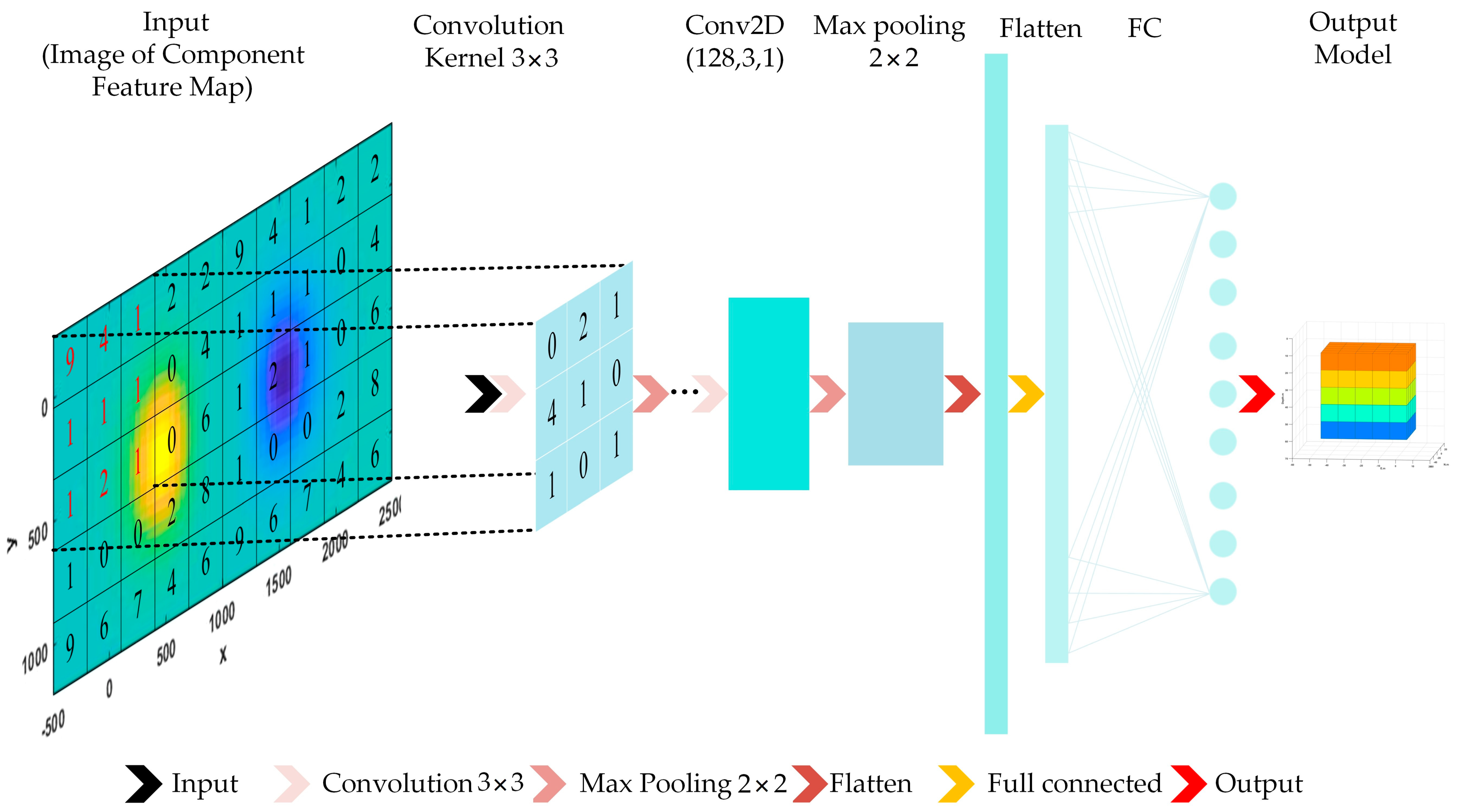
Figure 1. CNN framework schematic.
Minerals 12 00566 g001
Figure 2. Optimized AlexNet network architecture.
Minerals 12 00566 g002
Figure 3. Schematic diagram of the MGT CNN inversion process.
Minerals 12 00566 g003
Figure 4. Steps of the prediction process.
Minerals 12 00566 g004
Figure 5. 2D images of seven models of MGT components.
Minerals 12 00566 g005
Figure 6. The test area is divided into 9 grid areas on a 3 × 3 equally spaced grid and numbered in order, from left to right and top to bottom. The labeled numbers 0–8 are defined as the different horizontal and vertical positions’ point numbers.
Minerals 12 00566 g006
Figure 7. Clipping different parts across the image. (a) Crossing the middle line. (b) Far from the center line (the blue area in the figure is the clipping area).
Minerals 12 00566 g007
Figure 8. Comparison of prediction results of two cutting methods for graphical samples. (a) Train Accuracy. (b) Train Loss.
Minerals 12 00566 g008
Figure 9. Comparison of inversion results. (a) Input model: Rectangle; (b) B x x and B y y inversion result; and (c) B x y , B x z , B y z and B z z inversion result.
Minerals 12 00566 g009
Figure 10. Comparison of inversion results. (a) Input model: Rectangle_2B; (b) B x x , B x y , B x z , B y y , B y z and B z z inversion result.
Minerals 12 00566 g010
Figure 11. Comparison of the Rectangle model’s components and prediction model’s components. (af) are the B x x , B x y , B x z , B y y , B y z and B z z components of the Rectangle model; (gm) are the B x x , B x y , B x z , B y y , B y z and B z z components of the prediction model.
Minerals 12 00566 g011
Figure 12. Comparison of the Rectangle_2B model’s components and prediction model’s components. (af) are the B x x , B x y , B x z , B y y , B y z and B z z components of the Rectangle_2B model; (gm) are the B x x , B x y , B x z , B y y , B y z and B z z components of the prediction model.
Minerals 12 00566 g012
Figure 13. Result comparison. (a) Accuracy of training and (b) loss rate comparison.
Minerals 12 00566 g013
Figure 14. Training loss at different sample noise levels.
Minerals 12 00566 g014
Figure 15. Geology of the Tallawang magnetite skarn. Test line is 50 mN, 60 mN, 120 mN. (Redraw from Schmidt et al., 2004) [4]. (a) Plane graph; (b) Sheer plan.
Minerals 12 00566 g015
Figure 16. Plot of independent component data for each of the 50 mN and 60 mN measurement lines. (a) B x x ; (b) B x y ; (c) B x z ; (d) B y y ; (e) B y z ; and (f) B z z (Data from Schmidt et al., 2004) [4].
Minerals 12 00566 g016
Figure 17. Example models. (a) Planar graph of an arc tilted magnetic vein, (b) section view of an arc tilted magnetic vein, (c) planar graph of a rhomboidal tilted magnetic vein, and (d) section view of a rhomboidal tilted magnetic vein.
Minerals 12 00566 g017
Figure 18. Side view of the 3D inversion model of magnetite sillimanite.
Minerals 12 00566 g018
Table 1. Model types and parameter variation ranges.
ShapeTag NameHorizontal PositionDepth (m)DIMagnetic Su-Sceptibility(SI)
Minerals 12 00566 i001Ball(0,8)(40,360)(−10,10)(52,72)(0.1,0.6)
Minerals 12 00566 i002Rectangle(0,8)(40,360)(−10,10)(52,72)(0.1,0.6)
Minerals 12 00566 i003Rectangle_2A(0,8)(40,360)(−10,10)(52,72)(0.1,0.6)
Minerals 12 00566 i004Rectangle_2B(0,8)(40,360)(−10,10)(52,72)(0.1,0.6)
Minerals 12 00566 i005Rectangle_3A(0,8)(40,360)(−10,10)(52,72)(0.1,0.6)
Minerals 12 00566 i006Rectangle_3B(0,8)(40,360)(−10,10)(52,72)(0.1,0.6)
Minerals 12 00566 i007Rectangle_4(0,8)(40,360)(−10,10)(52,72)(0.1,0.6)
Table 2. Model prediction accuracies of Rectangle.
PredictorBxxBxyBxzByyByzBzz
Horizontal Position100% 100% 100% 100% 100% 100%
Shape100% 100% 100% 100% 100% 100%
Depth93.1%96.2%94.1%99.9%98.9%95.8%
D93.6%92.2%91.1%99.9%97.9%94.2%
I99.9%99.4%98.7%99.9%99.8%99.4%
Magnetic Sus-ceptibility(SI)91.4%90.2%92.7%91.1%90.5%93.3%
Table 3. Model prediction accuracies of Rectangle_2B.
PredictorBxxBxyBxzByyByzBzz
Horizontal Position100% 100% 100% 100% 100% 100%
Shape100% 100% 100% 100% 100% 100%
Depth99.1%99.2%99.1%99.9%99.3%99.9%
D99.9%99.9%99.9%99.9%99.9%99.9%
I99.6%99.4%99.7%99.9%99.4%99.3%
Magnetic Sus-ceptibility(SI)99.3%99.7%99.3%99.9%99.8%99.1%
Table 4. The Rectangle model’s parameter settings and prediction results for each independent component.
PredictorInput
Model
Magnetic Tensor Gradient Prediction
BxxBxyBxzByyByzBzz
Horizontal Position4444444
ShapeRectangleRectangleRectangleRectangleRectangleRectangleRectangle
Depth150120120120120120120
D−2°−2°−2°−2°−2°−2°−2°
I58°58°58°58°58°58°58°
Magnetic Sus-
ceptibility(SI)
0.6 0.5 0.6 0.6 0.5 0.6 0.6
Table 5. Model Rectangle_2B parameter settings and prediction results of each independent component.
PredictorInput
Model
Magnetic Tensor Gradient Prediction
BxxBxyBxzByyByzBzz
Horizontal Position4444444
ShapeRectan
gle_2B
Rectan
gle_2B
Rectan
gle_2B
Rectan
gle_2B
Rectan
gle_2B
Rectan
gle_2B
Rectan
gle_2B
Depth150120120120120120120
D−2°−2°−2°−2°−2°−2°−2°
I58°58°58°58°58°58°58°
Magnetic Sus-
ceptibility(SI)
0.330.30.30.30.30.30.3
Table 6. Rectangle model‘s prediction Misfit and MSE.
Error PatternBxxBxyBxzByyByzBzz
Misfit0.07070.05800.03540.06370.03460.2676
MSE197.54259.04151.25190.98147.95180.38
Table 7. Rectangle_2B model’s prediction Misfit and MSE.
Error PatternBxxBxyBxzByyByzBzz
Misfit0.10170.07370.05800.06690.06010.1212
MSE622.11498.66310.91482.59333.51591.29
Table 8. Test Results Statistics.
Sample NumbersT_ Epoch(s) 1Epoch_Num 2T_Sum(s) 3Test Accuracy
10044417697.3%
20092421699.5%
500181018099.8%
100035517599.9%
1500664264100%
2000883264100%
25921143342100%
1 T_Epoch is the number of seconds consumed during each Epoch, 2 Epoch_Num is the number of iterations needed to reach 90% accuracy, and 3 T_Sum is the number of seconds consumed to reach 90% accuracy.
Table 9. Comparison of the prediction accuracies of the total magnetic field and the MGT.
Component Name5860626466
Bt1.48 × 10−81.26 × 10−79.91 × 10−11.46 × 10−131.76 × 10−4
Bxx2.09 × 10−149.57× 10−189.99 × 10−11.61 × 10−313.67× 10⁻⁴
Bxy4.28 × 10−139.91× 10−169.99 × 10−12.63 × 10−283.91 × 10⁻⁴
Bxz1.11 × 10−184.87 × 10−119.54 × 10−12.87 × 10−242.59 × 10⁻⁸
Byy3.05 × 10−132.19 × 10−139.99 × 10−11.65 × 10−253.16 × 10⁻⁵
Byz4.06 × 10−153.95 × 10−139.99 × 10−17.01 × 10−237.64 × 10⁻⁶
Bzz1.74 × 10−101.77 × 10−109.99 × 10−12.02 × 10−187.53 × 10⁻⁵
Publisher’s Note: MDPI stays neutral with regard to jurisdictional claims in published maps and institutional affiliations.