Improving Inversion Quality of IP-Affected TEM Data Using Dual Source

Abstract

The induced polarization (IP) effects in transient electromagnetic (TEM) responses pose difficulties to the TEM data interpretation and inversion. The IP effects break the monotony in TEM decay curves and can even cause sign reversals and lead to the singularity and non-monotony of inversion. The singularity problem is still urgent to be solved. In this paper, the forward modeling method of IP-affected TEM responses is developed using the Cole–Cole model and a frequency-time domain transformation. A TEM data acquisition scheme using a dual-source method without a significant increase in field work is proposed to weaken the singularity and improve the inversion quality finally. Based on the modeling and analysis, the dual-source scheme is designed to guarantee all stations be measured twice with different loops. The joint inversion of dual-source datasets is realized by using an objective combing function and the particle swarm optimization (PSO) algorithm. The synthetic data test proved the validity of the algorithm and illustrated that the joint dual-source method greatly weakened the singularity and stabilized the inversion. The field example of the Baiyun golden deposit showed well consistency with resistivity logging and TEM logging results and predicted the gold mineralization below 2000 m.

1. Introduction

The transient electromagnetic method (TEM) has been widely used in metallic mineral exploration, geological survey, and other prospecting fields as an effective geophysical technique [1,2,3,4,5,6,7,8]. Conventionally, TEM data are interpreted based on the assumption that the earth is purely resistive. The resistivity distribution of the stratum can be obtained by methods including TEM response analysis [9,10], apparent resistivity definition [11,12,13], and inversions [14,15,16,17,18]. However, due to the widespread polarizable medium [19,20] (typically, graphite and sulfide), the earth has inherent dispersion properties [21,22,23,24,25]. With the electromagnetic field propagating, the induced polarization (IP) response will occur in the stratum and superimpose on the TEM response. The superposition will distort the normal attenuation of TEM response or even cause sign reversals [26,27]. It brings difficulties and interference to TEM data processing and finally leads to incorrect interpretations [28].

The physical mechanism of the IP effect in TEM response can be explained by some simplified theories, such as the interaction of two polarizable circuits [29]. The process of the IP effect that occurs in TEM response can be divided into two stages [30]. The first stage is the charge stage, which starts immediately after the primary field turnoff. The induced electromotive force is strong and decreases rapidly. The polarizable medium is charged by the induced eddy current (TEM current), and the IP voltage increases slowly. The IP and the TEM current are in the same direction at this stage. When the IP voltage exceeds the induced electromotive force, the charge stage ends, and the second stage, i.e., the discharge stage, begins. At this stage, the IP current has an opposite direction to the TEM current, and a negative TEM response may occur.

The forward modeling of the IP-affected TEM response is mainly based on the Cole–Cole complex conductivity model [19], which is widely used in electromagnetic exploration. The asymptotic analytical solution of polarizable uniform ground excited by a loop has been derived, and the distortion of TEM response caused by the IP effect has been proved [31]. Forward modeling of layered earth has been realized by time-frequency conversion [26,32], and the TEM response of a complex 3D model considering the IP effect has been simulated by numerical algorithms such as integral equation and finite difference method [33,34]. The previous simulations have shown the complexity of IP-affected TEM response.

Various identification, separation, and interpretation methods of IP effects in TEM have been developed to handle the IP-affect TEM data [35,36,37]. Generally, the identification methods delineate polarizable bodies by the spatial range of sign reversals that occur. The separation methods always separate IP responses from TEM responses using basis function fitting and sign constraint methods, and then the pure TEM responses are inverted to obtain the resistivity of the earth. The TEM-IP joint inversion method can recover the resistivity and polarization parameters simultaneously and has the best applicability and accuracy. However, the joint inversion has a strong singularity and non-monotony due to the complexity of IP-affected TEM responses and more unknowns, which results in difficult convergence of the linear inversion algorithm and algebraic non-uniqueness. Zhi et al. proposed a global optimization inversion strategy using the particle swarm optimization algorithm, which preliminarily solved the convergence difficulty caused by non-monotonic IP-affected TEM response [38]. Kozhevnikov et al. proposed a joint inversion method [39,40], the TEM responses were observed at the same station twice using central loop and coincident loop configurations with different side lengths, respectively, and then the two datasets were combined for joint inversion. A survey station was observed by central loop configuration with 200 m × 50 m loop and coincident loop configuration with 50 m × 50 m loop successively in their experiment, and the inversion combining the two TEM datasets showed higher recover rates of geoelectrical parameters than the inversion using single dataset directly. The method can provide additional data constraints and weaken the singularity problem of inversion. However, the combination of different configurations requires two transmitting loops with different sizes to be laid out at each survey station, and the measurement needs to be repeated twice, which brings notably supernumerary field work.

The main goal of the method proposed in this paper is to weaken the singularity of the inversion of TEM data considering the IP effect without a significant increase in field work, and then obtain the resistivity and polarization parameters of the earth synchronously. We first outline the problems caused by the singularity of inversion and discuss the methods to weaken the singularity. A dual-source configuration is proposed to acquire IP-affected TEM datasets under different excitation conditions. Then the joint inversion strategy is adopted to obtain the resistivity and polarization parameters of the earth. Previous studies have shown the necessity to utilize a global optimization algorithm on account of the complex non-monotony of IP-affected TEM responses. The particle swarm optimization algorithm is a novel population-based search algorithm that simulates cooperative society behaviors. It has attracted a lot of attention because of its advantages of easy implementation, high accuracy, and fast global convergence. Its superiority and good performance in solving practical problems have been shown in our previous papers [38]. Hence, particle swarm optimization is adopted for global optimization of the joint inversion in this paper. Finally, synthetic and field examples are tested to verify the effectiveness of the algorithm.

2. Materials and Methods

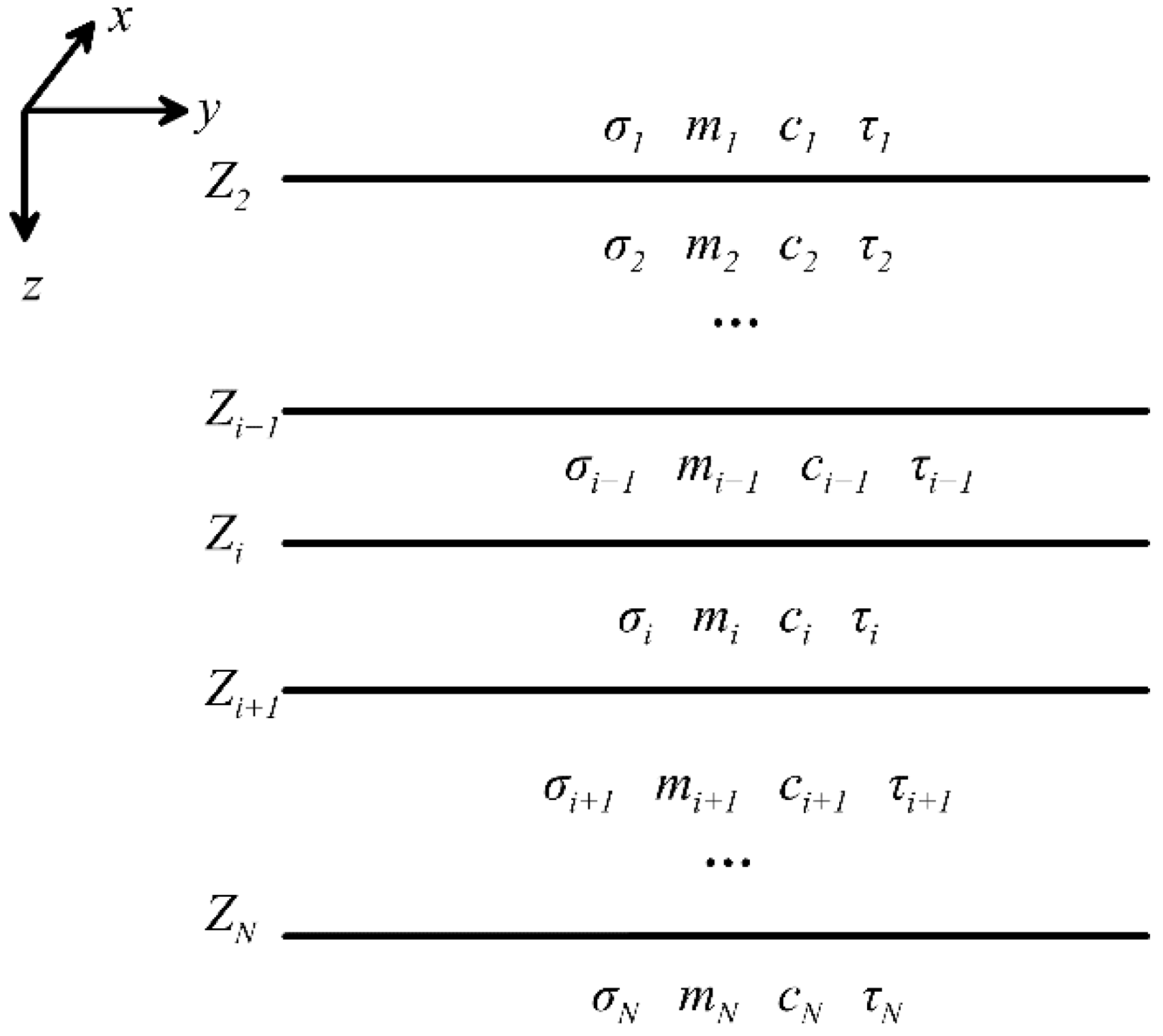
2.1. Forward Modeling of IP-Affected TEM Response

The forward modeling of electromagnetic response is performed in the frequency domain first, and then the response is converted to the time domain by the discrete sine transform. The IP effect of the earth is described by the Cole–Cole complex conductivity model [19]:

$${\sigma }^{*}(\omega )={\sigma }_0\frac{1+{(j\omega \tau )}^c}{1+(1-m){(j\omega \tau )}^c}$$

(1)

where j is the imaginary unit, and j² = −1; ω represents the angular frequency; σ₀ represents conductivity of the earth at zero-frequency; m represents the chargeability, and 0 ≤ m ≤1; c represents the exponent describing the variation of phase with frequency, and 0 ≤ c ≤ 1; τ represents the IP relaxation time constant.

The layered earth model and right-handed Cartesian coordinate system are established as Figure 1. The layers are uniquely determined by their electrical parameters (σ_i, m_i, c_i, τ_i) and the z-coordinate of its top interface Z_i. Assuming a time-harmonic factor of e^−iωt, the governing equations can be written as

$$\nabla \times E=\mathrm{i}\omega B$$

(2)

$$\nabla \times B=\mu \sigma E+\mu J$$

(3)

where B represents the magnetic field, E represents the electric field, μ represents the permeability, and J represents the source current density vector. The magnetic vector potential A in the Coulomb gauge ∇·A = 0 can be expressed by

$$B=\nabla \times A$$

(4)

$$E=\mathrm{i}\omega A+\frac{1}{\mu \sigma }\nabla (\nabla ·A)$$

(5)

Considering the model shown in Figure 1 excited by an electric dipole, the magnetic vector potential can be obtained by Hankel transformation [41]:

$$A(r)=\frac{1}{2\pi }{\displaystyle {\int }_0^{\infty }\widehat{A}}(\lambda ,z){\mathrm{J}}_0(\lambda r)\lambda \mathrm{d}\lambda$$

(6)

where J₀ is the 0-order Bessel functions of the first kind, r is the separation of the receiver from the dipole source, r is the position vector from the dipole source to the receiver. The kernel $\widehat{A}$ can be obtained by recursion of each layer, and then the electromagnetic fields E and B in the frequency domain can be obtained using Equations (4) and (5).

The transient electromagnetic responses are obtained by Fourier transform. For the widely used step waveform:

$$I(t)=\{\begin{array}{l}{I}_0 t<0\hfill \\ 0 t>0\hfill \end{array}$$

(7)

the corresponding Fourier transform pair is:

$$\{\begin{array}{l}F(\omega )={\displaystyle {\int }_{-\infty }^{\infty }f}(t)e^{i\omega t}d\omega \hfill \\ f(t)=\frac{1}{2\pi }{\displaystyle {\int }_{-\infty }^{\infty }F}(\omega )e^{-i\omega t}d\omega \hfill \end{array}$$

(8)

where F(ω) represents the response in the frequency domain, and f(t) represents the response in the time domain. When considering the symmetry of the real and imaginary parts of F(ω), f(t) can be obtained by sine transformations in the real number field. A double precision 160-point digital filter with high precision and fast calculation speed are adopted to carry out sine transform in this paper, and the transient electromagnetic response of the arbitrary shape source is calculated by the electric dipole superposition technique [38].

The forward modeling algorithm above is validated for three geoelectrical models designed by Lee, referring to the Lornex, Copper Cities, and Kidd Creek sulfide deposits, respectively [31]. The observation parameters are: the coincident loop configuration is adopted, the radius of the transmitting loop is 25 m, the z-component attenuation voltage ε is recorded, and the transmitting current is 1 A. The parameters of the models are shown in

Table 1. Geoelectrical parameters of verification models.

Model	σ (S/m)	τ (s)	c	1 − m
Lornex	7.90 × 10−3	1.00 × 10−4	0.160	0.540
Copper cities	6.45 × 10−3	6.90 × 10−3	0.280	0.580
Kidd Creek	6.40 × 10−2	3.08 × 10−2	0.306	0.089

. The calculated responses by the algorithm above and Lee’s results are both shown in Figure 2. It can be seen that the results using the above algorithm are consistent with Lee’s. The mean square relative deviations of the responses are 3.52%, 2.76%, and 5.95%, respectively. The turning point of the attenuation curve at about 1 ms represents the sign reversal of the TEM response, which indicates that the discharge current intensity of the IP effect exceeds the TEM current, and they have an opposite direction. The responses after the sign reversal are negative and predominantly contributed by the IP current.

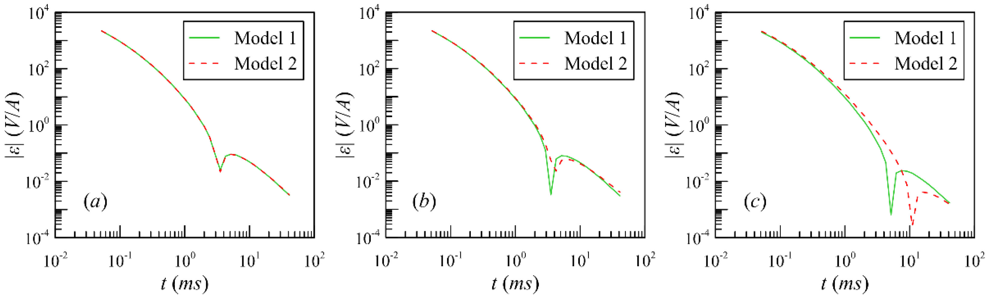
2.2. Singularity of IP-Affected TEM Data Inversion

The singularity of the TEM-IP joint inversion has been discovered in previous studies [39,40]. It is suggested that the singularity, which means that different models can produce identical responses, can be attributed to the complex responses and more unknowns. In consequence, the inversion quality greatly depend on the selection of initial model. Here we illustrate the singularity problem with a numerical example.

The model has three layers, and the parameters of each layer are shown in

Table 2. Parameters of the three-layer model (Model 1).

Parameters	h (m)	ρ (Ω·m)	m	c	τ (s)
Layer 1	100	400	0.06	0.55	10−2
Layer 2	50	100	0.06	0.55	10−2
Layer 3	-	800	0.60	0.55	10−2

. The observation parameters are: the central loop configuration is adopted, the length of the sides of the square transmitting loop is 100 m, the z-component attenuation voltage ε is recorded, the ramp length is 500 μs, and the transmitting current is 16 A. The responses are shown in Figure 3a with green line. An equivalent model can be easily found by data fitting, and its responses are shown in Figure 3a with red dash line. It can be seen that the parameters of the two models are significantly different, while the responses are almost exactly the same, with a small relative deviation of 0.21%. It is also worth mentioning that if the data fitting is performed with different starting points, a different equivalent model will be obtained. This explains the dependence on initial model and the non-uniqueness in the inversion. In order to recover reasonable layer parameters effectively using TEM-IP joint inversion, the singularity problem must be handled properly first. For the purpose of convenience, the model in Table 2 is named Model 1, and the equivalent model in

Table 3. Parameters of the equivalent three-layer model (Model 2).

Parameters	h (m)	ρ (Ω·m)	m	c	τ (s)
Layer 1	100	517	0.70	0.06	3.96 × 10−3
Layer 2	50	195	0.66	0.36	3.98 × 10−3
Layer 3	-	251	0.26	0.26	3.26 × 10−3

is named Model 2.

Kozhevnikov and Antonov have proved that the normally TEM currents and the IP currents have different patterns depending on loop configuration, and the IP effects in TEM data vary by different transmitting loop sizes [39,40]. Analogously, the IP effects in TEM data also vary with the changing of offset between the transmitter and the receiver. Figure 3b,c show the responses of Model 1 and Model 2 with an offset of 80 m and 120 m, respectively. We can see that the difference between the responses of Model 1 and Model 2 increases as the offset changes. It indicates that the TEM responses with different offsets can provide additional valid constraints for the inversion and weaken its singularity.

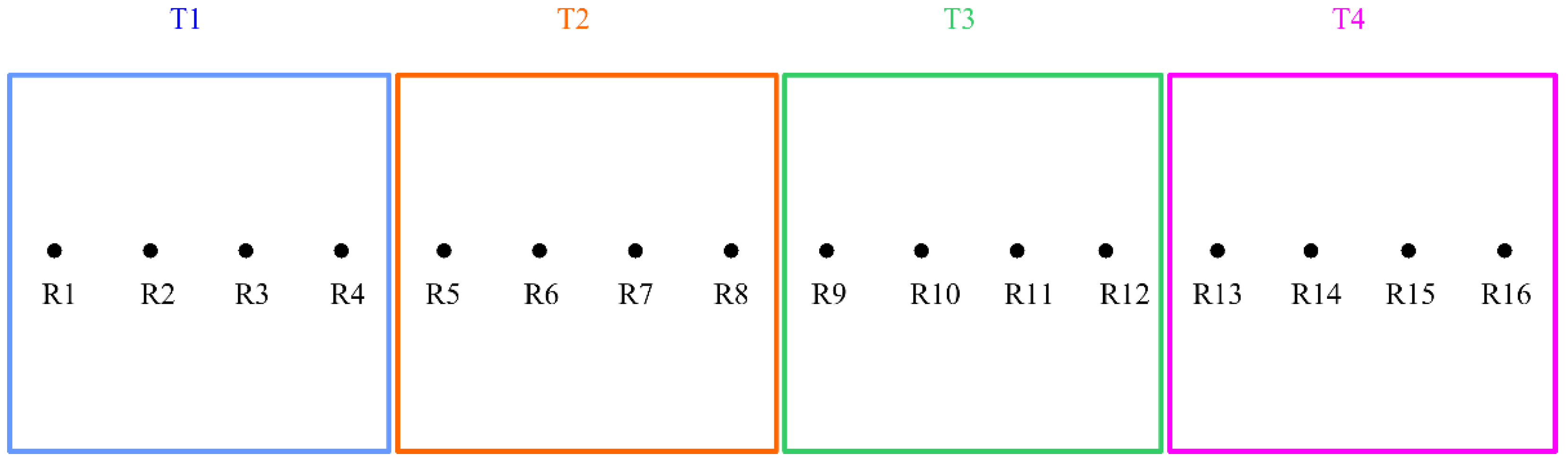
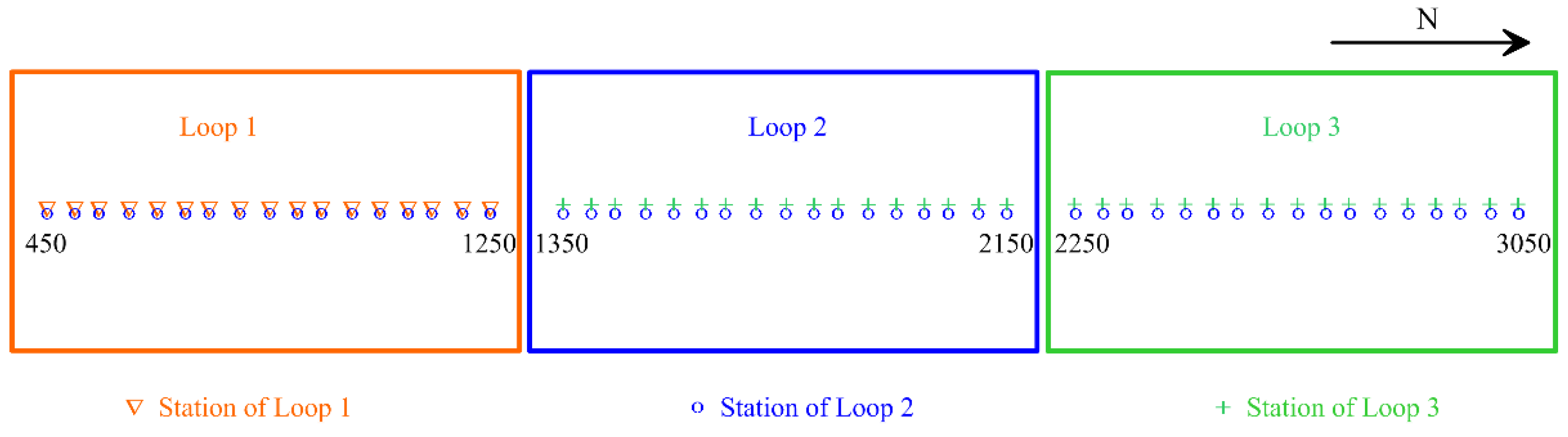
2.3. TEM Data Acquisition Using Dual Source

In the actual TEM exploration, a survey line is usually measured by a transmitting loop. One loop governs one or several stations on the survey line and moves forward after the measurement of one or several stations are completed. An example is shown in Figure 4, there are 16 stations on the survey line, and the fixed-loop configuration is adopted. Conventionally, the loop is placed at position T1 first, and the stations R1~R4 are measured. After that, the loop is moved to position T2, and the stations R5~R8 are measured. Other stations are measured successively until the survey line is completed. The alternative scheme using dual source is a modification of the conventional scheme. When the loop is moved to the next position, the stations governed by the last loop are measured again. Concretely, when the loop is moved to position T2, we measure the stations R1~R8, and when the loop is moved to position T3, we measure the stations R5~R12, and so forth. The modification guarantees every station to be measured twice with different offsets.

2.4. Joint Inversion of Dual-Source TEM Responses

The two datasets obtained by the TEM data acquisition scheme using dual source at each station can be combined for the joint inversion. For the purpose of fitting the TEM data over a wide dynamic range and suppressing the normally distributed noise, a least squares objective function is constructed based on the relative difference between the observed data and fitting data:

$$\phi =r^T{C}_{m}r+m^{T}Dm , r=\frac{d^{obs}-d^{fit}}{\left|d^{obs}\right|} , d=\left(\begin{array}{c}{d}_1\\ d_2\end{array}\right)$$

(9)

where d represents the TEM responses, the superscript ‘obs’ and ‘fit’ represent the observation and modeling responses, respectively, the subscript ‘1’ indicates that the dataset is acquired with the first offset, and the subscript ‘2’ indicates that the dataset is acquired with another offset, C_m is the weight matrix, m is the model parameter vector, D is the regularization matrix; generally, a smoothness or roughness matrix is adopted to improve the ill condition of the inversion problem. The particle swarm optimization is adopted for global optimization of the objective function (9) to recover the geoelectrical parameters.

3. Results

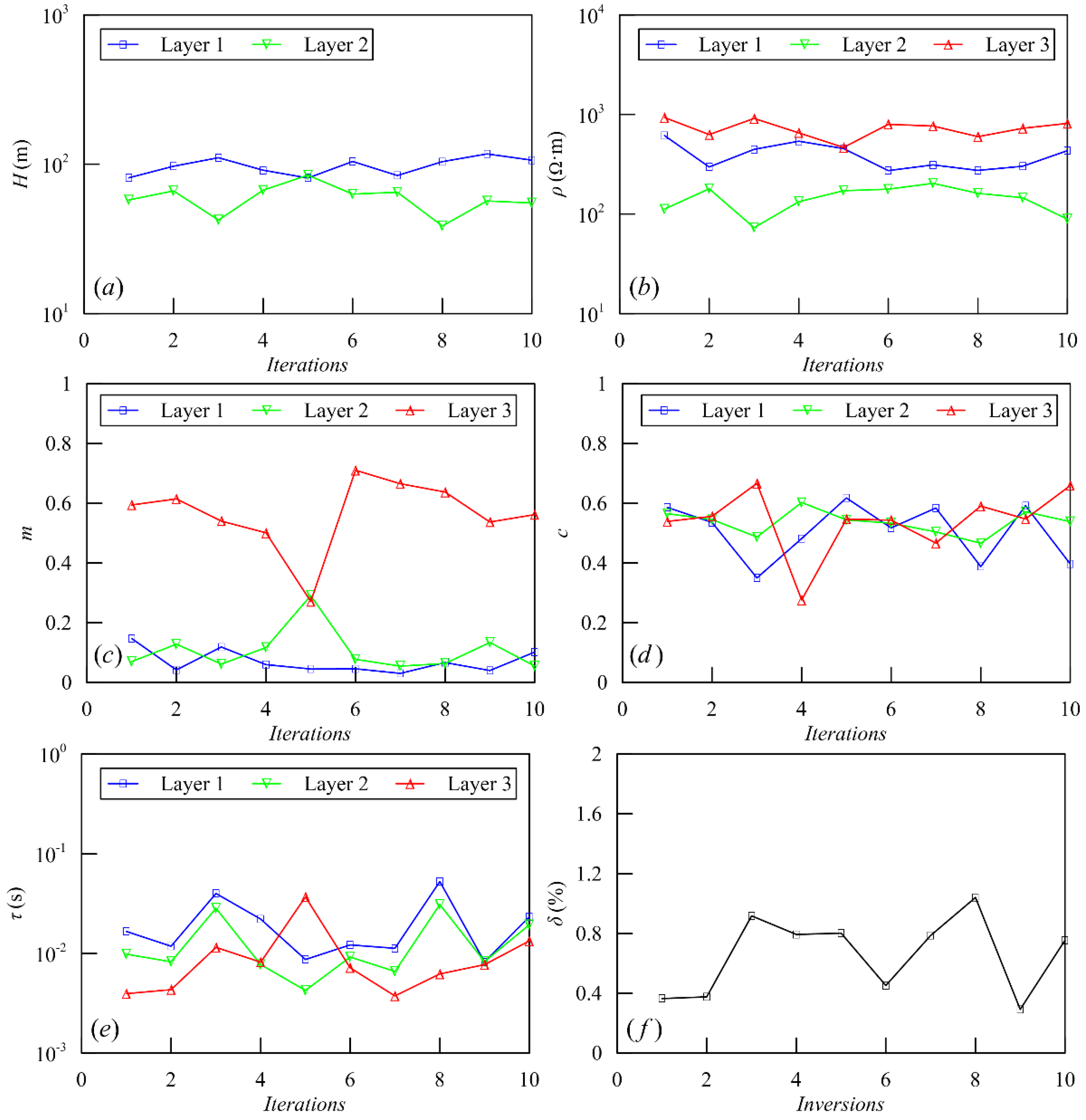
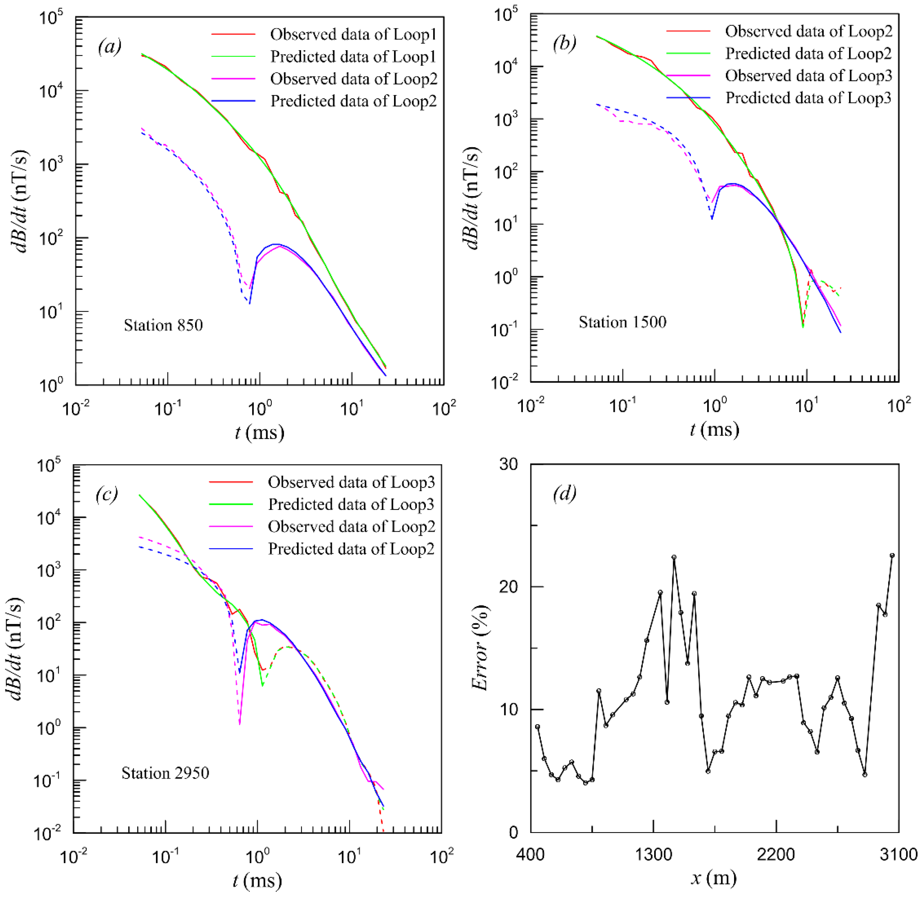
3.1. Synthetic Data Test

A numerical experiment is carried out to test the effect of the TEM data acquisition scheme using a dual source. A three-layer model (named Model 3) is designed, and the electrical parameters of each layer are shown in

Table 4. Parameters of the three-layer model (Model 3).

Parameters	h (m)	ρ (Ω·m)	m	c	τ (s)
Layer 1	100	800	0.05	0.55	10−3
Layer 2	50	100	0.30	0.55	10−3
Layer 3	-	800	0.05	0.55	10−3

. The transmitting loop size is 100 m × 100 m, the ramp length is 500 μs, and the transmitting current is set to 16 A. Preliminarily, the TEM responses are acquired using a central-loop configuration. The measuring station is located in (50 m, 50 m, 0 m). The transmitting loop is placed where its center coincides with the measuring station (zero offset). In order to evaluate the inversion quality, inversion of the single TEM dataset using central-loop configuration is conducted.

The PSO algorithm involves random search and is endowed with inherent randomness. The single dataset is an insufficient constraint for the inversion possibly, which would result in significantly different inversion models with good fitting. The inversion is conducted repeatedly for ten times, and the inversion parameters of each layer are plotted in Figure 5a–e, and the relative data fit errors of each inversion are shown in Figure 5f. The relative data fit errors are calculated as:

$$\delta =\sqrt{\frac{r^{T}r}{N-1}}\times 100\% , r=\frac{d^{obs}-d^{fit}}{\left|d^{obs}\right|} , d=\left(\begin{array}{c}{d}_1\\ d_2\end{array}\right)$$

(10)

where d represents the TEM responses, the superscript ‘obs’ and ‘fit’ represent the observation and modeling responses respectively, the subscript ‘1’ indicates that the dataset is acquired with the first offset, and the subscript ‘2’ indicates that the dataset is acquired with another offset, N is the number of elements in vector d. We can see that the true solution can be obtained occasionally, while the parameters of each inversion fluctuate greatly with a stable small fitting error. It indicates that all the ten inversion models are algebraic approximate solutions of the inversion problem, actually proves the singularity of inversion using the single central-loop dataset.

The dual-source TEM responses are acquired by an additional transmitting loop. It has the same geometry as the first loop except for its central location in (200 m, 50 m, 0 m). As a result, the datasets with the offset of zero and 150 m are both obtained. Then the joint inversion of the two datasets is also conducted repeatedly for ten times, and the inversion parameters of each layer are plotted in Figure 6. It is easily found that the parameters of each inversion are obviously stabilized and converge to the designed value. The convergence indicates that the TEM datasets using dual sources can provide effective constraints for the TEM-IP joint inversion problems.

It is worth noting that the fit errors of single-loop data are slightly larger than the ones of dual-loop data. This can be due to the more adequate constraints possibly. Inversion using single-loop data only fits one of the two datasets with different offsets, has fewer constraints and is easy to achieve a small fitting error, and the inversion combining the dual loop fits both the two datasets at the same time, the fitting error is the compound of the two datasets, which is more complex and not easy to decline iteratively, so it is slightly larger. However, the inversion combining the dual loop has more sufficient constraints on the inversion model, and the inversion parameters are more accurate.

The PSO takes longer to compute than traditional linear inversion methods. In our previous paper [38], the PSO was compared with the Gauss–Newton method, which is widely used in the inversion of geophysics data. After 50 iterations, the Gauss–Newton method took 1.6 min, while the PSO took 23 min. It indicates that the time cost of PSO may be 10 times more than that of the traditional quasilinear inversion algorithm. This can mainly be due to the large number of particles that require forward modeling in each iteration to ensure its global optimization capability. The results also show that although PSO requires more inversion time, the inversion converges to a small fitting error after 50 iterations, while the Gauss–Newton algorithm falls into a local minimum after 15 iterations with a large fitting error. Therefore, the time cost is worthwhile. Meanwhile, the PSO has the ability to learn and record the good solutions, and this guarantees its time cost to be much less than the complete Monte Carlo method and acceptable.

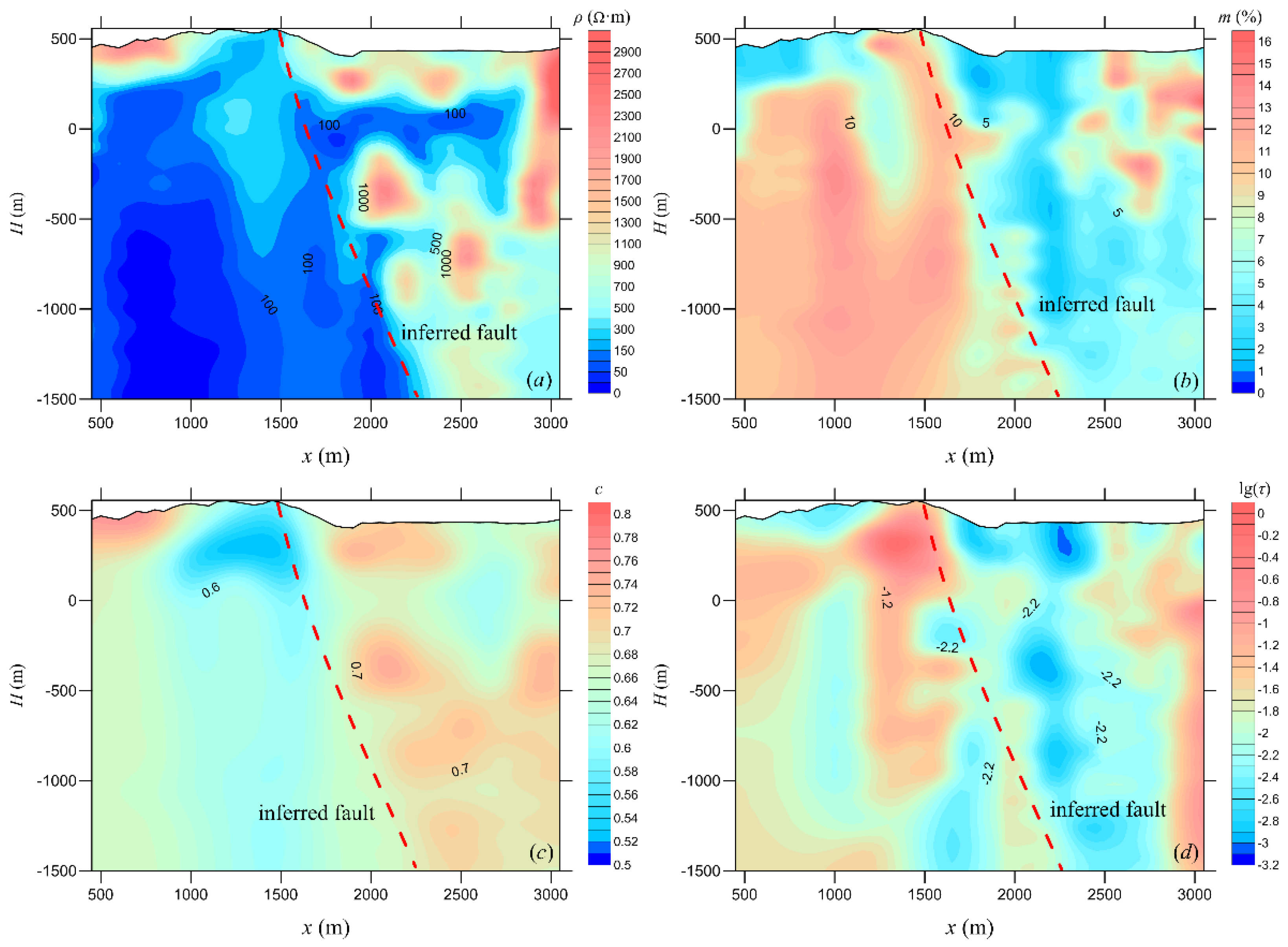
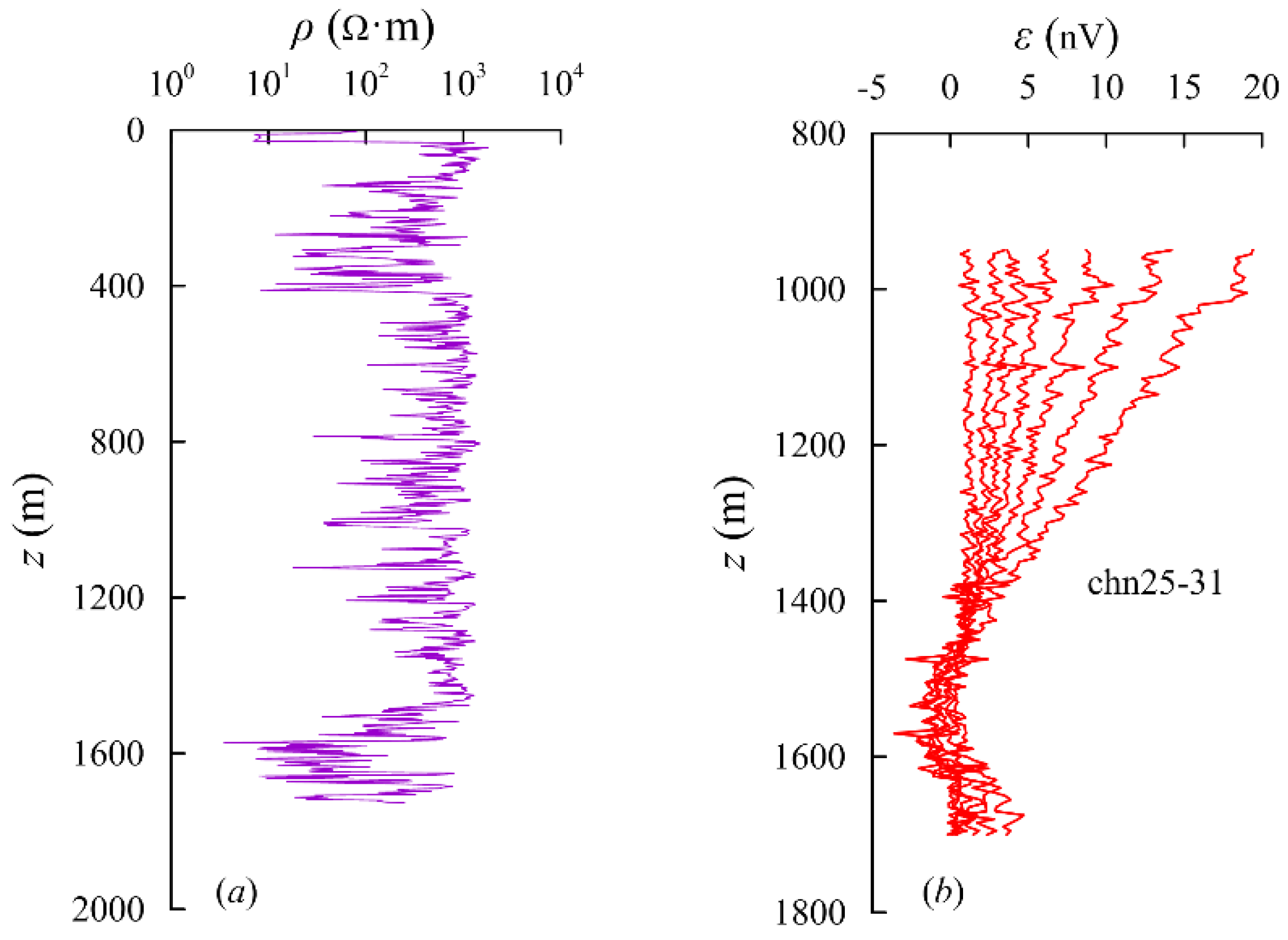
3.2. A Field Example: Baiyun Gold Deposit

The Baiyun gold deposit is one of the largest ore deposits in the Qingchengzi ore concentrated area, eastern Liaoning. The local strata in the Baiyun area are mainly composed of the third member of the Dashiqiao Formation and Gaixian Formation. The third member of the Dashiqiao Formation has a low resistivity commonly, which is mainly caused by the diopside diorite schist and graphite bearing marble. The Galaxian Formation is mainly composed of schist and granulite, which have middle to high resistivity. The strata have high chargeability due to the wide presence of graphite and pyrite [42]. In order to evaluate its deep metallogenic potential, the TEM survey was applied to the exploration of its strata and structures.

The TEM survey line consists of three 400 m × 900 m transmitting loops, and the vertical component of the dB/dt response is measured with a station spacing of 50 m. In consideration of the polarizable formation, the dual-source TEM geometry is adopted. Figure 7 shows the corresponding relationship between the transmitting loops and measuring stations using it.

Table 5. Parameters of field data collection.

Terms	Parameters	Terms	Parameters
Instrument	SMARTem24	Receiver type	Crone probe
Current	23 A	Receiver area	3850 m2
Time Base	50 ms	Stack times	512
Ramp time	122 μs	Receive signal	dBz/dt

shows the acquisition parameters. Finally, each station was measured twice with different loops, and we obtained 102 TEM datasets at 51 stations.

The joint inversion of dual-source TEM responses is conducted to fit the observation datasets and recover the electrical parameters of the formation. The initial model is not essential for the PSO algorithm, while the number of layers of the inversion model must be provided to determine the number of unknown variables. An eight-layer model which leads to 39 model parameters was employed for this example. For the stability of the inversion, a 1-order smooth regularization matrix was applied to ρ, m, c, and τ, respectively. In order to improve horizontal continuity, the inversion model of every station was set to a member of the initial particle swarm of the next station.

Data-fitting curves of several stations are shown in Figure 8a–c, where the dotted lines represent the negative TEM responses, and the fitting error of each measuring station is shown in Figure 8d. According to Figure 8, we can see that there is a good agreement between the observed and predicted data. The average fitting error of all stations is 10.66%, which indicates that the PSO inversion method is applicable in fitting dual-source TEM data.

Figure 9a–d shows the inversion cross-sections of ρ, m, c, and τ, respectively. For the purpose of validating the inversion results, the resistivity logging and TEM logging data from a drill hole located 100 m west of station 2000 were collected and shown in Figure 10a and Figure 10b, respectively. The sign reversals of TEM logging curves below 1400 m indicate that the formation has a high chargeability. Figure 9 and Figure 10 show that the inversion results agree well with the logging results on the parameters of resistivity and chargeability. A large fault extending deeper than 2000 m can be inferred according to the inversion resistivity and chargeability profiles. The fracture is characterized by low resistivity, high chargeability, low c, and large τ, which indicates the existence of pyritization and graphitization and implies the gold mineralization in depth.

4. Discussion and Conclusions

The forward modeling of IP-affected TEM responses using the Cole–Cole model and a frequency-time domain transformation was conducted and validated by Lee’s analytical solutions. A three-layer equivalent model pair illustrated the singularity of TEM-IP joint inversion clearly. The further simulation indicated that the joint of TEM responses with different offsets could provide additional constraints for the inversion and weaken its singularity.

The dual-source TEM data acquisition scheme was proposed based on forwarding modeling and analysis. The scheme modifies the conventional scheme to guarantee all stations to be measured twice with different offsets. The modification is slight and avoids a significant increase in the field work.

The global joint inversion method was established to handle non-monotonicity and singularity simultaneously. The objective inversion function was constructed by combining the relative error of dual-source TEM responses. The PSO algorithm was adopted to achieve global convergence.

The synthetic data test illustrated that the joint of the dual-source method greatly weakened the singularity and stabilized the inversion. The comparison showed the designed model parameters could be recovered with a much higher probability than the conventional single source inversion.

We applied the dual-source scheme and joint inversion method in this paper to actual data collected from the Baiyun gold mine. The inversion results were validated by resistivity logging and TEM logging results and showed well coincidence. The combining of the four parameters (ρ, m, c, and τ) revealed a large fault and predicted the gold mineralization below 2000 m.

References

1. Nabighian, M.N.; Macnae, J.C. Time Domain Electromagnetic Prospecting Methods. In Electromagnetic Methods in Applied Geophysics: Volume 2, Application, Parts A and B; SEG: Tulsa, OK, USA, 1991; pp. 427–520. [Google Scholar]
2. Asten, M.W.; Duncan, A.C. The quantitative advantages of using B-field sensors in time-domain EM measurement for mineral exploration and unexploded ordnance search. Geophysics 2012, 77, WB137–WB148. [Google Scholar] [CrossRef]
3. Yang, D.K.; Oldenburg, D.W. Three-dimensional inversion of airborne time-domain electromagnetic data with applications to a porphyry deposit. Geophysics 2012, 77, B23–B34. [Google Scholar] [CrossRef]
4. Chen, W.; Xue, G.Q.; Zhou, N.N.; Tang, D.M.; Hou, D.Y.; He, Y.M.; Lei, K.X.; Chen, K.; Li, H. Delineating ore-forming rock using a frequency domain controlled-source electromagnetic method. Ore Geol. Rev. 2019, 115, 103167. [Google Scholar] [CrossRef]
5. Di, Q.Y.; Zhu, R.X.; Xue, G.Q.; Yin, C.C.; Li, X. New development of the Electromagnetic (EM) methods for deep exploration. Chin. J. Geophys. 2019, 62, 2128–2138. [Google Scholar] [CrossRef]
6. Di, Q.Y.; Xue, G.Q.; Yin, C.C.; Li, X. New methods of controlled-source electromagnetic detection in China. Sci. China Earth Sci. 2020, 63, 1268–1277. [Google Scholar] [CrossRef]
7. Guo, Z.W.; Xue, G.Q.; Liu, J.X.; Wu, X. Electromagnetic methods for mineral exploration in China: A review. Ore Geol. Rev. 2020, 118, 103357. [Google Scholar] [CrossRef]
8. Li, R.H.; Hu, X.Y.; Xu, D.; Liu, Y.; Yu, N. Characterizing the 3D hydrogeological structure of a debris landslide using the transient electromagnetic method. J. Appl. Geophys. 2020, 175, 103991. [Google Scholar] [CrossRef]
9. Lee, T.J.; Thomas, L. A Review of the Application of Analytical Methods to the Prediction of Transient Electromagnetic Field Responses. Explor. Geophys. 1988, 19, 423–434. [Google Scholar] [CrossRef]
10. Swidinsky, A.; Hölz, S.; Jegen, M. On mapping seafloor mineral deposits with central loop transient electromagnetics. Geophysics 2012, 77, E171–E184. [Google Scholar] [CrossRef] [Green Version]
11. Raiche, A.P. Comparison of apparent resistivity functions for transient electromagnetic methods. Geophysics 1983, 48, 787–789. [Google Scholar] [CrossRef]
12. Zhang, Y.Y.; Li, X.; Yao, W.H.; Zhi, Q.Q.; Li, J. Multi-component full field apparent resistivity definition of multi-source ground-airborne transient electromagnetic method with galvanic sources. Chin. J. Geophys. 2015, 58, 2745–2758. [Google Scholar] [CrossRef]
13. Spies, B.R.; Eggers, D.E. The use and misuse of apparent resistivity in electromagnetic methods. Geophysics 1986, 51, 1462–1471. [Google Scholar] [CrossRef]
14. Xue, G.Q.; Li, H.; He, Y.M.; Xue, J.J.; Wu, X. Development of the Inversion Method for Transient Electromagnetic Data. IEEE Access 2020, 8, 146172–146181. [Google Scholar] [CrossRef]
15. Xue, G.Q.; Zhang, L.B.; Zhou, N.N.; Chen, W.Y. Developments measurements of TEM sounding in China. Geol. J. 2020, 55, 1636–1643. [Google Scholar] [CrossRef]
16. Christensen, N.B. Fast approximate 1D modelling and inversion of transient electromagnetic data. Geophys. Prospect. 2016, 64, 1620–1631. [Google Scholar] [CrossRef]
17. Lu, X.S.; Farquharson, C.; Miehé, J.M.; Harrison, G.; Ledru, P. Computer modeling of electromagnetic data for mineral exploration: Application to uranium exploration in the Athabasca Basin. Lead. Edge 2021, 40, 139a1–139a10. [Google Scholar] [CrossRef]
18. Engebretsen, K.W.; Zhang, B.; Fiandaca, G.; Madsen, L.M.; Auken, E.; Christiansen, A.V. Accelerated 2.5-D inversion of airborne transient electromagnetic data using reduced 3-D meshing. Geophys. J. Int. 2022, 230, 643–653. [Google Scholar] [CrossRef]
19. Cole, K.S.; Cole, R.H. Dispersion and Absorption in Dielectrics I. Alternating Current Characteristics. J. Chem. Phys. 1941, 9, 341–351. [Google Scholar] [CrossRef] [Green Version]
20. Pelton, W.H.; Ward, S.H.; Hallof, P.G.; Sill, W.R.; Nelson, P.H. Mineral discrimination and removal of inductive coupling with multifrequency IP. Geophysics 1978, 43, 588–609. [Google Scholar] [CrossRef]
21. Merriam, J.B. Induced polarization and surface electrochemistry. Geophysics 2007, 72, F157–F166. [Google Scholar] [CrossRef]
22. Gurin, G.; Titov, K.; Ilyin, Y.; Tarasov, A. Induced polarization of disseminated electronically conductive minerals: A semi-empirical model. Geophys. J. Int. 2015, 200, 1555–1565. [Google Scholar] [CrossRef] [Green Version]
23. Zhdanov, M.; Endo, M.; Cox, L.; Sunwall, D. Effective-Medium Inversion of Induced Polarization Data for Mineral Exploration and Mineral Discrimination: Case Study for the Copper Deposit in Mongolia. Minerals 2018, 8, 68. [Google Scholar] [CrossRef] [Green Version]
24. Li, H.; Xue, G.Q.; He, Y.M. Decoupling induced polarization effect from time domain electromagnetic data in a Bayesian framework. Geophysics 2019, 84, A59–A63. [Google Scholar] [CrossRef]
25. Zhou, N.N.; Lei, K.X.; Xue, G.Q.; Chen, W. Induced polarization effect on grounded-wire transient electromagnetic data from transverse electric and magnetic fields. Geophysics 2020, 85, E111–E120. [Google Scholar] [CrossRef]
26. Raiche, A.P. Negative transient voltage and magnetic field responses for a half-space with a Cole-Cole impedance. Geophysics 1983, 48, 790–791. [Google Scholar] [CrossRef]
27. Spies, B.R. A field occurrence of sign reversals with the transient electromagnetic method. Geophys. Prospect. 1980, 28, 620–632. [Google Scholar] [CrossRef]
28. Raiche, A.P.; Bennett, L.A.; Clark, P.J.; Smith, R.J. The use of Cole–Cole impedances to interpret the TEM response of layered earths. Explor. Geophys. 1985, 16, 271–273. [Google Scholar] [CrossRef]
29. Smith, R.S.; West, G.F. Inductive interaction between polarizable conductors: An explanation of a negative coincident-loop transient electromagnetic response. Geophysics 1988, 53, 677–690. [Google Scholar] [CrossRef]
30. Flis, M.F.; Newman, G.A.; Hohmann, G.W. Induced-polarization effects in time-domain electromagnetic measurements. Geophysics 1989, 54, 514–523. [Google Scholar] [CrossRef] [Green Version]
31. Lee, T. Transient electromagnetic response of a polarizable ground. Geophysics 1981, 46, 1037–1041. [Google Scholar] [CrossRef]
32. Knight, J.H.; Raiche, A.P. Transient electromagnetic calculations using the Gaver-Stehfest inverse Laplace transform method. Geophysics 1982, 47, 47–50. [Google Scholar] [CrossRef]
33. Yin, C.C.; Liu, B. The research on the 3D TDEM modeling and IP effect. Chin. J. Geophys. 1994, 37, 486–492. [Google Scholar]
34. Marchant, D.; Haber, E.; Oldenburg, D.W. Three-dimensional modeling of IP effects in time-domain electromagnetic data. Geophysics 2014, 79, E303–E314. [Google Scholar] [CrossRef]
35. Smith, R.S.; Klein, J. A special circumstance of airborne induced-polarization measurements. Geophysics 1996, 61, 66–73. [Google Scholar] [CrossRef]
36. Yu, C.T.; Liu, H.F.; Zhang, X.J.; Yang, D.Y.; Li, Z.H. The analysis on IP signals in TEM response based on SVD. Appl. Geophys. 2013, 10, 79–87. [Google Scholar] [CrossRef]
37. Flores, C.; Peralta-Ortega, S.A. Induced polarization with in-loop transient electromagnetic soundings: A case study of mineral discrimination at El Arco porphyry copper, Mexico. J. Appl. Geophys. 2009, 68, 423–436. [Google Scholar] [CrossRef]
38. Zhi, Q.Q.; Deng, X.H.; Wu, J.J.; Li, X.; Wang, X.C.; Yang, Y.; Zhang, J. Inversion of IP-Affected TEM Responses and Its Application in High Polarization Area. J. Earth Sci. 2021, 32, 42–50. [Google Scholar] [CrossRef]
39. Kozhevnikov, N.O.; Antonov, E.Y. Joint inversion of IP-affected TEM data. Russ. Geol. Geophys. 2009, 50, 136–142. [Google Scholar] [CrossRef]
40. Kozhevnikov, N.O.; Antonov, E.Y. Inversion of IP-affected TEM responses of a two-layer earth. Russ. Geol. Geophys. 2010, 51, 708–718. [Google Scholar] [CrossRef]
41. Key, K. 1D inversion of multicomponent, multifrequency marine CSEM data: Methodology and synthetic studies for resolving thin resistive layers. Geophysics 2009, 74, F9–F20. [Google Scholar] [CrossRef]
42. Wu, J.J.; Zhi, Q.Q.; Deng, X.H.; Wang, X.C.; Yang, Y.; Zhang, J.; Dai, P. Exploration of Deep Geological Structure of Baiyun Gold Deposit in Eastern Liaoning Province with TEM. Earth Sci. 2020, 45, 4027–4037. [Google Scholar]
Figure 1. The 1D layered-earth model.
Minerals 12 00684 g001
Figure 2. Validation of the modeling results. (a) The Lornex model; (b) The Copper cities model; (c) The Kidd Creek model.
Minerals 12 00684 g002
Figure 3. The TEM respones of the equivalent three-layer models. (a) The Central loop; (b) Offset = 80 m; (c) Offset = 120 m.
Minerals 12 00684 g003
Figure 4. An example of TEM survey using the fixed-loop configuration.
Minerals 12 00684 g004
Figure 5. The inversion parameters of Model 3 using single source. (a) The layer thickness; (b) The resistivity; (c) The chargeability; (d) The frequency exponent; (e) The time constant; (f) The relative fitting error.
Minerals 12 00684 g005
Figure 6. The inversion parameters of Model 3 using dual source. (a) The layer thickness; (b) The resistivity; (c) The chargeability; (d) The frequency exponent; (e) The time constant; (f) The relative fitting error.
Minerals 12 00684 g006
Figure 7. Schematic diagram of transmitting loops and TEM stations.
Minerals 12 00684 g007
Figure 8. Fitting curves and fitting error of different stations. (a) Fitting curves of station 850; (b) Fitting curves of station 1500; (c) Fitting curves of station 2950; (d) Fitting errors of all stations.
Minerals 12 00684 g008
Figure 9. The inversion cross-sections. (a) The resistivity; (b) The chargeability; (c) The frequency exponent; (d) The time constant.
Minerals 12 00684 g009
Figure 10. The logging curves. (a) The resistivity logging curves; (b) The TEM logging curves of 25–31 channels.
Minerals 12 00684 g010