Article

Quantification of Small-Scale Heterogeneity at the Core–Mantle Boundary Using Sample Entropy of SKS and SPdKS Synthetic Waveforms

by
Surya Pachhai
1,*,
Michael S. Thorne
1,* and
Tarje Nissen-Meyer
2
1
Department of Geology and Geophysics, University of Utah, 115 S 1460 E #383, Salt Lake City, UT 84112, USA
2
Department of Earth Sciences, University of Oxford, South Parks Road, Oxford OX1 3AN, UK
*
Authors to whom correspondence should be addressed.
Minerals 2022, 12(7), 813; https://doi.org/10.3390/min12070813
Submission received: 2 May 2022 / Revised: 13 June 2022 / Accepted: 23 June 2022 / Published: 26 June 2022

Abstract

:
Qualitative and quantitative analysis of seismic waveforms sensitive to the core–mantle boundary (CMB) region reveal the presence of ultralow-velocity zones (ULVZs) that have a strong decrease in compressional (P) and shear (S) wave velocity, and an increase in density within thin structures. However, understanding their physical origin and relation to the other large-scale structures in the lowermost mantle are limited due to an incomplete mapping of ULVZs at the CMB. The SKS and SPdKS seismic waveforms is routinely used to infer ULVZ presence, but has thus far only been used in a limited epicentral distance range. As the SKS/SPdKS wavefield interacts with a ULVZ it generates additional seismic arrivals, thus increasing the complexity of the recorded wavefield. Here, we explore utilization of the multi-scale sample entropy method to search for ULVZ structures. We investigate the feasibility of this approach through analysis of synthetic seismograms computed for PREM, 1-, 2.5-, and 3-D ULVZs as well as heterogeneous structures with a strong increase in velocity in the lowermost mantle in 1- and 2.5-D. We find that the sample entropy technique may be useful across a wide range of epicentral distances from 100° to 130°. Such an analysis, when applied to real waveforms, could provide coverage of roughly 85% by surface area of the CMB.

1. Introduction

The core–mantle boundary (CMB) separates the heterogeneous solid mantle from the nearly homogeneous liquid outer core. The shear (S)-wave velocity, and density contrast at the CMB is the largest in the Earth’s interior and exceeds that of the Earth’s surface [1]. Additionally, a significant amount of heat flows from the core to the mantle creating a thermal boundary layer at the bottom of the mantle [2,3]. This unique setting hosts a wide variety of lower mantle phenomena and features, as depicted in Figure 1, including the following: core–mantle interaction, chemical segregation and phase transition of minerals, presumed remnants of subducted slabs, possible reservoirs of primordial material, formation of deep mantle plumes, and directional dependence (anisotropy) of material properties indicative of mantle flow [4]. The study of lateral variation of seismic properties near the CMB is crucial to improve our understanding of the ongoing processes and dynamics of the Earth’s interior and their link to the formation and evolution of the planet.
Seismological studies show heterogeneities in the lowermost mantle over a range of length scales. At the largest length scales, the lowermost mantle is dominated by continental sized low velocity features beneath Africa and Pacific [5,6,7,8,9,10]. These features are widely known as large-low shear velocity provinces (LLSVPs) as they were first consistently observed in S-wave velocity models. The LLSVPs are surrounded by higher velocity structures that are usually interpreted as relatively cold slab material [11,12,13,14]. The existence of these LLSVPs has generally been agreed upon between the various global S-wave tomography models, but there exist primary differences in the small-scale details within these structures [15]. More recently, P-wave tomographic inversions have also demonstrated large scale P-wave velocity reduction coincident with LLSVP locations [6,16]. Hence, in this paper, we refer to all such regions as large low-velocity provinces (LLVPs).
Seismic heterogeneities at the shortest and medium-length scale (on the order of 10 s to 100 s of km) are below the resolution limit of global tomographic approaches. However, with increased high-quality data and new measurement techniques, the ability to resolve structure in the lowermost mantle structure has significantly improved in the last two decades. As a result, shorter-length scale heterogeneities have been imaged [17,18,19,20]. One of the most prominent features that cannot be detected in seismic tomography are ultralow-velocity zones (ULVZs). Although an exact definition of what constitutes a ULVZ is currently lacking, these features are commonly described as being thin (typically less than 40 km) with strong decreases in S- (up to 50%) and P- (up to 25%) wave velocities, with an associated increase in density of up to 30% [21]. Size constraints on ULVZs are typically lacking, but they may span a wide variety of length scales from a few 10 s of km [22,23,24] up to several hundred km [25,26,27]. Although ULVZ structures are small, the study of their physical origin is likely essential for understanding the chemical and dynamical processes in the lowermost mantle, and their link to large-scale mantle structures [28,29]. However, most of the CMB region remains unexamined in terms of ULVZs, and their interpretation is generally based on ULVZs found in limited locations.
ULVZs were first detected using the SPdKS seismic phase (Figure 1). SPdKS is a seismic phase similar to the SKS arrival but contains additional legs of P-wave diffraction along the mantle side of the CMB [30,31]. After the initial discovery of ULVZs using SPdKS, a wide variety of seismic probes have been used to image ULVZ structure. For example, pre- and post-cursors of core-reflected arrivals such as (1) PcP—a P-wave reflected from the CMB [32,33], (2) ScP—a S-wave converted to P and reflected back from the CMB as P [34,35], (3) ScS—a S-wave reflected from the CMB [27,36], (4) pre-cursors to the core-refracted arrival PKP—a P-wave passing through the outer core [22,37,38], (5) post-cursors to SKS—a S wave passing through the outer core as P [39], (6) post-cursors to the core-diffracted Sdiff arrival—a S wave diffracted along the mantle side of the CMB [40,41], (7) slowness deviations to the core-diffracted Pdiff arrival—a P wave diffracted along the mantle side of the CMB [42], and (8) slowness deviations to CMB diffractions of the core-refracted P-arrival PKKPdiff [43]. Nonetheless, ULVZ locations and their properties seem to depend on the type of data analyzed due to their differing sensitivity and resolving power. For example, Thorne and Garnero [44] infer ULVZs in a wide region near the west Pacific using SPdKS waveforms, but Idehara, Yamada and Zhao [23] only found ULVZs in a subset of this region using higher frequency ScP and PcP waveforms. Similarly, Cottaar and Romanowicz [25] indicated the presence of a large ULVZ beneath the central Pacific using long-period Sdiff waveforms, where Luo et al. [45] did not find ULVZ evidence using higher frequency PKP waveforms. Additionally, Vidale and Hedlin [46] inferred ULVZs beneath the Southwest Pacific from the presence of strong PKP pre-cursor arrivals, whereas Garnero and Vidale [34] did not find ULVZs in this location using ScP waveforms. These examples illustrate that ULVZ locations are still poorly resolved and that different types of data used have different sensitivity to the underlying structures.
In addition to the ULVZ locations, ULVZ parameters (thickness, velocity, density, and shape) are also poorly understood due to non-uniqueness resulting from trade-offs between ULVZ parameters [47,48]. Traditionally, ULVZ parameters are estimated by forward waveform modeling of core-reflected and core-diffracted waveforms [25,49,50,51]. In this approach, ULVZ thickness and velocity reductions are approximated based on the observation of pre- and post-cursors. Then, waveforms are simulated for 10 s to 1000 s of ULVZ models to find a model that best explains the observed features. However, identification of these additional pre- and post-cursors due to ULVZs is challenging, particularly when pre- and post-cursors are weak, and the wavefield interferes constructively and/or destructively, resulting in unexpected features in the waveforms. This may be the reason that forward waveform modeling of, for example, long-period SPdKS waveforms show poor fit with those observed at longer epicentral distances, although most of the SKS signal at shorter epicentral distances fits well [51,52]. Such a poor fit may also be due to the long-period noise present in the data and/or 3-D wave front healing effects not present in the modeling. Fully non-linear Bayesian waveform inversion would be the best alternative method that provides rigorous parameter values and their uncertainties by balancing the trade-off between misfit and model complexity [24,48,53]. However, Bayesian inversion has not yet been computationally feasible for 2-D and 3-D modeling of ULVZs.
Many previous studies have interpreted ULVZs as a partial melt of the lowermost mantle material [54,55] based on a 3:1 ratio of S- to P-wave velocity perturbations. This partial melt explanation is attractive in light of a possible correlation between ULVZ locations and the surface locations of hotspot volcanism [56]. This interpretation becomes challenging for ULVZs that are detected at high-velocity regions of the lowermost mantle [52,57,58,59], where temperatures are assumed to be far lower than that in the LLSVPs, yet partial melting of mid-ocean ridge basalt (MORB) material in downwelling slabs may account for such observations [60]. Other mechanisms such as the existence of iron-rich ferropericlase, (Mg,Fe)O, can also explain an increase in density and a decrease in velocity [61,62] as well as to contribute to the observed lower mantle anisotropy [63,64]. It has also been argued that iron-enriched post-perovskite can explain such features [65]. Yet, it is unclear whether post-perovskite is stable at the lowermost mantle pressure and temperature conditions. Other studies suggest that ULVZs can be due to products of chemical reaction between the silicate mantle and Fe-rich core [66,67] which could also create a thin core–mantle transition zone (CMTZ) [68], slab-derived materials [69,70], and the remnants of Earth’s early differentiation [53,71]. Evidence has also been put forth that light sediments accumulating under the CMB, called core-rigidity zones (CRZs) may also account for some of the seismic observations [66,72]. Thus, the physical origin of ULVZs is still unknown, and a single mechanism may not explain all the observed ULVZs.
In summary, ULVZs are poorly known in terms of their location, their seismic properties and uncertainties, and consequently their physical origin. In order to better understand the physical cause of ULVZs and their possible link to the large-scale structure and dynamics, we need to investigate ULVZs in a wider region of the CMB. Previous studies have examined nearly 17% by surface area of the CMB out of which approximately 10% of the CMB locations contained ULVZs [21]. Recently, Thorne et al. [58,59] used a global dataset of SPdKS waveforms and analyzed a subset of these data in the distance range from 106° to 115° in search of highly anomalous SPdKS waveforms. This limited distance range sampled roughly 57% of the CMB area, and they identified several new possible ULVZ locations such as beneath North Africa, East Asia, and north of Papua New Guinea demonstrating that between 10 and 20% of the CMB area may contain ULVZs. These studies focused on finding evidence from some of the most pronounced SPdKS seismic waveform anomalies. Yet, these anomalies are not as readily identified in recordings at larger, or shorter, epicentral distances. Furthermore, ULVZs may be associated with more subtle waveform features that were not considered in those studies.
In this study we explore an alternate method to characterizing ULVZ existence that may have sensitivity at a wider epicentral distance range than utilized in Thorne et al. [58,59]. In this paper, we measure the waveforms complexity assuming that as the seismic waveform interacts with ULVZ structure, the ensuing scattering of seismic energy leads to a more irregular waveform. Here, we estimate waveform complexity by measuring the multi-scale sample entropy (MSE) of the time series [73,74]. The method is based on the sample entropy (SE) approach first introduced by Richman and Moorman (2000) but is computed at different decimating factors (defined as scale). For a fixed scale, waveforms with higher complexity produce a higher value of sample entropy, while signals with a higher degree of regularity (i.e., lower complexity) yield lower values of entropy. This approach has been regularly applied in health sciences to discriminate between states of health in individual. For example, measurements of irregularity in an individual’s heart beat could be an indicator of poor heart health [74,75,76,77]. However, variations of the SE approach have been applied in a wide variety of settings such as in analyzing climate data [78] and structural health monitoring of buildings [79]. To our knowledge, this approach has not yet been applied to seismic data to characterize waveform complexity.
In the case of seismic data, waveforms in the SKS/SPdKS time window display a decrease in the degree of regularity when the structures sampled by these arrivals deviates from the reference 1-D Earth model [1]. Therefore, the SE of waveforms that sense lower mantle structure have higher complexity due to responses that appear to be more scattered or less ordered than low complexity systems such as 1-D Earth model. In this paper, we assess the feasibility of the method by applying it to synthetic waveforms prepared for 1-D, 2.5-D, and 3-D ULVZ models as well as explore the possibility of using the approach to detect high and ultra-high velocity zones (UHVZs) [80]. Our synthetic experiments suggest that the SE increases with the strength and size of ULVZ structures in a systematic manner that could be used to detect ULVZs across a much wider range of epicentral distance than have been used in previous studies. In a follow-up paper, we then apply this approach to a global data-set of SKS/SPdKS waveforms [26,58,59].

2. The Sample Entropy Method
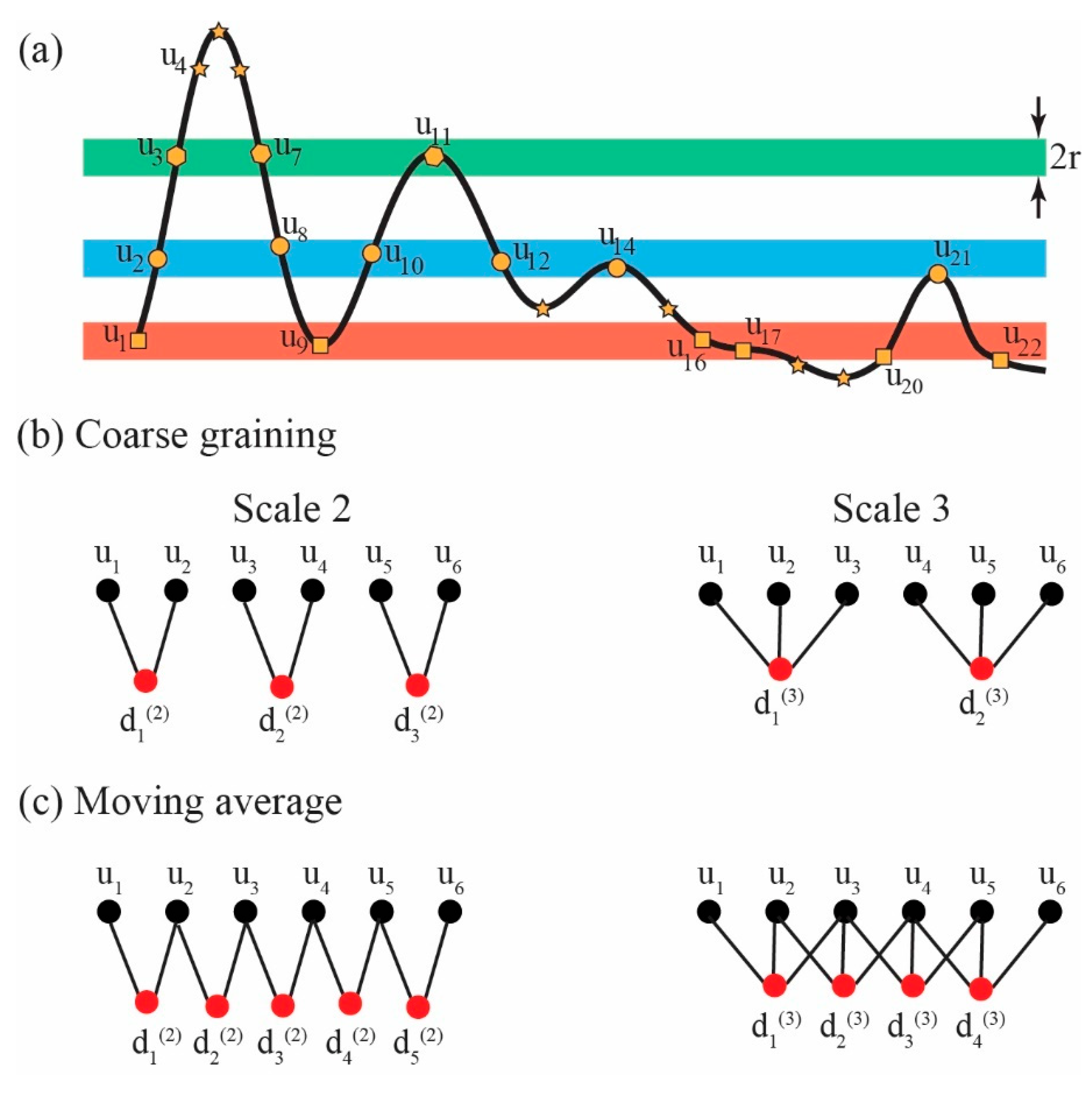
2.1. Sample Entropy

When seismic waves pass through structure that has a contrast in physical properties (either ULVZ or other features), the waveforms may display greater complexity due to conversions, reflections, and scattered waves. Here, we estimate the waveform complexity by measuring the sample entropy (SE). SE quantifies complexities based on the degree of similarity and randomness of data points within a given threshold. Statistically, it can be defined as the logarithmic ratio of the number of matches of a m consecutive data-point template to the number of matches of a m + 1 consecutive data-point template [75].
Figure 2 illustrates an example computation of SE for an SKS/SPdKS displacement time series with 22 points, u 1 , u 2 , u 3 , …, u 22 . In the example shown in Figure 2, we construct a m -point template (in this case, m = 2 with u 2 = u 1 , u 2 ). We then search for the number of m -point vector pairs in the trace that match within a specified threshold (r). The threshold is defined as a range in amplitudes centered on the sample points used in the template. For example, in Figure 2, we see that the two-point template u 1 , u 2 matches with u 9 , u 10 and u 20 , u 21 within the threshold. However, u 8 , u 9 is not a match as the sequence occurs in the opposite order. We count the total number of m -point vectors matching the template vector within the threshold which is N   m ,   r = 2 . The same procedure is repeated for the template with m + 1 dimension (i.e., in our example in Figure 3, u m + 1 = u 3 = u 1 , u 2 ,   u 3 ). The three-point template is matched only by the [ u 9 , u 10 ,   u 11 ] vector in our example. Therefore, the total number of m + 1 -point vector matches with an additional dimension is N   m + 1 , r = 1 . Then, the SE is estimated as a negative logarithm of the ratio of a total number of matches of 3-point template with that of 2-point template.
S E m , r = l n N m + 1 ,   r N m ,   r
In our example of Figure 2, we would obtain:
S E 2 , r = l n 1 2 = 0.6931
If we find more matches with the 2-point template, then the measured sample entropy would increase, indicating more variability or complexity in the signal. For example, if N m , r = 5     S E 2 , r = l n 1 5 = 1.6094. Finding more matches in the 3-point template, or less matches in the 2-point template, would result in a lowering of the SE measurement indicating less variability or complexity.

2.2. Multi-Scale Sample Entropy

Single point computation of sample entropy can be unreliable, as the statistical properties of the time series changes with the decimating factor, which is called the scale factor. Therefore, sample entropy is computed at various scales to provide reliable entropy estimates [76] and is known as multi-scale sample entropy (MSE). MSE works in two steps: in the first step, the time series is decimated by computing an average of non-overlapping consecutive points defined by scales ( τ ) (Figure 3b). This process is known as coarse-graining. For a given time series with n points u 1 , u 2 , u 3 , …, u n . The coarse-grained time series ( d ) at scale ( τ ) is obtained by,
d j τ = 1 τ i = j 1 τ + 1 j τ u i ,   with   1 j n / τ
The length of the coarse-grained time series is given by n / τ . For scale 1, coarse-grained and original time series have the same number of data points. The number of data points in the time series decreases by a factor of scale. Example coarse-graining at scales 2 and 3 is shown in Figure 2b.
Then, SE is estimated, in the second step, for each decimated time series as,
S E m , r , τ = l o g N m + 1 ,   r , τ N m ,   r , τ
This equation indicates that SE inherently depends on the number of data points (i.e., sampling interval), tolerance threshold ( r ), and scale (τ). To obtain robust statistics, a large number of data points are required. Therefore, when the time series to be analyzed becomes short, particularly for the analysis of single seismic phase within a limited time window, the number of points becomes significantly reduced at larger scales due to the coarse-graining. Therefore, MSE calculations becomes imprecise and sometimes the sample entropy becomes undefined due to two reasons: (1) when the number of points becomes too small, regularity becomes poor, and no matches appear (i.e., N   m   = 0, and N   m + 1   = 0), resulting in undefined entropy, and (2) the variance increases significantly when the matches are few. Several algorithms have been proposed to address this issue [77]. One approach is to use the moving average (Figure 2c) instead of coarse-graining (Figure 2b). This algorithm is often preferred for short time series when there are not many points for coarse-graining [81]. For a given time series with n points, the moving averaged time series is given by,
d j τ = 1 τ i = j j + τ 1 u i ,   with   1 j n τ + 1
The number of points for moving averaged time series becomes n τ + 1 . This means that the time series for scale 1 is the original signal. In contrast to the coarse-graining approach, the number of data points still remains higher.
Another, similar method that is employed when small sample sizes exist is called the composite multi-scale sample entropy (CMSE) technique [82,83]. For scale factor, τ, the CMSE is defined as:
CMSE m , r , τ = 1 τ j = 1 τ S E d j τ , m , r .

3. Synthetic Analysis of Sample Entropy

To demonstrate the feasibility of using entropy techniques on SKS/SPdKS waveforms and to determine which parameter values to use in the calculations, we tested the technique on a suite of synthetic seismograms computed for 1-, 2-, and 3-D models of both low- and high-velocity anomalies at the CMB.

3.1. Sample Entropy of 1-D Models

We computed seismograms for 1-D synthetic models using the full waveform reflectivity technique [84,85]. We considered various models to test the full range of expected low-velocity and ultra-low velocity parameters. For ULVZ models, we simulated SKS/SPdKS waveforms for the following parameters (1) S-wave velocity perturbation (δVS) varied from −50 to 0% in 5% increments (all percentages reported with respect to the PREM model [1]), (2) P-wave velocity perturbation (δVP) varied from −50 to 0% in 5% increments, (3) ULVZ height varied from 0 to 50 km in 5 km increments, (4) density perturbation (δρ) varied from −20% to +30% in 10% increments. In total, this gave us 3961 unique 1-D models. We also computed synthetics for an identical suite of high velocity and ultra-high velocity parameters, which only differed in that δVS varied from 0 to +50% in 5% increments and δVP varied from 0 to +50% in 5% increments. As a result, we have an additional 3961 high velocity models. All synthetics were computed for a 500 km source depth. We chose larger event depths to ensure that depth phases such as sSKS do not interfere with our measurements. UHVZ models are computed to S-wave velocity increases of up to 50% in symmetry with the ULVZ models; however, the largest reported S-wave velocity increases are on the order of +20%, which could be related to diamond-bearing structures [86].
Example synthetic seismograms at three epicentral distances (100°, 110°, and 120°) are shown in Figure 3a–c as a function of the strength of the ULVZ anomaly. We define ULVZ strength as the ULVZ thickness (h) multiplied by the sum of velocity perturbations. That is,
ULVZ   Strength = h × δ V S + δ V P ,
which is modified from the ULVZ strength parameter of Rondenay et al. (2010). Figure 3a–c shows that as ULVZ strength increases the apparent complexity of the seismic waveforms also increases and ultimately levels out at ULVZ strengths of roughly 2500 to 3000.
We present SE results in Figure 3d–f grouped into three epicentral distances of 100°, 110°, and 120°. These distances are chosen as representative of the different waveform behavior observed in previous studies [44,51]. (1) At a distance of around 100°, SPdKS is not yet generated, and only the SKS arrival exists in prediction from the PREM model. However, previous synthetic testing [51] has demonstrated that SKS pre- and post-cursors to SKS may be visible at distances from roughly 95° to 105°. These post-cursors may be related to converted phases at the ULVZ boundaries, while the pre-cursors are likely related to the conversion from S-to-P at the top of the ULVZ [52]. (2) Both synthetic testing and previous data analysis has shown that waveforms recorded at distances from roughly 106° to 115° show highly anomalous SPdKS recordings [51,52,58] and may also be the most diagnostic of ULVZ presence [44]. (3) At larger epicentral distances roughly greater than 115°, waveforms have been suggested to be less diagnostic of ULVZ presence and more similar to PREM [44].
To calculate the SE, we first preprocess the synthetic seismograms using the following steps: (1) we resample the seismograms onto a 0.1 s interval, (2) we cut the seismogram into a window starting 25 s before and 50 s after the PREM predicted SKS arrival, noting that we have 750 samples at the 0.1 s interval, (3) we normalize the maximum amplitude in the time window to unity, and (4) we differentiate the seismograms to velocity. We calculate SE on velocity seismograms in order to remove potential long-period signals that may be present in displacement seismograms. Here, we calculate the SE using a match length (m) = 2 and a threshold (r) = 0.2. SE measurements depend on all of the above parameters. We chose these specific values by systematically varying all parameters and checking which combination of parameters maximized the range of SE values measured from the 1-D synthetics. We observe that there is an overall increase in SE as a function of ULVZ strength (Figure 3d–f). The SE increases up to a strength of roughly 2500 to 3000, depending on epicentral distance, before leveling out. In this 1-D case, entropy levels out due to the fixed window in which we calculate entropy. At the largest ULVZ strengths, the SPdKS arrival is delayed beyond the chosen time window. In practice, we have not observed SPdKS arrivals beyond the chosen time window in real data so we keep the window fixed at this length. A ULVZ with δVS = −45% and δVP = −15% and a ULVZ strength of 2500 km·% would correspond to a 40 km-thick ULVZ. ULVZ strength values above the 2500 to 3000 range are likely in the most extreme range of ULVZ properties. However, some studies have suggested that ULVZs may exist at these large ULVZ strengths [87,88].
In evaluating this suite of ULVZ models we note that the measured SE has a mild correlation with increases in ULVZ thickness (h), S-wave velocity decrease (δVS), and P-wave velocity reduction (δVP). Yet, the ULVZ strength measurement shows the strongest pattern. This example illustrates that we may be directly assessing the ULVZ strength by measuring the SE. Although we may not directly be able to determine what the ULVZ parameters are from a measurement of SE, it may provide a means of identifying areas of the CMB that have the most anomalous heterogeneities.
For the high velocity and ultra-high velocity models there is almost no change in SE across the suite of 1-D models examined. Indeed, as the UHVZ strength increases (that is, larger thicknesses coupled with large S- and P-wave velocity increases), the SE actually decreases as the seismic waveforms appear simpler (Figure 4). Figure 4 shows a clear SPdKS arrival for the PREM model (at the bottom of the plot), but there is relatively little energy in addition to the SKS arrival for δVS = δVP = +50% (at the top of the plot). This is because as the seismic velocity is increased in the UHVZ the SPdKS phase is not generated due to the lack of critical ray parameter for S to Pdiff conversion at the CMB. Thus, the seismograms appear simpler. These experiments for 1-D models of ULVZs and UHVZs suggest that the SE is highly sensitive to ULVZs but has almost no sensitivity to UHVZs. This could also imply that for the SPdKS time window, observations of large-scale regions with an apparent decrease in SE could indicate UHVZ presence. This could be confirmed by subsequent analysis of the waveforms demonstrating a lack of SPdKS arrival.

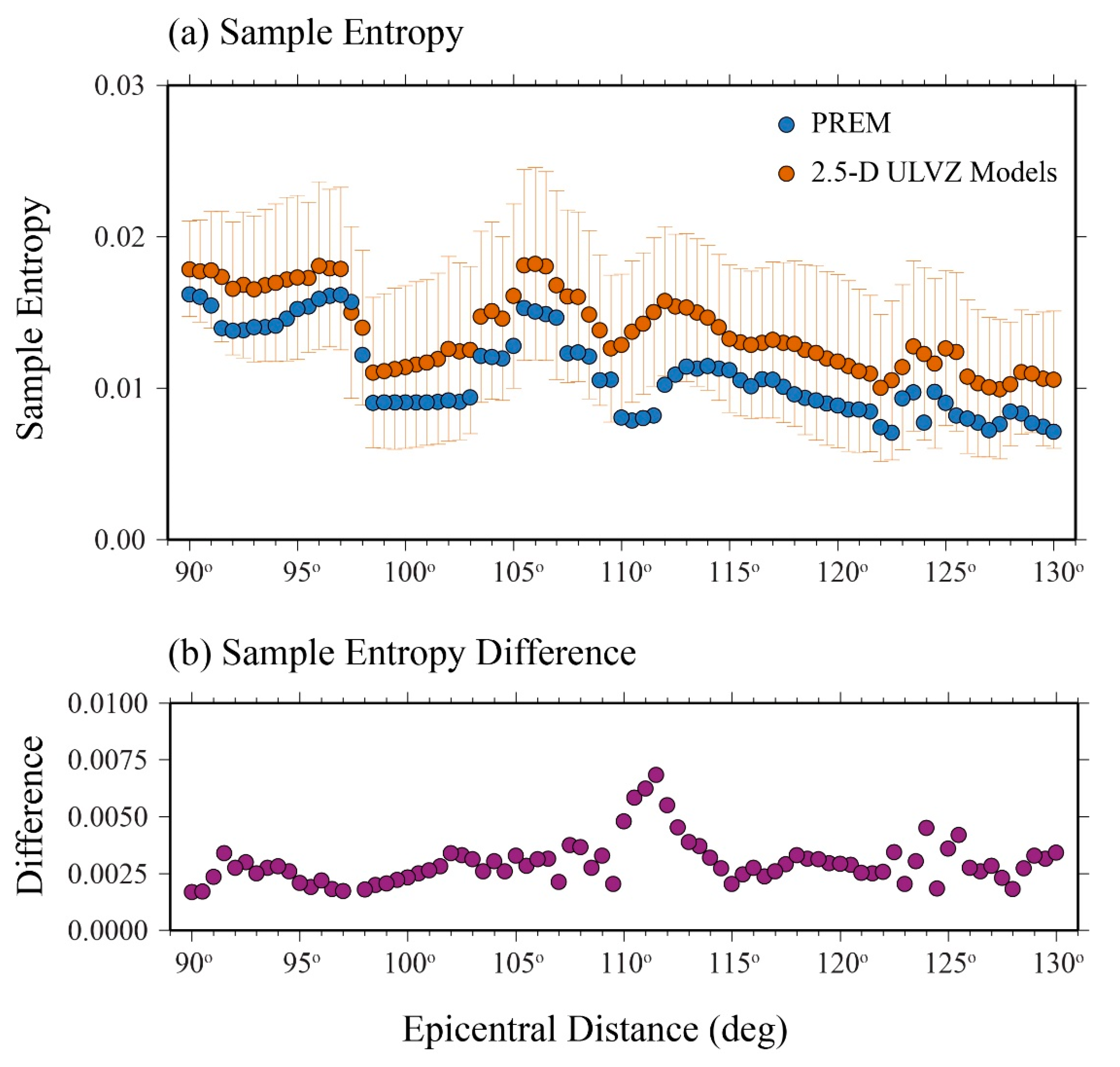
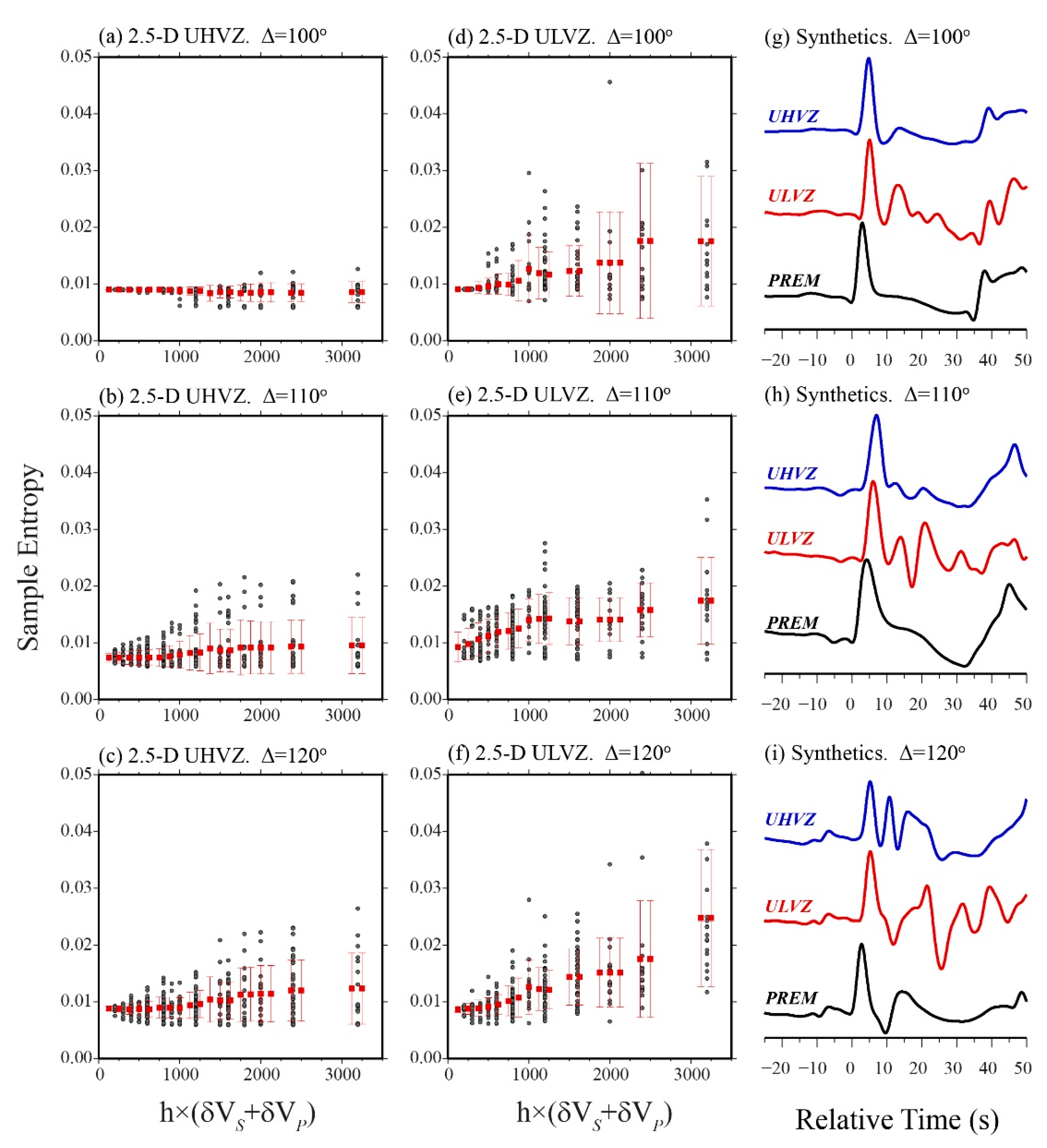
3.2. Sample Entropy of 2.5-D Models

In the previous section we showed how measurements of sample entropy varies for 1-D ULVZ and UHVZ models. However, ULVZs are not observed globally [44,89,90] but have finite dimensions [26,87,91]. In order to assess the effect of finite ULVZ/UHVZ size on SE measurements, we computed synthetic seismograms using the 2.5-D axi-symmetric finite difference (PSVaxi) code [51,92,93]. The models are here considered as 2.5-D as opposed to 2-D as in the axi-symmetric method the models are virtually rotated around a line passing through the source and the center of the Earth, which preserves correct 3-D geometrical spreading [94]. We computed synthetics for ULVZ and UHVZ models characterized by box-car shapes with different lengths (l) and left-edge positions (Δedge) in the great circle arc distance. The nomenclature we use for ULVZ or UHVZ heterogeneities is shown in Figure 5. In this example, we have drawn a heterogeneity located at Δedge = 16°, with a length of l = 6°, and a height of h = 25 km. All synthetics are computed for a 500 km source depth. Box-car shaped ULVZ models may not be the most realistic shape from a geodynamic consideration [53,95,96]. However, previous studies have investigated the effect of ULVZ shape on the SPdKS waveform and have concluded that different shapes such as trapezoidal or Gaussian shaped models do not have a strong effect on the waveform shape [97]. This is likely due to the large horizontal to vertical scale of ULVZs considered. For example, in this study the horizontal scale of the ULVZ models considered is between 180 and 730 km, and the vertical scale has a maximum thickness of 45 km.

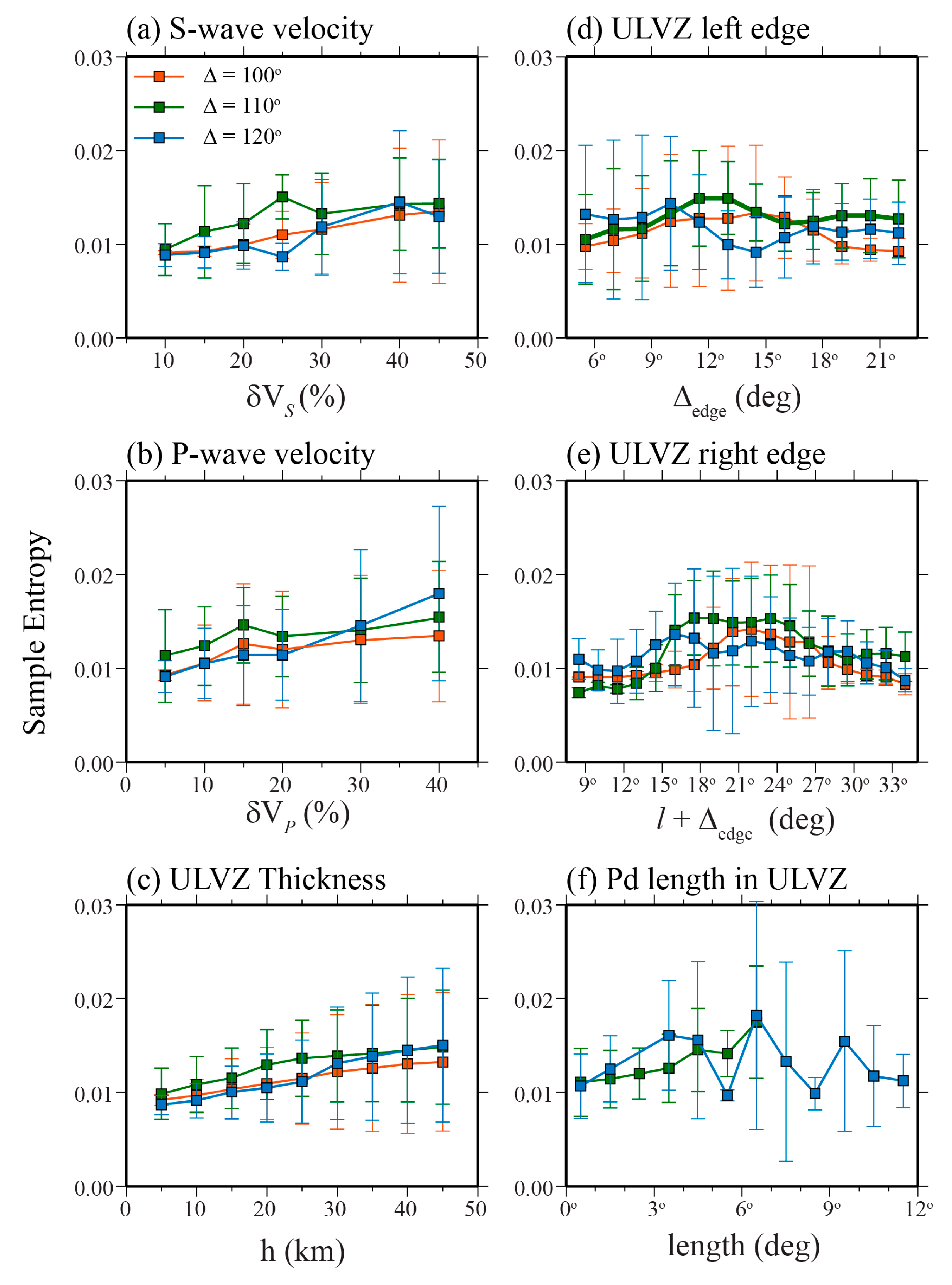
3.2.1. Sample Entropy of ULVZ Models in 2.5-D

We evaluate SE in a large suite of 2.5-D ULVZ box-car shaped models that have been computed in part for a series of previous studies [26,51,91] but significantly expanded upon here. The model space is computed for ULVZs with the following characteristics: (1) We allowed δVS decreases of 10%, 20%, 30%, and 40%. (2) We allowed δVP decreases of 0, 10%, 20%, 30%, and 40% but the magnitude of the decrease is not allowed to exceed the δVS decrease. These combinations of velocity decreases allow for 1:1, 2:1, 3:1 and 4:1 S-wave to P-wave velocity ratios. (3) We also allow for additional 3:1 S-wave to P-wave velocity ratio decreases of δVS = −15% and δVP = −5%, and δVS = −45% and δVP = −15%, which are not included in the 10% increments described above. (3) We used lengths in great circle arc direction of l = 3°, 6°, and 12°. (4) We allowed thicknesses of h = 5 to 45 km in 5 km increments. (5) We allow edge positions from Δedge = 5° to 22° in 1.5° increments. All models were computed with a fixed density increase of +10%. Our 2.5-D ULVZ model space includes 5826 ULVZ models.
We show SE for the 2.5-D models as a function of ULVZ strength in Figure 6. The axis range in Figure 6 is identical to that for Figure 3d–f so that direct comparison between 1-D and 2.5-D models is facilitated. The 1-D ULVZ models tend to display a greater average increase in SE as a function of ULVZ strength. However, some of the individual 2.5-D models display greater SE than any of the 1-D models. Nonetheless, we see that in the 2.5-D models, similarly to the 1-D models, there is a general trend towards increased SE as a function of ULVZ strength, which is most pronounced for the largest epicentral distances. We note that the uncertainties for the 2.5-D models is much larger than for the 1-D models because in 2.5-D the heterogeneity is finite in the great circle arc direction, and the SKS/SPdKS wavefield may in some cases have limited interaction with the heterogeneity.
The large number of 2.5-D ULVZ models for which we have synthetics allows us to probe the model space in greater detail, as shown in Figure 7. In this figure, for simplicity, we only show the averages and standard deviations of SE. Figure 7 shows that there is a general increase in SE as a function of S-wave velocity (Figure 7a), P-wave velocity (Figure 7b), and ULVZ thickness (Figure 7c) for the three epicentral distances. There is also a linear increase in SE as a function of ULVZ length (l), which is not shown in Figure 7. Figure 7d–f show the effect of the interaction of SKS and SPdKS with the edge of the finite length ULVZ for the same three epicentral distances.
The relationship between the SE and ULVZ position is complicated as shown in Figure 7d,e. Here, we average the SE as a function of either the left-edge of the ULVZ (i.e., Δedge) or by the right-edge of the ULVZ (i.e., l + Δedge). If only the SKS and SPdKS arrivals were present, the interpretation may be more straightforward. However, as shown in the figures and supplemental animation in Thorne et al. [58], when the down-going S-wave field interacts with the ULVZ, several additional arrivals are generated within the ULVZ and at the ULVZ boundaries. The complicated nature of all the additional arrivals makes direct interpretation of Figure 7d,e challenging.
In these experiments for 2.5-D ULVZs, we observe a maxima in SE when Δedge is near 15° (Figure 7d—red line) at an epicentral distance of 100° (no SPdKS arrival, solely SKS in PREM). From Figure 5, we can see that for an SKS arrival at 100° the left edge of the ULVZ and the down-going SKS ray path should intersect. Thus, the observed maximum in SE could be due to SKS multi-pathing. However, that interpretation is likely too simplistic, because we do not see a comparable maximum when the ULVZ right edge is near 14° (Figure 7e). However, some of the ULVZ models do generate new arrivals associated with the ULVZ edges that can show up as an SKS post-cursor at these distances. So, it is likely that the SE increase is also complicated by these additional arrivals.
For records at an epicentral distance of 110°, we also see an increase in SE beginning at Δedge = 9° that has a maxima near Δedge = 14° (Figure 7d—green line) but is back to its average level by Δedge = 17°. With respect to the ULVZ right edge, we see a broad maxima in SE from roughly Δedge + l from 17° to 25° (Figure 7e—green line). For the 500 km deep source, the initiation of Pd on the CMB occurs at an angular distance of roughly 12.8°, which subsequently exits the CMB at a distance of 19.1°. So, we tend to see an increase in the SE when the Pd path encounters the ULVZ, but the increase in complexity is likely also complicated by the constructive and destructive interference of additional arrivals created in the ULVZ.
The SE is similarly complicated at an epicentral distance of 120° but the maxima in SE tend to be shifted toward longer angular distances. For example, the SE does not start to rise until the ULVZ right edge is at Δedge + l = 18°. This may be due to the timing of the arrivals that are generated near the ULVZ right edge. If those arrivals are generated closer to the location where Pd exits the mantle, they may arrive closer to the SPdKS arrival and influence the SE measurement.
In Figure 7f, we plot SE as a function of the Pdiff portion of SPdKS within the ULVZ. For this source depth (500 km), Pd diffraction on the CMB initiates at an angular distance of 12.8° from the source. At an epicentral distance of 110°, Pd exits the CMB at 19.1°, so the maximum Pd length along the CMB is 6.3°. At an epicentral distance of 120°, Pd exits the CMB at 29.1°, and thus, the maximum Pd length along the CMB is 16.3°. However, the largest ULVZ we consider here is 12° in length, which is why this is the largest Pd path length we show in Figure 7f. For records with an epicentral distance of 110°, we see a general increase in SE as the Pd length in the ULVZ increases from 0° to 6.3°. At an epicentral distance of 120°, there appears to be a maxima in SE for a Pd path length of roughly 7°. These examples show that the SE is not just a function of the Pd path length within the ULVZ, and it is likely that the creation of additional arrivals at the ULVZ boundaries contributes the most waveform complexity in 2.5-D models (Figure 3) [58]. Thus, for 2.5-D ULVZ models, the SE is more complicated than predicted by the ULVZ strength as boundary interactions with the heterogeneity add significantly to the SE.
Thorne and Garnero [44] compared cross-correlations of SPdKS records with synthetics for the PREM model and for best-fitting 1-D ULVZ models. They found that between epicentral distance of 110° to 115° there was the largest spread in cross-correlation coefficients and used this to argue that this limited distance range may be the most diagnostic of ULVZ presence. Subsequently, highly anomalous SPdKS records in the distance range of 106° to 115° were used to map ULVZs because of the clear identification of large amplitude ULVZ-related arrivals in this distance range [52,58,59]. Here, we also examine the SE of all 2.5-D ULVZ models as a function of epicentral distance, which is shown in Figure 8. The SE as a function of distance for PREM (blue circles) and the average of all 2.5-D ULVZ models (orange circles) is shown in Figure 8a. Here, we see distinct variations as a function of distance. For example, for epicentral distances less than 98° there is generally a high SE. This is because in the time window used (−25 to +50 s with respect to SKS) an extra arrival, the direct S-wave arrival, is within the measurement window. For distances greater than 100°, the SKKS arrival starts to increase in amplitude, but exits the time window around 108°. This generates an increase in SE for all models with a maxima near 107°. This extra arrival makes the average SE larger than that measured at larger distances. Typically, the SPdKS arrival starts to emerge from the shoulder of SKS at a distance around 112°. In the PREM model, we see that the SE starts to increase here. When a ULVZ is present, SPdKS tends to emerge at an earlier distance, which manifests in a shift in the peak SE to slightly shorter distances. This is most pronounced when considering the difference in SE as a function of distance, as shown in Figure 8b. Here, commensurate with the previous studies, we see the largest change in SE with respect to PREM in the 110° to 115° distance range, and thus, this distance range may be most diagnostic for ULVZ presence using SE method as well. However, the SE average of the 2.5-D ULVZ models is almost always greater than that of PREM at all distances. Thus, the SE method shows promise in that ULVZ detection is possible at every distance.

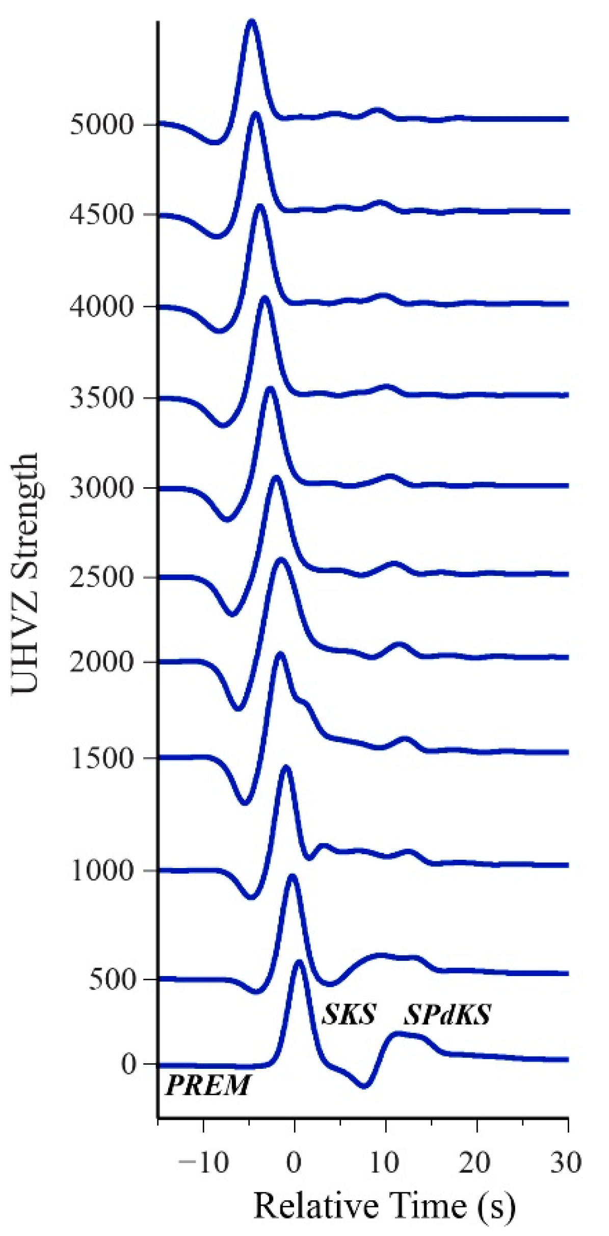
3.2.2. Sample Entropy of UHVZ Models in 2.5-D

Unlike our 2.5-D model space for ULVZs, we do not have an extensive library to draw on for UHVZs. Hence, we computed synthetics for a suite of 430 models with the following parameters: (1) We allowed δVS increases of 10, 20, 30, and 40%; (2) we allowed δVP increases of 10, 20, 30, and 40% but did not allow δVP to exceed δVS; (3) we used lengths in great circle arc direction of l = 3° and 6°; (4) we allowed a thickness of h = 10, 20, 30, and 40 km, (5) with edge positions from Δedge = 5° to 20° in 3° increments. All models were computed with a fixed density increase of +10%. The SE measurements for the 2.5-D UHVZs are shown in Figure 9a–c (using the same values of r = 0.2, and m = 2). For direct comparison with ULVZs, the same 430 models with velocity reductions as opposed to velocity increases are shown in Figure 9d,e. Example synthetic seismograms at three epicentral distances are shown in Figure 9f,g for the PREM model (black traces), a ULVZ model (red traces; δVS = δVP = −40%, h = 40 km, l = 6°, and Δedge = 17°), and a UHVZ model (blue traces δVS = δVP = +40% and other parameters the same as the ULVZ model). This model was selected because this UHVZ model displayed the largest SE at a distance of 120°.
These measurements suggest that the average SE for ULVZs is higher than for UHVZs. At an epicentral distance of 100°, the UHVZs show little increase in SE over PREM, whereas many ULVZ models show a striking increase. Measurements at these shortest distances may be diagnostic of ULVZ versus UHVZ structures. However, at larger distances (e.g., ≥110°), some UHVZ models also show substantial increases in SE comparable to that of the ULVZ models. Hence, at the larger distances, we may not be able to distinguish between ULVZ or UHVZ structure based on SE measurements of the seismic waveforms we analyzed. This contrasts with the 1-D models in which UHVZs displayed more simple waveform behavior. This is because in 2.5-D models the box-car shaped UHVZs produce additional arrivals from the edges of the UHVZs, which are not generated in the 1-D models, thus increasing the complexity of the wavefield.

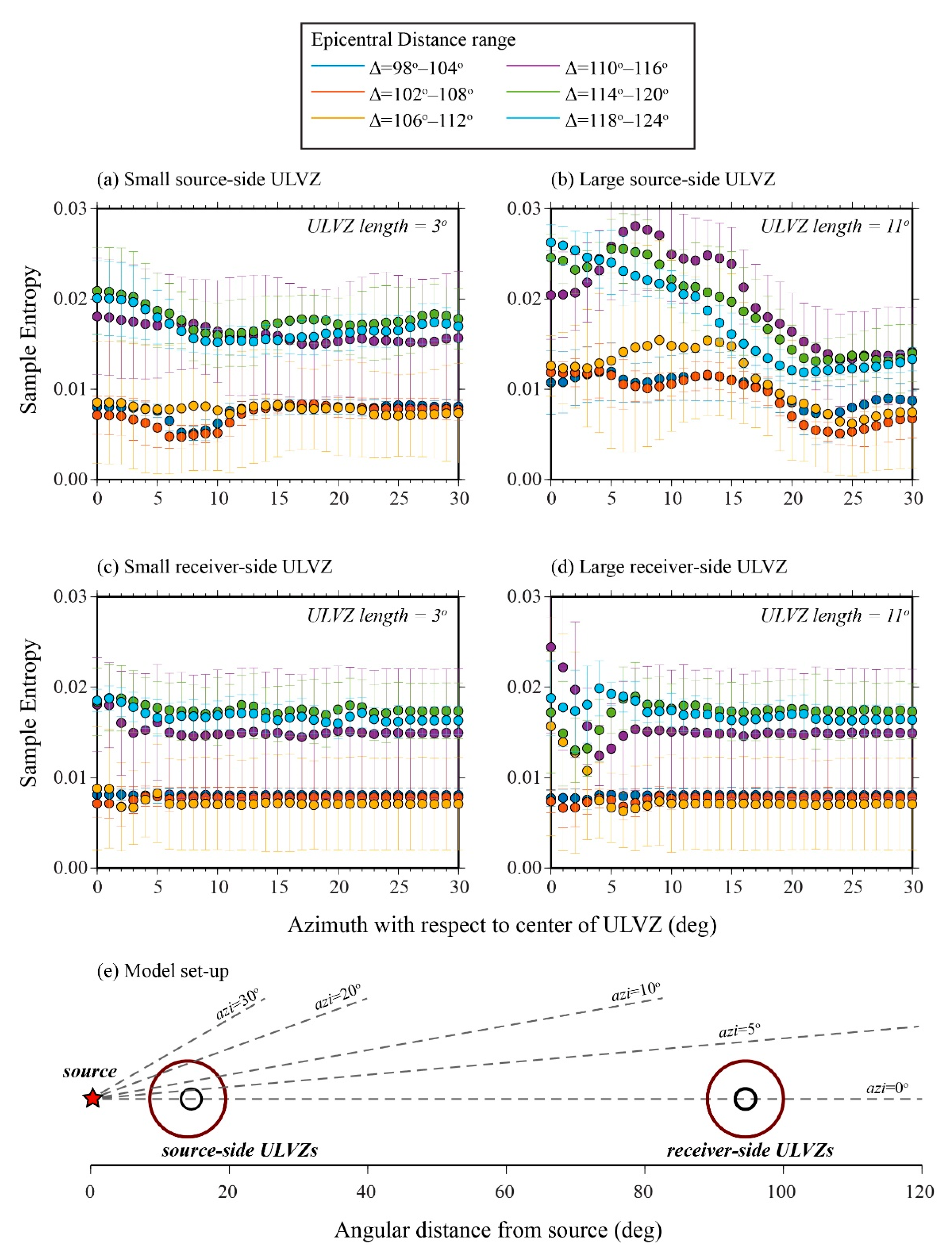
3.3. Sample Entropy of 3-D ULVZ Models

It is now possible to compute synthetic seismograms at high frequencies for fully 3-D ULVZ models. Thorne et al. [59] showed synthetic seismograms for four disk-shaped ULVZ models. These synthetics were computed for small (l = 3°) or large (l = 11°) ULVZs located on either the source- or receiver-side of the path (Figure 10e). We computed the SE for these four models and display the results as a function of azimuth in Figure 10. Here, an azimuth of 0° is for the great circle path which passes through the center of the ULVZ. Seismograms were computed for azimuths from 0° to 30° with respect to a great circle arc path passing through the center of the ULVZ. A Pdiff ray at an azimuth of 30° passes just outside of the larger (l = 11°) ULVZ. Results are grouped into six epicentral distance bands. The relationship between azimuth and SE is complex, but we can summarize the results as follows. (1) For a small source-side ULVZ, we can see effects on the SE for a wide range of azimuths. For example, for distances larger than roughly 110°, we see an increase in sample entropy at an azimuth of 0°, which decreases to approximately the baseline entropy level around an azimuth of 11°. (2) For a large source-side, ULVZ perturbations to the SE can be observed at almost all azimuths considered. Here, the SE does not appear to start leveling off until an azimuth of about 25°. (3) For a small receiver-side ULVZ, there is little effect on the SE, although a slight increase from the baseline levels may be seen at azimuths from approximately 0°–5° for the larger epicentral distances. (4) For a large receiver-side ULVZ, we see a significant effect on the SE, albeit on narrower range of azimuths than for the source-side ULVZ. From these observations, we may suggest, similarly to SPdKS waveform effects, SE increases are more likely to be observed for ULVZs that exist on the source-side of the path. However, a large ULVZ on the receiver-side of the path may also introduce an SE increase that can be measured on more than a single seismic receiver.

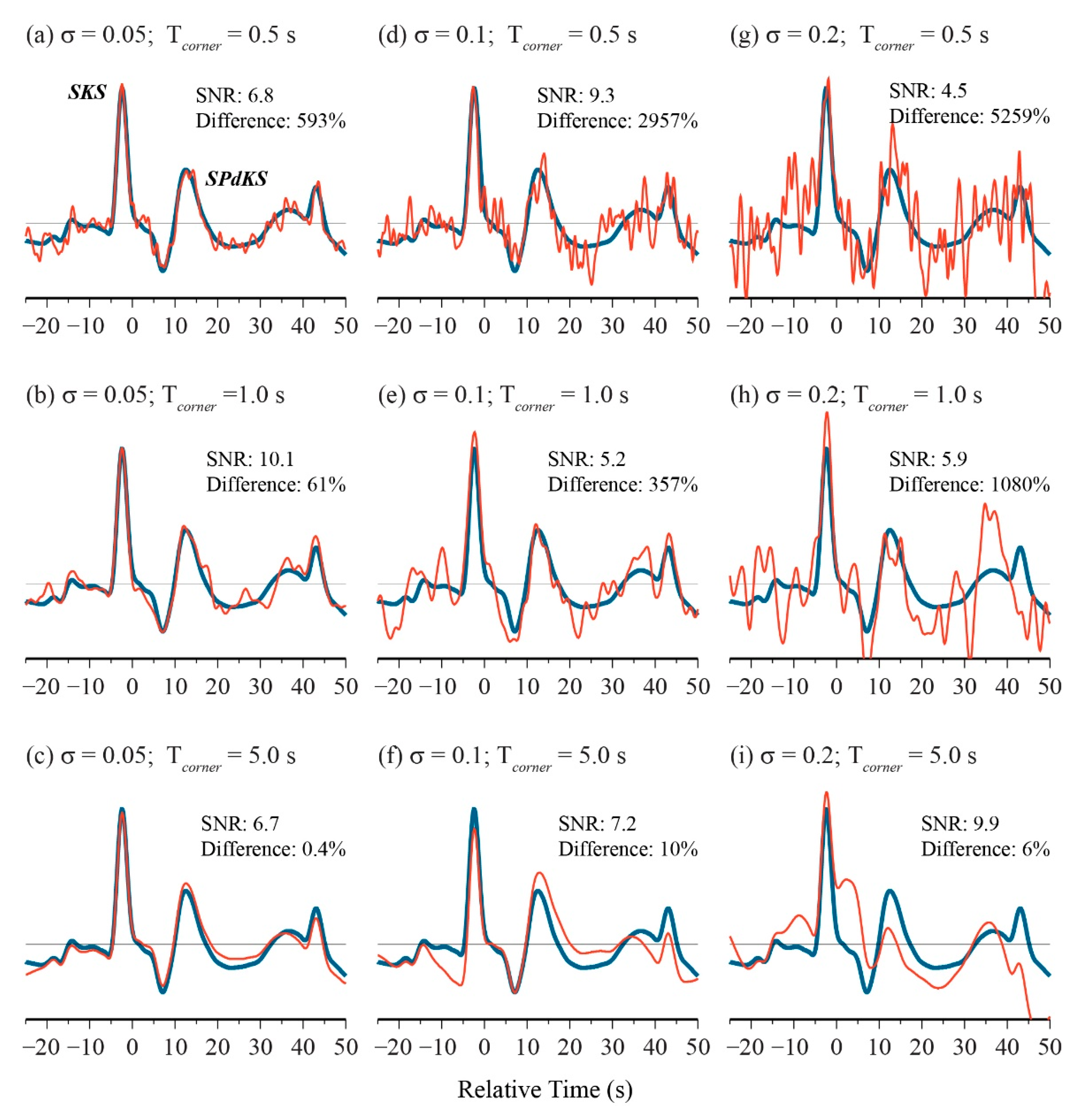
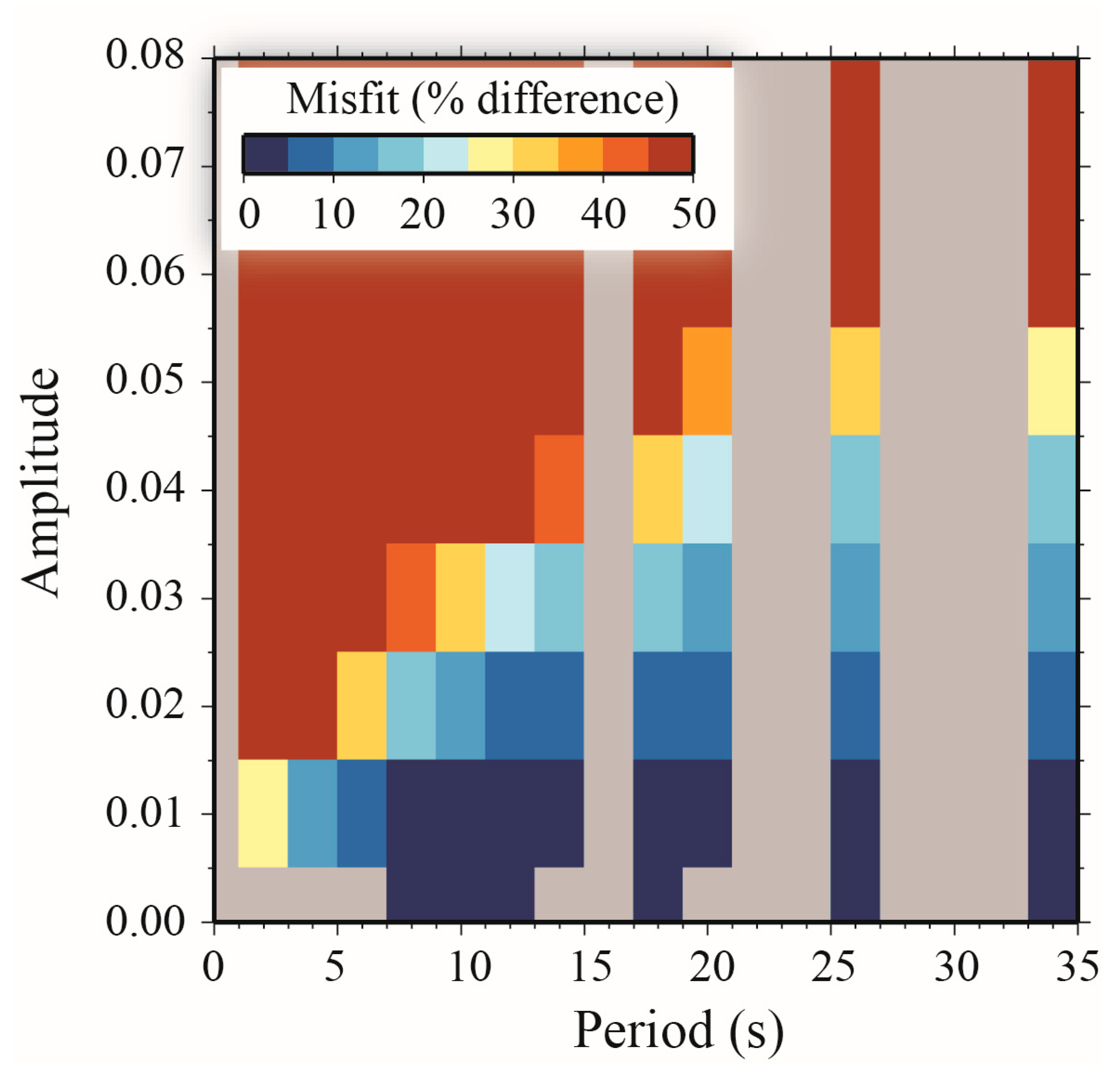
3.4. Effect of Noise

The examples shown above indicate that the idea of SE may be of interest in ULVZ studies. However, those examples were based solely on synthetic seismograms without added noise. Real seismic waveforms have noise which affects the SE measurements. Examination of the SKS and SPdKS wavefield is typically performed in the passband from roughly 1 to 50 s, but this is an exceptionally noisy part of the seismic wavefield as the ocean generated microseism band occurs in the period range from roughly 2 to 20 s [98,99]. To test the effect of noise on our SE measurements, we prepared a series of synthetic seismograms with added noise and compared the SE measurements we made on both the noisy and original seismograms.
We constructed random noise to add to our synthetic seismograms by convolving a Gaussian auto-correlation function (ACF) with a series of random numbers [100]. Here, we defined the Gaussian auto-correlation function as:
ACF t = σ e t 2 / T c o r n e r 2 ,
where T c o r n e r is the corner period and σ is the standard deviation, or root-mean square (RMS) of the noise. For periods less than T c o r n e r , the amplitude of the noise decays as governed by the Gaussian function. Some examples of noisy seismograms generated in this manner are shown in Figure 11. In this example, we repeat in all panels a single synthetic seismogram, drawn in blue, without added noise computed for a 2.5-D ULVZ model at an epicentral distance of 120°. Each column of this figure shows increasing noise amplitude ( σ   = 0.05, 0.1, and 0.2), and each row shows increasing period of the correlation length ( T c o r n e r = 0.5, 1, and 5 s). We measured the SE of each trace and report the percent difference between noisy and clean signal. In addition, we estimated the signal-to-noise ratio (SNR) of each noisy synthetic because the SNR is a commonly used metric of signal quality. As can be seen in this Figure, simple use of a SNR is not an adequate measure of how well the SE method might perform. For example, we show a case in Figure 11a where we have low noise amplitude at high frequency. This case gives us a SNR of 6.8 and a percent difference in SE of 593%. However, we obtain a percent difference in SE of only 0.4% for a similar SNR of 6.7 that has longer period noise (Figure 11c). This demonstrates that SE measurements made on seismograms with longer period and lower amplitude noise are more similar to that without noise. Thus, in order to determine which seismic data to use in measuring SE, we should consider both amplitude and period of noise present.
We can quantify which data are useable by adding noise to the synthetic seismograms prepared for our 2.5-D model space. An example is shown in Figure 12. In this example, we considered seismograms at 120° epicentral distance for each 2.5-D model with length (l) = 3° and computed five realizations of random noise for a series of RMS and Tcorner values. Tcorner values used were 0.5, 1.0, 2.0, 4.0, 6.0, and 8.0 s. RMS values used were 0.0125, 0.025, 0.05, 0.1, 0.2, and 0.4. As in the previous example, we measured the SE of the noisy trace with respect to the clean trace. In order to have a direct measurement of the noise level that can be extracted from real data, we measured the amplitude spectrum in a 100 s time window (−120 s to −20 s) ahead of the SKS arrival. This time period is devoid of other seismic arrivals on the radial component. We picked the peak amplitude and period at which the peak occurs in the amplitude spectrum, and the average percent difference in all ULVZ models are plotted in Figure 12. This figure offers a guide as to which noise levels in data may be acceptable for use in the SE method. For example, if the noise amplitude is less than 0.015, then on average, we can expect the percent misfit to be less than 5%. Therefore, if we regard 5% misfit as acceptable, we can consider many real observations for SE measurement. In practice, this level of noise should be attainable in real data as we mostly encounter longer period noise when analyzing SKS and SPdKS data because we filter out the shorter periods. For example, in [58,59], all SKS and SPdKS data were bandpass filtered with corner periods between 6 and 40 s.

4. Synthetic Analysis of Multi-Scale and Composite Multi-Scale Sample Entropy

In the previous section, we discussed measurements of SE at a single scale (scale = 1). However, as discussed in Section 2.2, we can calculate the SE at multiple scales by first decimating the signal, either through coarse-graining or through a moving average filter. The most common techniques used to look at multiple scales are referred to as the multi-scale sample entropy (MSE) and composite multi-scale sample entropy methods (CMSE). There are two reasons why these approaches may be useful. First, the effect of noise on the seismogram could possibly be mitigated, and second, patterns in the multi-scale measurements may be diagnostic of certain ULVZ features. In this section, we explore their application to our synthetic database.
Several papers explore the effects of noise on multi-scale methods [83,101]. What is observed is that for Gaussian (white) noise the SE decreases as a function of scale. For 1/f (pink) noise, where f is frequency, the SE typically remains constant as a function of scale, whereas for 1/f2 (brown) noise, the SE increases as a function of scale. It may be possible to see all of these types of noise in the seismic band used to study SKS and SPdKS. Since seismic noise in this band is so complicated, we instead focus on the lowest noise amplitudes and longer period seismic signals where the effect of noise is the most minimal.
The MSE technique has gained much popularity because of its potential for diagnostic evaluation of health. One of the first applications was in showing that electrocardiograph (ECG) measurements of people with normal healthy hearts show a distinct pattern of SE as a function of scale relative to people with abnormal heart beats such as caused by atrial fibrillation [74]. Thus, the MSE method could potentially be applied to ECG data as a diagnostic tool for assessing heart health. Since the pioneering studies by Costa et al. [74], the MSE entropy method has found numerous applications [102].

4.1. MSE and CMSE of 1-D ULVZ Models

Our first experiment is to examine our collection of 1-D synthetics as a function of ULVZ strength using the same models as in Section 3.1. We grouped our synthetics in terms of ULVZ strength and computed the MSE and CMSE using both the coarse-graining (Equation (3)) and moving average (Equation (5)) approaches to scaling. The results are shown in Figure 13 which show the primary characteristics of the different approaches. We do not consider 1-D UHVZ models, as discussed previously, these models show less complexity than PREM and are likely unrealistic for the Earth.
In Figure 13a, we show the MSE result using coarse-graining. For 1-D ULVZ models and the chosen parameters (r = 0.2 and m = 2), there is a general increase in SE up to scales 9 or 10 before the SE starts to decrease again. Increasing ULVZ strength increases the SE over all scales. A maximum in the difference in SE between the strength = 0 models and all other ULVZ models occurs at scale 9 or 10 where the peak in SE occurs. The CMSE (Figure 13b) shows a smoother pattern which increases as a function of scale. Considering these 1-D models, both MSE and CMSE methods could potentially be used as diagnostic of ULVZ strength. The variation across models, as represented by the standard deviation bars, is wide, but the least amount of overlap between the low and high strength ULVZ models is observed for the CMSE method at the larger scales (e.g., scale 11). Thus, the CMSE method at larger scales may be the most diagnostic of ULVZ strength.
In Figure 13c,d, we show the MSE and CMSE measurements for the case where we use the moving average filter. Here, we show the result up to scale 50. The patterns observed here are similar in shape to that of the coarse-grained result. However, in the case of the MSE (Figure 13c) the peak of the MSE curve tends to shift towards lower scales for higher ULVZ strengths. As in the coarse-grained result, the separation between low strength and high strength ULVZ models becomes larger than at scale 1, and thus, it may be useful to consider these additional scales in assessing ULVZ existence. At larger scales (e.g., scale 20 for MSE and scale 35 for CMSE), the separation between the largest strength ULVZs and the weakest ULVZs is large enough that the one standard deviation error bars do not overlap. This provides further evidence that examining these larger scales may be valuable for discrimination of heterogeneities from background mantle.

4.2. MSE and CMSE of 2.5-D ULVZ Models

We examined the MSE of our 2.5-D ULVZ model space using coarse-graining and grouping together similar ULVZ patterns. Some characteristic results are shown in Figure 14. In Figure 14a–c, we show the MSE for three epicentral distances where we have grouped models together by ULVZ thickness. We see a similar behavior at all epicentral distances where the SE increases as a function of ULVZ thickness at each scale. A peak in the MSE curve occurs at scale 8 as well as the maximum separation in SE between the thinnest and thickest ULVZ models. A similar pattern occurs, although not shown here, if we consider grouping ULVZ models by δVS, δVP, or length (l). Namely, the MSE patterns look very similar to those shown for thickness, and the SE increases at each scale with increased magnitude of δVS or δVP perturbation, or increased ULVZ length. However, we do not see any change in the pattern of the MSE curves that could be used to distinguish variation in one of these parameters.
In Figure 14d–f, we show the MSE for ULVZ models grouped by left edge (Δedge). Here, the pattern is not as simple as in the previous scenarios. At an epicentral distance of 100°, we see the largest SE across all scales for the smallest Δedge positions, whereas at 110° and 120°, there is a similar level of complexity for all Δedge positions. However, as with the previous examples, there does not appear to be a robust change in the patterns of the MSE curves that could be used to elucidate the ULVZ position. Although not shown here, MSE curves for the right edge of ULVZ (l + Δedge) shows a similar pattern.
In order to assess if the MSE technique can be diagnostic of ULVZ or UHVZ presence, we compared PREM with all 2.5-D ULVZ and UHVZ models with lengths (l) ≥ 11.0°. The larger ULVZ and UHVZ lengths were selected to be certain that the SPdKS wavefield interacted with ULVZ or UHVZ structure. The measurements are shown in Figure 15 using coarse-graining, but the results using the moving average are similar. At all distances and scales shown in Figure 15, the SE for ULVZ models is larger than that for UHVZ and PREM models. For all models, a peak in the MSE curve occurs at a scale of 8. At this scale, the largest separation between ULVZ and PREM models occurs, and thus, it may be at this scale where ULVZ presence is most well-defined for the sampling interval and threshold (r) we used in the SE measurements. At epicentral distances of 100° and 110°, the MSE curve for UHVZs and PREM models do not significantly differ. However, at an epicentral distance of 120°, the UHVZ curve is more similar to that for the ULVZ models. At all epicentral distances, the ULVZ models keep a fairly constant separation in SE from PREM for scales ≥ 8. ULVZ models also appear well separated from UHVZ models at distances of 100° and 110°. However, it may be difficult to distinguish ULVZ from UHVZ at the largest epicentral distances.
Overall, we do not find distinct MSE curve patterns that could be used to distinguish between different classes of models (e.g., UHVZ or ULVZ) such as has been done in other areas of study. However, we propose that use of the MSE technique is still beneficial as the separation between SE becomes increased at specific scales (in these examples we always see a maximum separation at scale 8). In addition, we always observe an increase in SE over that of PREM for all ULVZ models. Hence, one criterion for diagnosing ULVZ existence could be that we see an increase in SE across all scales, which may be more of a robust indicator than looking at just a single scale.

5. Conclusions

We have presented a synthetic analysis of utilizing SE-based techniques to analyze seismic waveforms in the vicinity of the SKS and SPdKS time window. When anomalous lower mantle structures exist, such as ULVZ or UHVZ heterogeneity, additional seismic arrivals are generated that may increase the complexity and thus the SE of the seismic traces. Thus, we find that SE-based techniques may be useful in characterizing regions of the lowermost mantle with heterogeneous structures. It is important to note that the SE techniques examine the waveform complexity as data recorded on the surface as opposed to the wavefield complexity propagating within the Earth’s volume. Mantle heterogeneities create wavefield complexity that is reduced by the time the wavefield reaches the surface [103,104]. This wavefield complexity cannot be retrieved by surface-bound waveform measurements, but is inherent in using surface observations to constrain mantle properties.
Overall, we find that SE increases as a function of ULVZ or UHVZ strength, except for 1-D UHVZ models. That is, the SE increases as a function of the thickness and decrease in P- and/or S-wave velocity. However, the observation is dependent on where the heterogeneity is located with respect to the wavefield and at which epicentral distance the observation is made. For records at the shortest epicentral distances (e.g., near Δ = 100°), we see almost no difference in SE between UHVZ models and PREM. Hence, observations of SE increases at these shortest distances are most likely going to be associated with ULVZs. At the mid-distances (e.g., near Δ = 110°), the SE for UHVZs begins to deviate from the PREM model. However, observations at multiple scales show that the SE for ULVZ models separates substantially more from PREM. Again, at the mid-distances, increases in SE appear that they will most likely be related to ULVZ features. This is important as previous studies which have focused on records in the distances around 110° were clear to note that highly anomalous SPdKS waveforms could also be due to UHVZ phenomena. However, increased measurement of SE in these regions would likely indicate a ULVZ source. On the other hand, detections of highly anomalous SPdKS waveforms alongside little to no SE increase may be indicative of UHVZ presence. As discussed previously, the largest range in SEs occurs for records recorded in the mid-distance ranges. Interestingly, for waveforms recorded at the longest epicentral distances (e.g., near Δ = 120°), we see that features that have positions (i.e., larger Δedge positions) introduce the largest increases in SE. This may be especially useful as most previous SPdKS studies focused on shorter epicentral distance recordings. Hence, the MSE approach may provide a tool to identify ULVZ features using an expanded dataset of long-distance recordings which are sensitive to structures at the far edge of the Pd path. Nevertheless, some caution must be employed here as on average we see similar increases in SE for UHVZ models as well. However, at these large epicentral distances SPdKS is well separated from SKS and it may be possible to identify UHVZ versus ULVZ features based on differential travel-time measurements of SPdKS-SKS. These types of travel-time measurements have not been used extensively as they are challenging due to the emergent nature of the SPdKS arrival and only subtle changes in observed travel-times. However, corroborating evidence of increased SE may lend support to the existence of heterogeneities in these regions, and thus, the evidence will be more supported than from just the travel-time measurements on their own.
The SPdKS seismic phase is complicated by the concurrent existence of the SKPdS phase. In this study, we only investigated the effects of heterogeneities on the source-side of the path that would be sampled by SPdKS. However, some variation in waveforms is observed when heterogeneity exists on the receiver-side of the path. As demonstrated in Vanacore et al. [97], the main difference appears to be the existence of additional post-cursor arrivals. These additional post-cursors are yet to be observed in data, but their presence could introduce SE increases. Observations of receiver-side SE increases should be scrutinized for the presence of these post-cursors as this would provide compelling evidence of receiver-side heterogeneity.
In Section 3 of this paper, we demonstrated that single scale SE measurements can detect heterogeneous structures. However, there is little added cost to computing the SE at multiple scales, and thus, we advocate for the use of MSE and CMSE techniques. We did not observe characteristic changes in MSE curves that could be diagnostic of ULVZ versus PREM or UHVZ waveforms. Rather, what is observed at different scales is a general increase in SE between heterogeneous models and PREM up to a given scale (e.g., around scale 8 or 9 for coarse-graining or scale 20 to 25 for a moving average approach). Thus, this information at multiple scales can be used to provide greater reliability on the interpretation.
A potential drawback to the MSE method is that different types of noise affect SE measurements differently. This must be considered in any study using the MSE approach. In this paper, we considered noise with a Gaussian autocorrelation function. However, real seismic noise may behave differently. Future efforts may wish to evaluate the effects of real seismic noise added to the signals. However, for the small time-windows we are looking at in this study and within the longer period filter bands we use, we see that the effect of noise should be minimized, so long as we are careful to measure the noise characteristics of the data and exclude records in which the noise is too high. However, there is a balance between filtering out the high frequency noise that contaminates the SE measurements and the ability to resolve fine-scale heterogeneous structure. When investigating real seismic data, it may be advisable to look at seismograms in multiple frequency bands.
In this paper we focused on the effects of small-scale ULVZ and UHVZ heterogeneities. However, as discussed in the introduction other types of heterogeneities exist in the lower mantle. The large-scale structures, such as LLVPs and the D″ discontinuity, will primarily influence the SKS/SPdKS wavefield through travel-time anomalies and will not contribute to increases in SE [105]. However, sharp boundaries to these features have been reported in several studies [106,107,108,109,110,111]. These sharp boundaries could generate multi-pathed arrivals [13,107,112] which would increase the SE of signals near these boundaries. Smaller-scale structures may also be present that give rise to scattered arrivals [113]. If these structures are on the order of the wavelength of the SKS arrivals it is possible they could also contribute to increases in SE. One of the attractive features of the MSE technique is its ability to distinguish different scattering regimes [114], so this method may aid in classifying such different objects more comprehensively than conventional measurement techniques. For the long-period SKS waves we investigate in this study, the wavelength in the lower mantle is on the order of 70 km, which is larger than the scale length of scatterers inferred from recent studies [19,115]. However, this scale length of scatterers is possible within the lower mantle [116] and could also contribute to increased SE when real data are considered.
Most past SPdKS studies have focused on waveform characteristics which are most sensitive in a narrow distance range. However, the MSE technique may also be able to pick up on the more subtle SE changes across all distances. Using the data set collected in [26,58], as much as 85% of the CMB by surface area could potentially be scrutinized, whereas 57% of the CMB was covered in Thorne et al. [59] using the more limited epicentral distance range. Thus, this method could be utilized to explore a much larger range of the CMB than has been previously explored, one that is nearing global coverage. However, as noted previously, ULVZ detection will likely still be heavily weighted towards the source-side of the SPdKS/SKPdS path. In the companion paper, we apply this methodology to a global data set.

Author Contributions

Conceptualization, M.S.T. and T.N.-M.; methodology, S.P. and M.S.T.; software, S.P.; validation, S.P. and M.S.T., formal analysis, S.P. and M.S.T.; investigation, S.P.; writing—original draft preparation, S.P. and M.S.T.; writing—review and editing, S.P. and M.S.T.; visualization, S.P. and M.S.T.; supervision, M.S.T.; project administration, M.S.T.; funding acquisition, M.S.T. and T.N.-M. All authors have read and agreed to the published version of the manuscript.

Funding

This research was funded by NSF grant numbers EAR 1723081 and 2139966, and NERC grant number NE/R012199/1.

Acknowledgments

The authors acknowledge the University of Utah Center for High Performance Computing (CHPC) for computing resources and support. We thank two anonymous reviewers for constructive comments that improved this manuscript. Figures were drawn using the Generic Mapping Tools [117].

Conflicts of Interest

The authors declare no conflict of interest.

References

  1. Dziewonski, A.M.; Anderson, D.L. Preliminary reference Earth model. Phys. Earth Planet. Inter. 1981, 25, 297–356. [Google Scholar] [CrossRef]
  2. Boehler, R. Melting of the FeFeO and the FeFeS Systems at high pressure: Constraints on core temperatures. Earth Planet. Sci. Lett. 1992, 111, 217–227. [Google Scholar] [CrossRef]
  3. Lay, T.; Hernlund, J.; Buffett, B.A. Core-mantle boundary heat flow. Nat. Geosci. 2008, 1, 25–32. [Google Scholar] [CrossRef]
  4. Garnero, E.J. Heterogeneity of the lowermost mantle. Annu. Rev. Earth Planet. Sci. 2000, 28, 509–537. [Google Scholar] [CrossRef]
  5. Dziewonski, A.M.; Forte, A.M.; Su, W.; Woodward, R.L. Seismic tomography and geodynamics. In Relating Geophysical Structures and Processes: The Jeffreys Volume; Aki, K., Dmowska, R., Eds.; Washington DC American Geophysical Union Geophysical Monograph Series; American Geophysical Union: Washington, DC, USA, 1993; Volume 76, pp. 67–105. [Google Scholar]
  6. Simmons, N.A.; Forte, A.M.; Boschi, L.; Grand, S.P. GyPSuM: A joint tomographic model of mantle density and seismic wave speeds. J. Geophys. Res. Solid Earth 2010, 115, B12310. [Google Scholar] [CrossRef]
  7. Ritsema, J.; Deuss, A.; van Heijst, H.-J.; Woodhouse, J.H. S40RTS: A degree-40 shear-velocity model for the mantle from new Rayleigh wave dispersion, teleseismic traveltime and normal-mode splitting function measurements. Geophys. J. Int. 2011, 184, 1223–1236. [Google Scholar] [CrossRef] [Green Version]
  8. Koelemeijer, P.; Ritsema, J.; Deuss, A.; Van Heijst, H.-J. SP12RTS: A degree-12 model of shear- and compressional-wave velocity for Earth’s mantle. Geophys. J. Int. 2016, 204, 1024–1039. [Google Scholar] [CrossRef] [Green Version]
  9. French, S.W.; Romanowicz, B. Broad plumes rooted at the base of the Earth’s mantle beneath major hotspots. Nature 2015, 525, 95–99. [Google Scholar] [CrossRef]
  10. Houser, C.; Masters, G.; Shearer, P.; Laske, G. Shear and compressional velocity models of the mantle from cluster analysis of long-period waveforms. Geophys. J. Int. 2008, 174, 195–212. [Google Scholar] [CrossRef] [Green Version]
  11. Rao, B.P.; Kumar, M.R. Seismic evidence for slab graveyards atop the Core Mantle Boundary beneath the Indian Ocean Geoid Low. Phys. Earth Planet. Inter. 2014, 236, 52–59. [Google Scholar]
  12. Cobden, L.; Thomas, C.; Trampert, J. Seismic detection of post-perovskite inside the Earth. In The Earth’s Heterogeneous Mantle; Deschamps, F., Khan, A., Eds.; Springer Geophysics: Berlin/Heidelberg, Germany, 2015; pp. 391–440. [Google Scholar]
  13. Whittaker, S.; Thorne, M.S.; Schmerr, N.C.; Miyagi, L. Seismic array constraints on the D″ discontinuity beneath Central America. J. Geophys. Res. Solid Earth 2016, 121, 152–169. [Google Scholar] [CrossRef] [Green Version]
  14. Borgeaud, A.F.; Kawai, K.; Konishi, K.; Geller, R.J. Imaging paleoslabs in the D ′′ layer beneath Central America and the Caribbean using seismic waveform inversion. Sci. Adv. 2017, 3, e1602700. [Google Scholar] [CrossRef] [Green Version]
  15. Garnero, E.J.; McNamara, A.K.; Shim, S.-H. Continent-sized anomalous zones with low seismic velocity at the base of Earth’s mantle. Nat. Geosci. 2016, 9, 481–489. [Google Scholar] [CrossRef]
  16. Hosseini, K.; Sigloch, K.; Tsekhmistrenko, M.; Zaheri, A.; Nissen-Meyer, T.; Igel, H. Global mantle structure from multifrequency tomography using P, PP and P-diffracted waves. Geophys. J. Int. 2020, 220, 96–141. [Google Scholar] [CrossRef]
  17. Lay, T. Deep earth structure: Lower mantle and D″. In Seismology and the Structure of the Earth. Treatise on Geophysics, 2nd ed.; Schubert, G., Ed.; Elsevier: Amsterdam, The Netherlands, 2015; Volume 1. [Google Scholar]
  18. Rost, S.; Thorne, M.S.; Garnero, E.J. Imaging Global Seismic Phase Arrivals by Stacking Array Processed Short-Period Data. Seismol. Res. Lett. 2006, 77, 697–707. [Google Scholar] [CrossRef]
  19. Mancinelli, N.J.; Shearer, P.; Thomas, C. On the frequency dependence and spatial coherence of PKP precursor amplitudes. J. Geophys. Res. Solid Earth 2016, 121, 1873–1889. [Google Scholar] [CrossRef]
  20. Waszek, L.; Thomas, C.; Deuss, A. PKP precursors: Implications for global scatterers. Geophys. Res. Lett. 2015, 42, 3829–3838. [Google Scholar] [CrossRef] [Green Version]
  21. Yu, S.; Garnero, E.J. Ultralow velocity zone locations: A global assessment. Geochem. Geophys. Geosyst. 2018, 19, 396–414. [Google Scholar] [CrossRef]
  22. Wen, L. Intense seismic scattering near the Earth’s core-mantle boundary beneath the Comores hotspot. Geophys. Res. Lett. 2000, 27, 3627–3630. [Google Scholar] [CrossRef]
  23. Idehara, K.; Yamada, A.; Zhao, D. Seismological constraints on the ultralow velocity zones in the lowermost mantle from core-reflected waves. Phys. Earth Planet. Inter. 2007, 165, 25–46. [Google Scholar] [CrossRef]
  24. Pachhai, S.; Dettmer, J.; Tkalčić, H. Ultra-low velocity zones beneath the Philippine and Tasman Seas revealed by a trans-dimensional Bayesian waveform inversion. Geophys. J. Int. 2015, 203, 1302–1318. [Google Scholar] [CrossRef]
  25. Cottaar, S.; Romanowicz, B. An unsually large ULVZ at the base of the mantle near Hawaii. Earth Planet. Sci. Lett. 2012, 355, 213–222. [Google Scholar] [CrossRef]
  26. Krier, J.; Thorne, M.S.; Leng, K.; Nissen-Meyer, T. A compositional component to the Samoa ultralow-velocity zone revealed through 2- and 3-D waveform modeling of SKS and SKKS differential travel-times and amplitudes. J. Geophys. Res. Solid Earth 2021, 126, e2021JB021897. [Google Scholar] [CrossRef]
  27. Jenkins, J.; Mousavi, S.; Li, Z.; Cottaar, S. A high-resolution map of Hawaiian ULVZ morphology from ScS phases. Earth Planet. Sci. Lett. 2021, 563, 116885. [Google Scholar] [CrossRef]
  28. McNamara, A.K. A review of large low shear velocity provinces and ultra low velocity zones. Tectonophysics 2019, 760, 199–220. [Google Scholar] [CrossRef]
  29. Ma, X.; Sun, X.; Thomas, C. Localized ultra-low velocity zones at the eastern boundary of Pacific LLSVP. Earth Planet. Sci. Lett. 2019, 507, 40–49. [Google Scholar] [CrossRef]
  30. Garnero, E.J.; Helmberger, D.V. A very slow basal layer underlying large-scale low-velocity anomalies in the lower mantle beneath the Pacific: Evidence from core phases. Phys. Earth Planet. Inter. 1995, 91, 161–176. [Google Scholar] [CrossRef]
  31. Choy, G.L. Theoretical seismograms of core phases calculated by frequency-dependent full wave theory, and their interpretation. Geophys. J. Roy. Astron. Soc. 1977, 51, 275–311. [Google Scholar] [CrossRef] [Green Version]
  32. Kohler, M.D.; Vidale, J.E.; Davis, P.M. Complex scattering within D” observed on the very dense Los Angeles Region Seismic Experiment passive array. Geophys. Res. Lett. 1997, 24, 1855–1858. [Google Scholar] [CrossRef] [Green Version]
  33. Hutko, A.R.; Lay, T.; Revenaugh, J. Localized double-array stacking analysis of PcP: D” and ULVZ structure beneath the Cocos plate, Mexico, central Pacific, and north Pacific. Phys. Earth Planet. Inter. 2009, 173, 60–74. [Google Scholar] [CrossRef]
  34. Garnero, E.J.; Vidale, J.E. ScP; a probe of ultralow velocity zones at the base of the mantle. Geophys. Res. Lett. 1999, 26, 377–380. [Google Scholar] [CrossRef] [Green Version]
  35. Hansen, S.E.; Carson, S.E.; Garnero, E.J.; Rost, S.; Yu, S. Investigating ultra-low velocity zones in the southern hemisphere using an Antarctic dataset. Earth Planet. Sci. Lett. 2020, 536, 116142. [Google Scholar] [CrossRef]
  36. Ni, S.; Helmberger, D.V. Horizontal transition from fast to slow structures at the core-mantle boundary; South Atlantic. Earth Planet. Sci. Lett. 2001, 187, 301–310. [Google Scholar] [CrossRef]
  37. Thomas, C.; Weber, M.; Wicks, C.W.; Scherbaum, F. Small scatterers in the lower mantle observed at German broadband arrays. J. Geophys. Res. 1999, 104, 15073–15088. [Google Scholar] [CrossRef]
  38. Thomas, C.; Kendall, J.-M.; Helffrich, G. Probing two low-velocity regions with PKP b-caustic amplitudes and scattering. Geophys. J. Int. 2009, 178, 503–512. [Google Scholar] [CrossRef] [Green Version]
  39. Rondenay, S.; Fischer, K.M. Constraints on localized core-mantle boundary structure from multichannel, broadband SKS coda analysis. J. Geophys. Res. 2003, 108, 2537. [Google Scholar] [CrossRef] [Green Version]
  40. Kim, D.; Lekic, V.; Menard, B.; Baron, D.; Taghizadeh-Popp, M. Sequencing seismograms: A panoptic view of scattering in the core-mantle boundary region. Science 2020, 368, 1223–1228. [Google Scholar] [CrossRef]
  41. Yuan, K.; Romanowicz, B. Seismic evidence for partial melting at the root of major hot spot plumes. Science 2017, 357, 393–397. [Google Scholar] [CrossRef] [Green Version]
  42. Xu, Y.; Koper, K.D. Detection of a ULVZ at the base of the mantle beneath the northwest Pacific. Geophys. Res. Lett. 2009, 36, L17301. [Google Scholar] [CrossRef] [Green Version]
  43. Rost, S.; Garnero, E.J. Detection of an ultralow velocity zone at the core-mantle boundary using diffracted PKKPab waves. J. Geophys. Res. 2006, 111, B07309. [Google Scholar] [CrossRef] [Green Version]
  44. Thorne, M.S.; Garnero, E.J. Inferences on ultralow-velocity zone structure from a global analysis of SPdKS waves. J. Geophys. Res. 2004, 109, B08301. [Google Scholar] [CrossRef]
  45. Luo, S.-N.; Ni, S.; Helmberger, D.V. Evidence for a sharp lateral variation of velocity at the core–mantle boundary from multipathed PKPab. Earth Planet. Sci. Lett. 2001, 189, 155–164. [Google Scholar] [CrossRef]
  46. Vidale, J.E.; Hedlin, M.A. Evidence for partial melt at the core–mantle boundary north of Tonga from the strong scattering of seismic waves. Nature 1998, 391, 682–685. [Google Scholar] [CrossRef]
  47. Garnero, E.J.; Revenaugh, J.; Williams, Q.; Lay, T.; Kellogg, L.H. Ultralow velocity zone at the core-mantle boundary. In The Core-Mantle Boundary Region; American Geophysical Union: Washington, DC, USA, 1998; Volume 28, pp. 319–334. [Google Scholar]
  48. Pachhai, S.; Tkalčić, H.; Dettmer, J. Bayesian inference for ultralow velocity zones in the Earth’s lowermost mantle: Complex ULVZ beneath the east of the Philippines. J. Geophys. Res. Solid Earth 2014, 119, 8346–8365. [Google Scholar] [CrossRef]
  49. Wen, L.; Helmberger, D.V. Ultra-low velocity zones near the core-mantle boundary from broadband PKP precursors. Science 1998, 279, 1701–1703. [Google Scholar] [CrossRef] [Green Version]
  50. Rondenay, S.; Cormier, V.F.; Van Ark, E.M. SKS and SPdKS sensitivity to two-dimensional ultralow-velocity zones. J. Geophys. Res. Solid Earth 2010, 115, B04311. [Google Scholar] [CrossRef]
  51. Thorne, M.S.; Garnero, E.J.; Jahnke, G.; Igel, H.; McNamara, A.K. Mega ultra low velocity zone and mantle flow. Earth Planet. Sci. Lett. 2013, 364, 59–67. [Google Scholar] [CrossRef]
  52. Thorne, M.S.; Takeuchi, N.; Shiomi, K. Melting at the edge of a slab in the deepest mantle. Geophys. Res. Lett. 2019, 46, 8000–8008. [Google Scholar] [CrossRef]
  53. Pachhai, S.; Li, M.; Thorne, M.S.; Dettmer, J.; Tkalčić, H. Internal structure of ultralow-velocity zones consistent with origin from a basal magma ocean. Nat. Geosci. 2022, 15, 79–84. [Google Scholar] [CrossRef]
  54. Williams, Q.; Garnero, E.J. Seismic evidence for partial melt at the base of Earth’s mantle. Science 1996, 273, 1528–1530. [Google Scholar] [CrossRef] [Green Version]
  55. Berryman, J.G. Seismic velocity decrement ratios for regions of partial melt in the lower mantle. Geophys. Res. Lett. 2000, 27, 421–424. [Google Scholar] [CrossRef]
  56. Williams, Q.; Revenaugh, J.; Garnero, E. A correlation between ultra-low basal velocities in the mantle and hot spots. Science 1998, 281, 546–549. [Google Scholar] [CrossRef] [PubMed]
  57. Niu, F.; Wen, L. Strong seismic scatterers near the core-mantle boundary west of Mexico. Geophys. Res. Lett. 2001, 28, 3557–3560. [Google Scholar] [CrossRef] [Green Version]
  58. Thorne, M.S.; Pachhai, S.; Leng, K.; Wicks, J.K.; Nissen-Meyer, T. New candidate ultralow-velocity zone locations from highly anomalous SPdKS waveforms. Minerals 2020, 10, 211. [Google Scholar] [CrossRef] [Green Version]
  59. Thorne, M.S.; Leng, K.; Pachhai, S.; Rost, S.; Wicks, C.W.; Nissen-Meyer, T. The most parsimonious ultralow-velocity zone distribution from highly anomalous SPdKS waveforms. Geochem. Geophys. Geosyst. 2021, 22, e2020GC009467. [Google Scholar] [CrossRef]
  60. Andrault, D.; Pesce, G.; Bouhifd, M.A.; Bolfan-Casanova, N.; Hénot, J.-M.; Mezouar, M. Melting of subducted basalt at the core-mantle boundary. Science 2014, 344, 892–895. [Google Scholar] [CrossRef]
  61. Wicks, J.; Jackson, J.; Sturhahn, W. Very low sound velocities in iron-rich (Mg, Fe) O: Implications for the core-mantle boundary region. Geophys. Res. Lett. 2010, 37, L15304. [Google Scholar] [CrossRef] [Green Version]
  62. Wicks, J.K.; Jackson, J.M.; Sturhahn, W.; Zhang, D. Sound velocity and density of magnesiowüstites: Implications for ultralow-velocity zone topography. Geophys. Res. Lett. 2017, 44, 2148–2158. [Google Scholar] [CrossRef]
  63. Finkelstein, G.J.; Jackson, J.M.; Said, A.; Alatas, A.; Leu, B.M.; Sturhahn, W.; Toellner, T.S. Strongly anisotropic magnesiowüstite in Earth’s lower mantle. J. Geophys. Res. Solid Earth 2018, 123, 4740–4750. [Google Scholar] [CrossRef]
  64. Jackson, J.M.; Thomas, C. Seismic and mineral physics constraints on the D″ layer. In Mantle Convection and Surface Expressions; Marquardt, H., Ballmer, M., Cottaar, S., Konter, J., Eds.; American Geophysical Union: Washington, DC, USA, 2021. [Google Scholar] [CrossRef]
  65. Mao, W.L.; Mao, H.-k.; Sturhahn, W.; Zhao, J.; Prakapenka, V.B.; Meng, Y.; Shu, J.; Fei, Y.; Hemley, R.J. Iron-rich post-perovskite and the origin of ultralow-velocity zones. Science 2006, 312, 564–565. [Google Scholar] [CrossRef] [Green Version]
  66. Buffett, B.A.; Garnero, E.J.; Jeanloz, R. Sediments at the Top of Earth’s Core. Science 2000, 290, 1338–1342. [Google Scholar] [CrossRef]
  67. Otsuka, K.; Karato, S.-i. Deep penetration of molten iron into the mantle caused by a morphological instability. Nature 2012, 492, 243–246. [Google Scholar] [CrossRef]
  68. Garnero, E.J.; Jeanloz, R. Fuzzy Patches on the Earth’s Core-Mantle Boundary? Geophys. Res. Lett. 2000, 27, 2777–2780. [Google Scholar] [CrossRef] [Green Version]
  69. Hu, Q.; Kim, D.Y.; Yang, W.; Yang, L.; Meng, Y.; Zhang, L.; Mao, H.-K. FeO2 and FeOOH under deep lower-mantle conditions and Earth’s oxygen–hydrogen cycles. Nature 2016, 534, 241–244. [Google Scholar] [CrossRef]
  70. Liu, J.; Li, J.; Hrubiak, R.; Smith, J.S. Origins of ultralow velocity zones through slab-derived metallic melt. Proc. Natl. Acad. Sci. USA 2016, 113, 5547–5551. [Google Scholar] [CrossRef] [Green Version]
  71. Labrosse, S.; Hernlund, J.W.; Coltice, N. A crystallizing dense magma ocean at the base of the Earth’s mantle. Nature 2007, 450, 866–869. [Google Scholar] [CrossRef]
  72. Rost, S.; Revenaugh, J. Seismic Detection of Rigid Zones at the Top of the Core. Science 2001, 294, 1911–1914. [Google Scholar] [CrossRef] [Green Version]
  73. Costa, M.; Goldberger, A.L.; Peng, C.-K. Multiscale Entropy Analysis of Complex Physiologic Time Series. Phys. Rev. Lett. 2002, 89, 068102. [Google Scholar] [CrossRef] [Green Version]
  74. Costa, M.; Goldberger, A.L.; Peng, C.-K. Multiscale entropy analysis of biological signals. Phys. Rev. E 2005, 71, 021906. [Google Scholar] [CrossRef] [Green Version]
  75. Richman, J.S.; Moorman, J.R. Physiological time-series analysis using approximate entropy and sample entropy. Am. J. Physiol. Heart Circ. Physiol. 2000, 278, H2039–H2049. [Google Scholar] [CrossRef] [Green Version]
  76. Costa, M.; Healey, J. Multiscale entropy analysis of complex heart rate dynamics: Discrimination of age and heart failure effects. In Proceedings of the Computers in Cardiology, Thessaloniki, Greece, 21–24 September 2003; pp. 705–708. [Google Scholar]
  77. Humeau-Heurtier, A. The multiscale entropy algorithm and its variants: A review. Entropy 2015, 17, 3110–3123. [Google Scholar] [CrossRef] [Green Version]
  78. Balzter, H.; Tate, N.J.; Kaduk, J.; Harper, D.; Page, S.; Morrison, R.; Muskulus, M.; Jones, P. Multi-scale entropy analysis as a method for time-series analysis of climate data. Climate 2015, 3, 227–240. [Google Scholar] [CrossRef] [Green Version]
  79. Lin, T.-K.; Lee, D.-Y. Composite multiscale cross-sample entropy analysis for long-term structural health monitoring of residential buildings. Entropy 2021, 23, 60. [Google Scholar] [CrossRef]
  80. Yu, S.; Garnero, E.J.; Shim, S.-H.; Li, M. Ultra-High Velocity Zones (UHVZs) at Earth’s core mantle boundary. In Fall Meeting 2018; American Geophysical Union: Washington, DC, USA, 2018. [Google Scholar]
  81. Wu, S.-D.; Wu, C.-W.; Lee, K.-Y.; Lin, S.-G. Modified multiscale entropy for short-term time series analysis. Phys. A Stat. Mech. Its Appl. 2013, 392, 5865–5873. [Google Scholar] [CrossRef]
  82. Li, W.; Shen, X.; Li, Y. A comparative study of multiscale sample entropy and hierarchical entropy and its application in feature extraction for ship-radiated noise. Entropy 2019, 21, 793. [Google Scholar] [CrossRef] [Green Version]
  83. Wu, S.-D.; Wu, C.-W.; Lin, S.-G.; Wang, C.-C.; Lee, K.-Y. Time series analysis using composite multiscale entropy. Entropy 2013, 15, 1069–1084. [Google Scholar] [CrossRef] [Green Version]
  84. Fuchs, K.; Müller, G. Computation of Synthetic Seismograms with the Reflectivity Method and Comparison with Observations. Geophys. J. R. Astron. Soc. 1971, 23, 417–433. [Google Scholar] [CrossRef] [Green Version]
  85. Kind, R.; Müller, G. Computations of SV Waves in Realistic Earth Models. J. Geophys. 1975, 41, 149–172. [Google Scholar]
  86. Ko, B.; Chariton, S.; Prakapenka, V.B.; Chen, B.; Yu, S.; Garnero, E.; Li, M.; Shim, S.-H. Water-induced diamond formation at the Earth’s core-mantle boundary. In Fall Meeting 2020; American Geophysical Union: Washington, DC, USA, 2020. [Google Scholar]
  87. Sun, D.; Helmberger, D.V.; Lai, V.H.; Gurnis, M.; Jackson, J.M.; Yang, H.-Y. Slab control on the northeastern edge of the mid-Pacific LLSVP near Hawaii. Geophys. Res. Lett. 2019, 46, 3142–3152. [Google Scholar] [CrossRef]
  88. Li, J.; Sun, D.; Bower, D.J. Slab control on the mega-sized North Pacific ultra-low velocity zone. Nat. Commun. 2022, 13, 1042. [Google Scholar] [CrossRef]
  89. Rost, S.; Garnero, E.J.; Stefan, W. Thin and intermittent ultralow-velocity zones. J. Geophys. Res. 2010, 115, B06312. [Google Scholar] [CrossRef] [Green Version]
  90. Rost, S.; Garnero, E.J.; Thorne, M.S.; Hutko, A.R. On the absence of an ultralow-velocity zone in the North Pacific. J. Geophys. Res. 2010, 115, B04312. [Google Scholar] [CrossRef]
  91. Jensen, K.J.; Thorne, M.S.; Rost, S. SPdKS analysis of ultralow-velocity zones beneath the western Pacific. Geophys. Res. Lett. 2013, 40, 4574–4578. [Google Scholar] [CrossRef] [Green Version]
  92. Jahnke, G. Methods for Seismic Wave Propagation on Local and Global Scales with Finite Differences. Ph.D. Thesis, Faculty of Geosciences, LMU, Munich, Germany, 2009. [Google Scholar]
  93. Zhang, Y.; Ritsema, J.; Thorne, M.S. Modeling the ratios of SKKS and SKS amplitudes with ultra-low velocity zones at the core-mantle boundary. Geophys. Res. Lett. 2009, 36, L19303. [Google Scholar] [CrossRef] [Green Version]
  94. Jahnke, G.; Thorne, M.S.; Cochard, A.; Igel, H. Global SH-wave propagation using a parallel axisymmetric spherical finite-difference scheme: Application to whole mantle scattering. Geophys. J. Int. 2008, 173, 815–826. [Google Scholar] [CrossRef] [Green Version]
  95. Bower, D.J.; Wicks, J.K.; Gurnis, M.; Jackson, J.M. A geodynamic and mineral physics model of a solid-state ultralow-velocity zone. Earth Planet. Sci. Lett. 2011, 303, 193–202. [Google Scholar] [CrossRef] [Green Version]
  96. Hier-Majumdar, S.; Revenaugh, J. Relationship between the viscosity and topography of the ultralow-velocity zone near the core–mantle boundary. Earth Planet. Sci. Lett. 2010, 299, 382–386. [Google Scholar] [CrossRef]
  97. Vanacore, E.A.; Rost, S.; Thorne, M.S. Ultralow-velocity zone geometries resolved by multidimensional waveform modeling. Geophys. J. Int. 2016, 206, 659–674. [Google Scholar] [CrossRef] [Green Version]
  98. Koper, K.D.; Burlacu, R. The fine structure of double-frequency microseisms recorded by seismometers in North America. J. Geophys. Res. Solid Earth 2015, 120, 1677–1691. [Google Scholar] [CrossRef]
  99. McNamara, D.E.; Buland, R.P. Ambient noise levels in the continental United States. Bull. Seismol. Soc. Am. 2004, 94, 1517–1527. [Google Scholar] [CrossRef]
  100. Ikelle, L.T.; Yung, S.K.; Daube, F. 2-D random media with ellipsoidal autocorrelation functions. Geophysics 1993, 58, 1359–1372. [Google Scholar] [CrossRef]
  101. Zhou, R.; Yang, C.; Wan, J.; Zhang, W.; Guan, B.; Xiong, N. Measuring complexity and predictability of time series with flexible multiscale entropy for sensor networks. Sensors 2017, 17, 787. [Google Scholar] [CrossRef] [Green Version]
  102. Humeau-Heurtier, A. Multiscale entropy approaches and their applications. Entropy 2020, 22, 644. [Google Scholar] [CrossRef]
  103. Leng, K.; Korenaga, J.; Nissen-Meyer, T. 3-D scattering of elastic waves by small-scale heterogeneities in the Earth’s mantle. Geophys. J. Int. 2020, 223, 502–525. [Google Scholar] [CrossRef]
  104. Leng, K.; Nissen-Meyer, T.; van Driel, M.; Hosseini, K.; Al-Attar, D. AxiSEM3D: Broad-band seismic wavefields in 3-D global earth models with undulating discontinuities. Geophys. J. Int. 2019, 217, 2125–2146. [Google Scholar] [CrossRef] [Green Version]
  105. Thorne, M.S.; Zhang, Y.; Ritsema, J. Evaluation of 1D and 3D seismic models of the Pacific lower mantle with S, SKS, and SKKS traveltimes and amplitudes. J. Geophys. Res. 2013, 118, 985–995. [Google Scholar] [CrossRef] [Green Version]
  106. He, Y.; Wen, L. Geographic boundary of the “Pacific Anomaly” and its geometry and transitional structure in the north. J. Geophys. Res. Solid Earth 2012, 117, B09308. [Google Scholar] [CrossRef] [Green Version]
  107. Sun, D.; Helmberger, D.V.; Ni, S.; Bower, D. Direct measures of lateral velocity variation in the deep Earth. J. Geophys. Res. 2009, 114, B05303. [Google Scholar] [CrossRef] [Green Version]
  108. Wang, Y.; Wen, L. Geometry and P and S velocity structure of the “African Anomaly”. J. Geophys. Res. 2007, 112, B05313. [Google Scholar] [CrossRef]
  109. Sun, X.; Song, X.; Zheng, S.; Helmberger, D.V. Evidence for a chemical-thermal structure at base of mantle from sharp lateral P-wave variations beneath Central America. Proc. Natl. Acad. Sci. USA 2007, 104, 26–30. [Google Scholar] [CrossRef] [Green Version]
  110. Yao, Y.; Whittaker, S.; Thorne, M.S. D” discontinuity structure beneath the North Atlantic from Scd observations. Geophys. Res. Lett. 2015, 42, 3793–3801. [Google Scholar] [CrossRef]
  111. Takeuchi, N.; Obara, K. Fine-scale topography of the D” discontinuity and its correlation to volumetric velocity fluctuations. Phys. Earth Planet. Inter. 2010, 183, 126–135. [Google Scholar] [CrossRef]
  112. Ward, J.; Nowacki, A.; Rost, S. Lateral velocity gradients in the African lower mantle inferred from slowness space observations of multipathing. Geochem. Geophys. Geosyst. 2020, 21, e2020GC009025. [Google Scholar] [CrossRef]
  113. Shearer, P.M. Deep Earth Structure—Seismic Scattering in the Deep Earth. Treatise Geophys. 2007, 1, 695–729. [Google Scholar]
  114. Eaton, W. Investigating the Parameters Controlling the Ballistic-to-Diffusive Scattering Transition in Seismic Waves through Novel Analytical Techniques. Master’s Thesis, University of Oxford, Oxford, UK, 2021. [Google Scholar]
  115. Frost, D.A.; Rost, S.; Garnero, E.J.; Li, M. Seismic evidence for Earth’s crusty deep mantle. Earth Planet. Sci. Lett. 2017, 470, 54–63. [Google Scholar] [CrossRef] [Green Version]
  116. Haugland, S.M.; Ritsema, J.; van Keken, P.E.; Nissen-Meyer, T. Analysis of PKP scattering using mantle mixing simulations and axisymmetric 3D waveforms. Phys. Earth Planet. Inter. 2018, 276, 226–233. [Google Scholar] [CrossRef]
  117. Wessel, P.; Luis, J.F.; Uieda, L.; Scharroo, R.; Wobbe, F.; Smith, W.H.F.; Tian, D. The Generic Mapping Tools Version 6. Geochem. Geophys. Geosyst. 2019, 20, 5556–5564. [Google Scholar] [CrossRef] [Green Version]
Figure 1. Schematic illustration of lowermost mantle structures and their sampling due to SKS and SPdKS waveforms. SKS and SPdKS ray paths are drawn with source-side P-diffraction (cyan color lines) at the CMB at 110° and 130° epicentral distances.
Minerals 12 00813 g001
Figure 2. Illustration of sample entropy measurement. (a) A synthetic SKS waveform example with time points u 1 , u 2 , u 3 , …, u 22   is shown. The horizontal bars indicate the tolerance threshold ( r ) around samples u 1 , u 2 , and u 3 . Square, circle, and hexagonal shapes represent the points within a tolerance level of u 1 , u 2 , u 3 , respectively. Star shapes represent the points that are not within the tolerance level of u 1 , u 2 , or u 3 . Signals can be analyzed at different scales by either (b) coarse-graining or (c) moving average. Examples are shown for scales 2 (left column) and 3 (right column).
Minerals 12 00813 g002
Figure 3. Example synthetic seismograms for 1-D models of ULVZs at epicentral distances of (a) 100°, (b) 110°, and (c) 120° are shown. All synthetics are radial component displacement synthetics aligned on the PREM predicted SKS arrival time and normalized in amplitude to unity. Seismograms are organized from low to high ULVZ strength from bottom to top. Synthetics shown are for models that all have ULVZ thickness (h) = 50 km, and δρ = +10%. The bottom trace (PREM) has δVS = −0% and δVP = −0%. Each trace going upward has an additional decrease in δVS and δVP of 5%. For example, the 2nd trace from the bottom has δVS = −5% and δVP = −5%. The 3rd trace from the bottom has δVS = −10% and δVP = −10%. The top-most trace has δVS = −50% and δVP = −50%. The sample entropy of all 1-D ULVZ models are shown at epicentral distances of (d) 100°, (e) 110°, and (f) 120°. The individual measurements are shown with gray circles, and the average (yellow squares) and 1–σ range (red bars) are shown in windows of ULVZ strength of 250%·km.
Minerals 12 00813 g003
Figure 4. Synthetic seismograms for UHVZ’s in 1-D. Example synthetic seismograms for 1-D UHVZ models. Radial component displacement seismograms are shown. Predictions are aligned in time on the PREM predicted SKS arrival time and arranged in order of UHVZ strength. The PREM synthetic is shown at strength = 0. Models shown all have UHVZ thickness of 50 km. From the bottom to the top, δVS and δVP increase in 5% increments. For example, the first few models are: Strength 500 (h = 50 km; δVS = δVP = +5%), Strength 1000 (h = 50 km; δVS = δVP = +10%), etc. All synthetics shown are computed for an epicentral distance of Δ = 120°.
Minerals 12 00813 g004
Figure 5. Schematic drawing of box-car ULVZ or UHVZ heterogeneity. The heterogeneity is drawn as the red box with height (h) and length (l) in the great circle arc direction. The left-most edge of the heterogeneity is located at an angular distance of Δedge away from the line connecting the source to the center of the Earth. Ray paths for the SKS arrival are drawn for epicentral distances of 100°, 110°, and 120° in green. Ray paths for the SPdKS arrival are drawn for epicentral distances of 110° (purple) and 120° (cyan).
Minerals 12 00813 g005
Figure 6. The sample entropy of all 2.5-D ULVZ models are shown at epicentral distances of (a) 100°, (b) 110°, and (c) 120° as a function of ULVZ strength. The individual measurements are shown with gray circles, and the average (yellow squares) and 1–σ range (red bars) are shown in windows of ULVZ strength of 250%·km.
Minerals 12 00813 g006
Figure 7. Variation of sample entropy with 2.5-D ULVZ parameters. The sample entropy is shown for synthetic seismograms as a function of (a) S-wave velocity, (b) P-wave velocity, (c) ULVZ thickness, (d) the leftmost edge of the ULVZ, referred to as Δedge in the text, (e) the right-most edge of the ULVZ, which corresponds to l plus Δedge, and (f) the length of the Pd portion of SPdKS that travels within the ULVZ. In all panels the answers are shown for synthetics at epicentral distance of Δ = 100° (red lines and squares), Δ = 110° (green lines and squares), Δ = 120° (blue lines and squares). The error bars show 1-σ standard deviation.
Minerals 12 00813 g007
Figure 8. Sample entropy as a function of epicentral distance. (a) The SE is shown for the PREM model (blue circles) and the average of all 2.5-D ULVZ models (orange circles) with error bars showing the standard deviation. (b) The difference in SE between the average ULVZ values and PREM is shown (purple circles).
Minerals 12 00813 g008
Figure 9. Sample entropy for a coarsely sampled UHVZ and ULVZ model space of 430 models. (ac) Sample entropy is shown for UHVZs as a function of UHVZ strength. Individual measurements are shown with gray circles and averages in 125 km% increments are shown with red boxes and 1-σ standard deviation error bars are drawn. (df) show the same except for ULVZ models. Sample entropy is shown for synthetic seismograms at a single epicentral distance of (a,d) Δ = 100°, (b,e) Δ = 110°, and (c,f) Δ = 120°. Example radial component displacement synthetic seismograms are shown in panels (gi) for the PREM model (black), a ULVZ model with δVS = −40%, δVP = −40%, h = 40 km, l = 6°, and Δedge = 17° (red), and a UHVZ model with δVS = +40%, δVP = +40%, h = 40 km, l = 6°, and Δedge = 17° (blue).
Minerals 12 00813 g009
Figure 10. Sample entropy of 3-D ULVZ models. In each panel the sample entropy is shown for synthetic seismograms grouped into epicentral distance bins of 98°–104° (blue), 102°–108° (red), 106°–112° (orange), 110°–116° (purple), 114°–120° (green), and 118°–124° (cyan). The sample entropy is averaged in 1° azimuth bins and 1-σ standard deviation bars are drawn with the same colors. Each panel shows results for a different ULVZ model. ULVZ model parameters are: (a) h = 20 km, δVS = −45%, δVP = −15%, l = 3°, Δedge = 13°, (b) h = 25 km, δVS = −20%, δVP = −15%, l = 11°, Δedge = 8.5°, (c) h = 20 km, δVS = −45%, δVP = −15%, l = 3°, Δedge = 93°, and (d) h = 25 km, δVS = −20%, δVP = −15%, l = 11°, Δedge = 89°. (e) The model setup is shown in map view along the CMB. ULVZs are indicated by the open circles with lengths l = 3° drawn in black and lengths l = 11° drawn in red with respect to the location of the source (red star). Dashed lines are drawn to indicate azimuths of 0°, 5°, 10°, 20°, and 30°.
Minerals 12 00813 g010
Figure 11. Sample entropy as a function of noise. Synthetic seismograms are shown for a 2.5-D ULVZ model with parameters: h = 25 km, δVS = −20%, δVP = −20%, δρ = +10%, l = 6°, and Δedge = 13.0°. In each panel, a radial component displacement synthetic seismogram (blue) without added noise is shown for a 500 km deep event at an epicentral distance of 120°. The SKS and SPdKS arrivals are noted in panel (a). In each panel, the orange trace is the seismogram with added noise. Noise is added with RMS values of 0.05, 0.1, and 0.2 in each column and different corner periods of 0.5, 1.0, and 5 s in each row. In each panel, the signal-to-noise ratio (SNR) of the noisy seismogram is indicated, and the percent difference in measured sample entropy with respect to the synthetic seismogram without noise. Noise parameters for each panel are (a) σ = 0.05 and Tcorner = 0.5 s, (b) σ = 0.05 and Tcorner = 1.0 s, (c) σ = 0.05 and Tcorner = 5.0 s, (d) σ = 0.1 and Tcorner = 0.5 s, (e) σ = 0.1 and Tcorner = 1.0 s, (f) σ = 0.1 and Tcorner = 5.0 s, (g) σ = 0.2 and Tcorner = 0.5 s, (h) σ = 0.2 and Tcorner = 1.0 s, and (i) σ = 0.2 and Tcorner = 5.0 s.
Minerals 12 00813 g011
Figure 12. Average percent difference between noisy and non-noisy synthetic seismograms for 2.5-D ULVZ models with length (l) = 3°. Results are shown for a synthetic seismogram computed at an epicentral distance of 120°.
Minerals 12 00813 g012
Figure 13. (a) MSE using a coarse-graining approach. (b) CMSE using a coarse-graining approach. (c) MSE using a moving average approach. (d) CMSE using a moving average approach. In each panel, the average of the sample entropy is shown for 1-D synthetic seismograms where they are grouped by ULVZ strength. Here, we show results for strengths binned from 0–250 (gray), 500 ± 250 (light blue), 1000 ± 250 (green), 1500 ± 250 (orange), 2000 ± 250 (red), 2500 ± 250 (dark red). One standard deviation error bars are shown in panels (a,b) but are only shown for every 5 scales in panels (c,d) to increase clarity.
Minerals 12 00813 g013
Figure 14. Sample entropy as function of scale. In panels (ac), the sample entropy is averaged for all 2.5-D ULVZ models based on ULVZ thickness. Here, the thickness varies from h = 5 km to 45 km in 5 km increments. Mean (squares) and standard deviation (error bars) are shown. Measurements are shown for synthetic seismograms at epicentral distances of (a) 100°, (b) 110°, and (c) 120°. In panels (df), the sample entropy is averaged for all 2.5-D ULVZ models based on ULVZ left edge position. Positions vary from l = 10.0° to 22.0° in 1.5° increments. Measurements are shown for synthetic seismograms at epicentral distances of (d) 100°, (e) 110°, and (c) 120°.
Minerals 12 00813 g014
Figure 15. Multiscale sample entropy for PREM (green), all 2.5-D UHVZ models (blue), and all 2.5-D ULVZ models (red) for which the edge (l) is ≥11.0°. Shown are measurements at epicentral distances of (a) 100°, (b) 110°, and (c) 120°. Standard deviation of all models at each scale is indicated with the error bars.
Minerals 12 00813 g015
Publisher’s Note: MDPI stays neutral with regard to jurisdictional claims in published maps and institutional affiliations.

