Article

CO2-Degassing Carbonate Conduits in Early Pleistocene Marine Clayey Deposits in Southwestern Umbria (Central Italy)

1
Department of Physics and Geology, University of Perugia, via A. Pascoli, 06123 Perugia, Italy
2
Institute of Geosciences and Earth Resources, National Research Council of Italy, 56127 Pisa, Italy
3
Parco e Museo Vulcanologico, Piazza Roma 1, 05010 Terni, Italy
4
Department of Earth Sciences, Università di Pisa, Via S. Maria 53, 56126 Pisa, Italy
5
School of Geography, Earth and Environmental Sciences, University of Plymouth, Drake Circus, Plymouth PL4 8AA, UK
*
Author to whom correspondence should be addressed.
Minerals 2022, 12(7), 819; https://doi.org/10.3390/min12070819
Submission received: 7 April 2022 / Revised: 7 June 2022 / Accepted: 23 June 2022 / Published: 27 June 2022
(This article belongs to the Special Issue Hydrothermal Systems Across Time and Space: Advances and Perspectives)

Abstract

:
Early Pleistocene marine deposits in southwestern Umbria (Orvieto–Allerona area, Italy) recently revealed the presence of more than forty carbonate conduits distributed over 2 km along the Paglia riverbed. In order to investigate their origins, analyses of their mineralogy, δ18O and δ13C stable isotopes, and organic geochemistry were conducted. All the carbonate conduits are made of euhedral microcrystals of dolomite with subordinate quartz, plagioclases, and micas. The stable carbon and oxygen isotope values of the bulk concretionary carbonates range from −0.57 to +4.79‰ (δ13C) and from +1.58 to +4.07‰ (δ18O), respectively. The lack of organic geochemical biomarkers of anaerobic methane oxidation (AOM) and the very low values of extractable organic matter suggest a non-biological origin for the dolomite precipitation. The latter is probably related to the rise of volcanic carbon dioxide due to the incipient Vulsini magmatism recorded in Early Pleistocene marine deposits all around the study site. The spatial distribution of the structures indicates that the upward migration of the CO2 was controlled by the fault system, while the vertical development of the conduits suggests that carbon dioxide degassing occurred, with multiple events. Carbon dioxide was probably stored in pockets within the clayey sediments until the pressure exceeded the eruptive threshold. These structures represent the first documentation of a volcanic carbon dioxide marine seepage event in the Umbria region.

1. Introduction

The discovery of mineralised structures attributable to sedimentary concretions emerging from the Early Pleistocene marine deposits in the Umbria region constitutes the first such report for this stratigraphic interval and is the research focus of the present paper.
Within the wide category of recorded sedimentary concretions, a peculiar group is represented by the so-called “carbonate conduits”. These exhibit highly variable shapes (with pipe-, cylindrical-, and chimney-like morphologies) joined by the presence of internal conduits, which may be empty or filled with sediments [1,2].
In the summer of 2016, over forty large, mineralised structures of this kind were discovered in the area between the towns of Orvieto and Allerona, in southwestern Umbria (Italy), protruding from Early Pleistocene marine clay deposits. They were distributed over 2–4 km along the Paglia riverbed, exhumed from the present-day gravel river deposits either during the exceptional flood event of November 2012 or the subsequent restoration and improvement work to restore the safety of the riverbed. At the moment, to our knowledge, they represent the first example of a carbon dioxide seepage event in the Umbria region.
These structures are morphologically very comparable to carbonate concretions produced by cold seep emissions, which are seafloor expressions of localised fluid flow in the marine environment [2,3,4].
Several fossil examples have been documented worldwide: in New Zealand [2,5,6,7], Colorado (USA) [8], Japan [9], the Outer Carpathians (Poland) [10], on the Montenegrin margin in the southern Adriatic Sea [11], and in the area of Pobiti Kamani (Varna, northeast Bulgaria) [12,13,14]. Several sites are also known in Italy: in the Northern Apennines [15]; at the Stirone River natural park [16,17,18]; on the Enza River bed near San Polo d’Enza, Reggio Emilia [19,20,21]; in the Badlands of Mt. San Pietro, Bologna [15]; in the Pietralunga, Sintria River Valley [16], and in the Cenozoic succession of the Tertiary Piedmont Basin [22,23].
These structures, containing chemosynthetic fossil taxa, have been documented in different tectonic settings and have often been associated with the venting of methane [2,3,5,8,9,10,15], although an active role for extensional faults can also be relevant for fluid circulation and mineralisation [2].
In contrast, in the present day and in the fossil records, only a few studies have reported mineralised conduits/chimneys related to carbon dioxide emissions (of organic and/or inorganic origin) [2,5,12,15,24,25,26,27].
The present work is focused on the Paglia river mineralised structures with the aim of highlighting (i) the mineralogical, petrological, and geochemical features, (ii) the origin of the fluids, and (iii) the mineralisation phenomena. Geological, volcanological, and paleoenvironmental implications are also discussed.

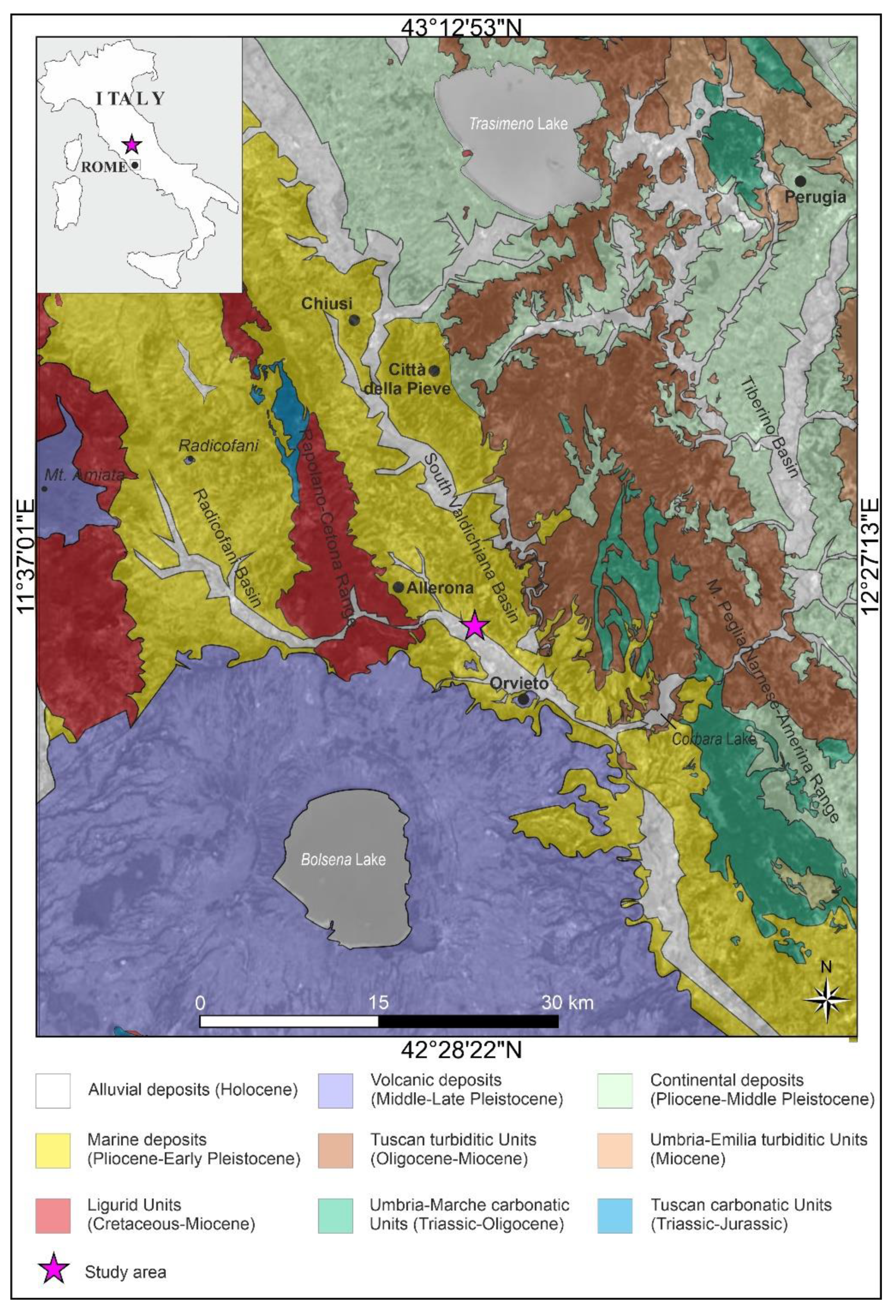
2. Geological Setting

The study area (Figure 1) pertains to the Miocene–Pleistocene South Valdichiana Basin [28], a NW–SE-oriented intermontane basin bounded by conjugated systems of extensional faults; it is part of the Neogene–Quaternary evolution of the Northern Apennines [29,30]. From the Pliocene onwards, the basin was filled with marine and continental deposits, and three main depositional cycles were recognised (Figure 2a; [28]):
-
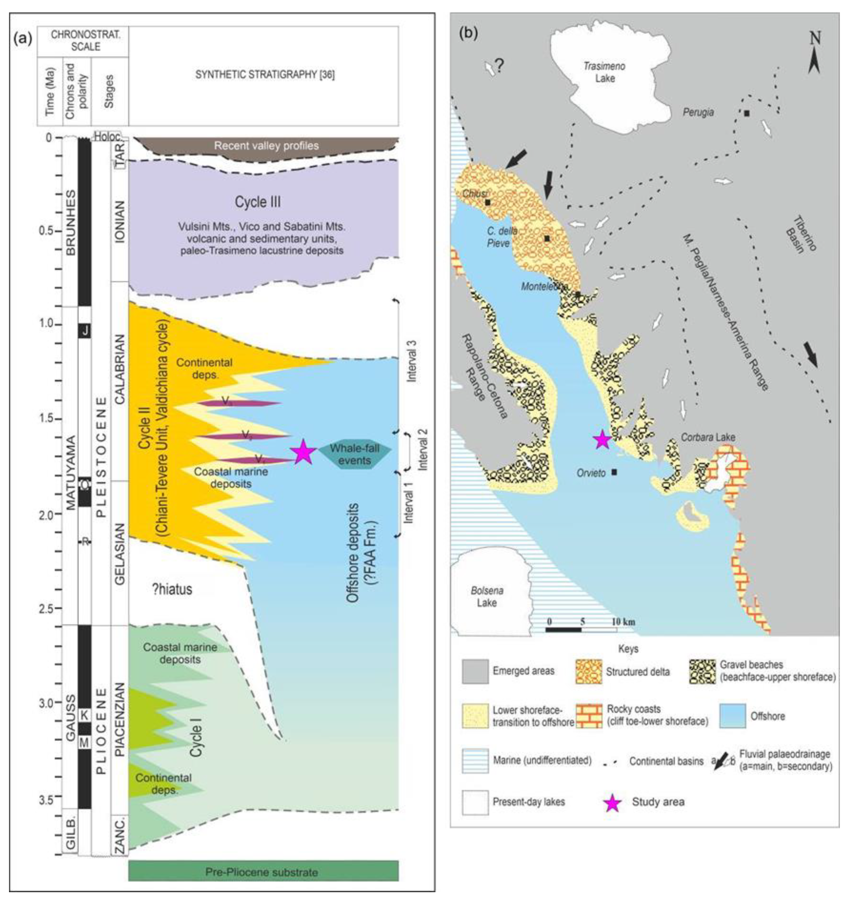
the “Pliocene” Cycle, widely documented in neighbouring basins [28,30,31], is suspected but not yet recognised in the study area. Although the deposits are age-equivalent to the FAA Fm (Formazione delle Argille Azzurre [28,31]), they are reported as Cycle I (Zanclean–Piacenzian hypothetic evolution of coastal areas) and offshore deposits (continuous/paraconformable distal marine sedimentation) [28].
-
the Valdichiana Cycle (Gelasian–Calabrian), mainly consisting of the Chiani–Tevere unit and encompassing the higher lateral facies heterotopy and paleoenvironmental complexity of the area (Figure 2b), varying (from north to south and from coastal areas to the inner basin) from alluvial plains, deltas, river-fed beaches, rocky coasts, and shallow marine areas (shoreface to offshore transition), to open marine areas (~120–150 m deep [32,33]). This cycle is divided into three intervals by means of an integrated event stratigraphy (Figure 2a), and they are dated to Gelasian p.p. (Interval 1), Gelasian p.p.–Calabrian p.p. (Interval 2), and Calabrian p.p. (Interval 3) [28].
-
the Middle–Late Pleistocene evolution (Cycle III [28]), which is mainly represented by Paleo–Trasimeno lacustrine deposits northwards and in the southern part of the basin by the volcanic and sedimentary units of the Vulsini Mts., Vico Mts., and Sabatini Mts. This latest cycle precedes the onset of the present-day valleys (Late Pleistocene–Holocene, Figure 2a).
Volcanic deposits of the Vulsini Mts. Are mainly characteristic of the third depositional cycle, from ~750 ka to ~330 ka [34]. Nonetheless, older deposits, still referred to as resulting from Vulsini activity [35], were found in both marine and continental deposits of the Valdichiana Cycle [28] and dated to 1.7–1.4 Ma (V1 to V3 in Figure 2a). Together with whale-fall events, they highlight Interval 2 in the Valdichiana Cycle (1.75–1.59 Ma [28]). This narrow sea strait and its northern termination in the gulf of Chiusi-Città della Pieve [28,36] were frequented by cetaceans during the Early Pleistocene at least, and the presence of at least three whale-fall events (Figure 2a) has already been documented [33,37,38].
The Holocene evolution of the area in a fluvial/alluvial environment was mainly driven by the presence of two major rivers, the Paglia River and the Tiber River, and by related processes (e.g., vertical and areal erosion, valley calibration, river capture, lateral shift of channels, flood episodes, and slope processes [39,40]).
Even though it has been significantly modified by anthropogenic activities, the Paglia River follows a complex path, from the southern slopes of Mt. Amiata to its confluence in the Tiber River, near the village of Baschi (Figure 1). Particularly in the study area, the actual riverbed cuts the Early Pleistocene marine clay sediments (Figure 3a [28,41,42]); at least one order of river terraces can be clearly recognised (Figure 3b,d). Although morphological evidence suggests a wider distribution (4 km or more in the NW–SE direction), mineralised structures were mainly found in a ~2 km narrow path along the Paglia River bends, a few kilometres north of the town of Orvieto (Figure 1 and Figure 2). The mineralised structures (Figure 4) partly emerged from the Early Pleistocene deposits where the November 2012 exceptional flooding event removed part of the covering alluvial deposits (Figure 3b,c).

3. Materials and Methods

Forty-two structures were described and measured in the field, and their positions were mapped by GPS (Table 1). On 8 different structures (i.e., the best-preserved and most complete), 14 samples were collected and processed for mineralogical, isotopic, and organic geochemical analyses. The sampling points for the 8 structures are detailed in Table 2 and Figure 4. Biostratigraphic and micropaleontological data were obtained for two samples (PAG 1 and PAG 2) of hosting clay sediments (collected just above structures #4 and #5) and 1 clay sample (PAG 3) collected outside of structure #14 (Figure 4i).
Table 1. Details of the morphology, sizes (diameters and heights), and GPS coordinates of the conduit concretions identified in the 2016 and 2017 surveys. Bold numbers indicate the analysed conduits.
Conduit
Concretions
MorphologyDiameters (Max, min)HeightCoordinates
1doughnut60 cm10 cm42°45′27.99″ N12°4′55.19″ E
2troncoconical30 cm20–25 cm42°45′27.69″ N12°4′55.72″ E
3doughnutM 68 cm;
m 55 cm
18 cm42°45′27.62″ N12°4′55.92″ E
4doughnutM 120 cm;
m 62 cm
30 cm42°45′27.27″ N12°4′56.11″ E
5troncoconicalM 78 cm;
m 60–76
30 cm42°45′27.04″ N12°4′56.65″ E
6troncoconicalM 107 cm;
m 92 cm
40 cm42°45′27.35″ N12°4′57.01″ E
7doughnutM 360 cm;
m 340 cm
80 cm42°45′26.93″ N12°4′58.22″ E
8troncoconical with 2 mouthsM 132 cm;
m 125 cm
72–73 cm42°45′26.56″ N12°4′57.77″ E
9troncoconicalnot measured/on the river flow 42°45′25.95″ N12°4′57.56″ E
10doughnutM 195 cm;
m 165 cm
85 cm42°45′25.89″ N12°4′58.50″ E
11doughnutnot measured/on the river flownot measured42°45′25.37″ N12°4′57.97″ E
12stacked doughnutM 380 cm;
m 330 cm
not measured42°45′25.46″ N12°4′58.58″ E
13troncoconical with two mouthsM 190 cm;
m 90 cm
75 cm42°45′25.75″ N12°4′58.73″ E
14ring doughnut with large central mouthM 185 cm;
m 170 cm
27 cm42°45′25.67″ N12°4′59.03″ E
15troncoconicalnot measured/on the river flow 42°45′25.07″ N12°4′58.79″ E
16ring doughnutM 190 cm;
m 190 cm
45 cm42°45′25.12″ N12°4′59.83″ E
17ring doughnutM 290 cm;
m 190 cm
70 cm42°45′24.81″ N12°4′59.89″ E
18troncoconical with central mouthM 80 cm;
m 72 cm
30 cm42°45′24.56″ N12°4′59.52″ E
19troncoconicalM 88 cm;
m 73 cm
24 cm42°45′24.65″ N12°5′0.26″ E
20 stacked doughnutM 200 cm;
m 170 cm
95 cm42°45′24.37″ N12°5′0.75″ E
21troncoconical irregularM 145 cm;
m 125 cm
3542°45′23.62″ N12°5′0.80″ E
22irregularon the river flow 42°45′23.59″ N12°5′0.65″ E
23stacked doughnut with central mouth and accessory small holesM 175 cm +50; m 175 cm65 cm42°45′23.48″ N12°5′1.23″ E
24troncoconical with two mouthsM 200 cm;
m 188 cm
50 (15 + 25 + 10)42°45′22.24″ N12°5′1.75″ E
25troncoconical with two mouthsM 95 cm;
m 25 cm
50 cm42°45′22.19″ N12°5′1.46″ E
26troncoconical with central mouthM 115 cm;
m 100 cm
60 cm42°45′22.13″ N12°5′1.36″ E
27doughnutM 240 cm;
m 180 cm
40 cm42°45′21.87″ N12°5′1.15″ E
28doughnutM 190 cm;
m 160 cm
50 cm42°45′21.36″ N12°5′2.28″ E
29stratiform
concretions
on the river flow 42°45′22.10″ N12°5′1.09″ E
30 to 33ellipticalon the river flow ??
34elliptical
spiralled
M 185 cm;
m 160 cm
15 cm42°45′15.85″ N12°5′16.05″ E
35elliptical
spiralled
M 200 cm;
m 137 cm
25–30 cm42°45′15.67″ N12°5′17.19″ E
36very large stacked doughnutnot measured on the opposite riverbank 42°45′15.31″ N12°5′17.29″ E
37crescent shapeon the river flow 42°45′15.63″ N12°5′17.54″ E
38stratiform
concretions
M 320 cm;
m 280 cm
135 cm42°45′15.51″ N12°5′17.66″ E
39crescent shapesubmerged 42°45′15.20″ N12°5′17.53″ E
40 and 41irregularsubmerged 42°45′15.52″ N12°5′17.98″ E
42ring doughnutM 60 cm;
m 20 cm
30 cm42°45′15.75″ N12°5′14.58″ E
Table 2. Position of sampling points from selected structures and morphologies.
SamplePositionStructure Morphology
5 topperiphery, upper surfacetroncoconical
5 bottomperiphery, ~40 cm below sample 5 top
5aclose to the mouth
5b10 cm from the mouth
8aclose to the mouth (a)troncoconical, with two mouths
8bclose to the mouth (b)
14periphery, upper ringring doughnut
17periphery, upper ringring doughnut
20periphery, upper ringstacked doughnut
24periphery, upper ringstacked doughnut
38 topupper surface, close to the mouthstratiform concretion
38 bottom60 cm below sample 38 top
42periphery, external ringring doughnut
42 rimrim around the mouth
For each clay sample, 100 g was immersed in a solution of water and 5% hydrogen peroxide for 48 h. These were then rinsed and filtered with a Satylon retina (63 micron mesh) to remove particles smaller than 63 microns. The residues were dried in an oven at 70 °C. All the structure samples were processed for thin section preparation and analysed under a polarised light microscope (Zeiss, Department of Physics and Geology, University of Perugia, Perugia, Italy).
The sample mineralogical compositions were investigated using an X-ray powders diffractometer (XRPD) Bruker D2 Phaser 2nd Generation, under the following experimental conditions: X-ray tube, copper (Cu) type; wavelength 1.5418 Å at 30 kV and 10 mA; scanned range 2θ, varying from 5° to 65°, at a scan speed of 5°/min in steps of 0.05°.
Back-scattered electron (BSE) imaging and supporting geochemical analyses were conducted at the Center for Instrument Sharing at the University of Pisa (CISUP) using an FEI Quanta 450 FEG-SEM equipped with a standardless EDS system using a Bruker Quantax 400—Xflash detector.
Stable isotope analyses were performed using a Gas Bench II (Thermo Scientific, Waltham, MA, USA) coupled to a Delta XP IRMS (Finnigan) at the Institute of Geosciences and Earth Resources at the Italian National Research Council (IGG-CNR) in Pisa. Carbonate samples of ca.0.15 mg were dissolved in H3PO4 for 5 h at 70 °C. All the results were reported relative to VPDB and VSMOW international standards. Sample results were corrected using the international standard NBS-18 and a set of three internal standards, previously calibrated using the international standards NBS-18 and NBS-19 and by laboratory intercomparisons. Analytical uncertainty for both δ18O and δ13C measurements was ±0.1‰.
For the organic geochemical analyses, sediments were extracted as dried ground powders first with cyclohexane (CH) and then with dichloromethane (DCM). CH extracts were examined directly for organic geochemical biomarker hydrocarbons of the anaerobic oxidation of methane (AOM) by gas chromatography (GC) methods, including GC, high-temperature GC (HTGC), GC–mass spectrometry (GC–MS) and HTGC–MS. DCM extracts were examined similarly for polar biomarkers of AOM, but this examination occurred after derivatisation with BSTFA (cf [5]). Finally, residues after CH and DCM extraction were methylated, and the methyl esters were also examined by the above GC methods. Detailed descriptions are provided in the Supplementary Material [43,44,45,46,47].

4. Results

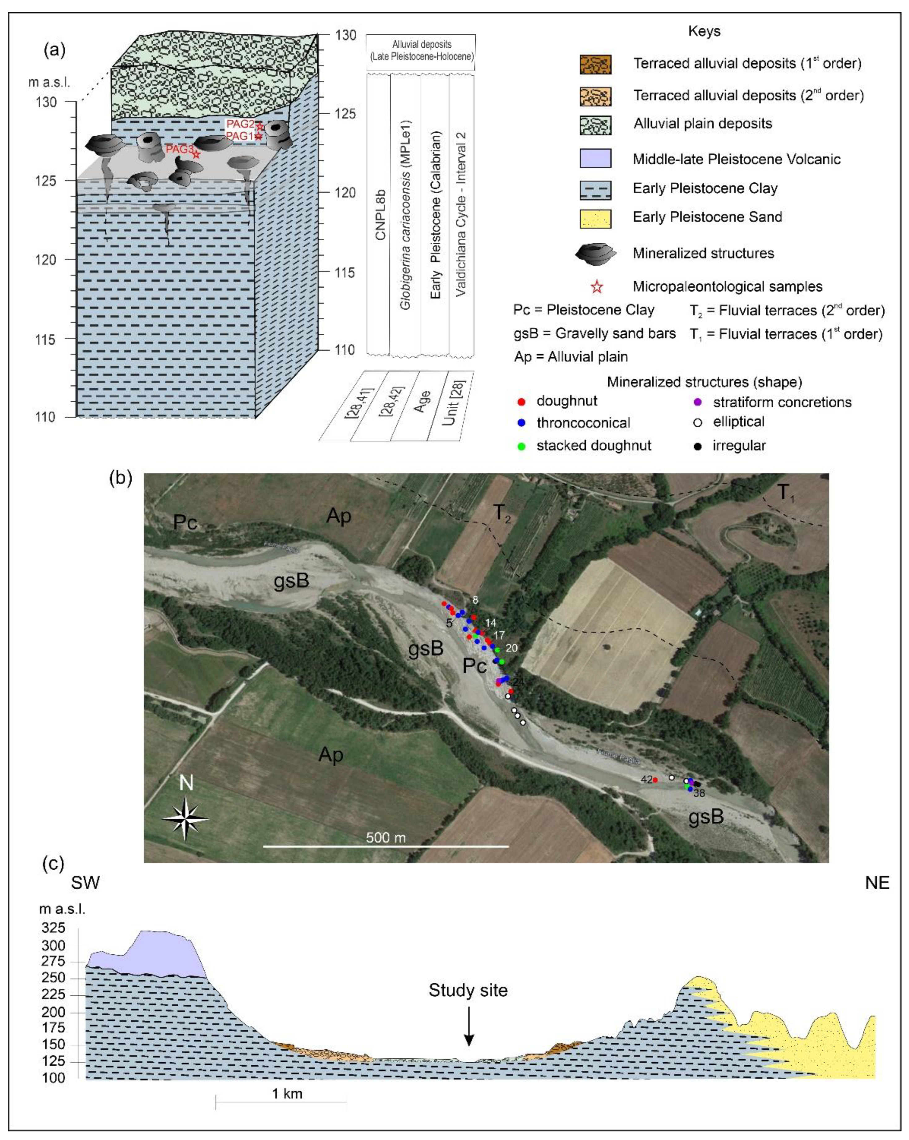
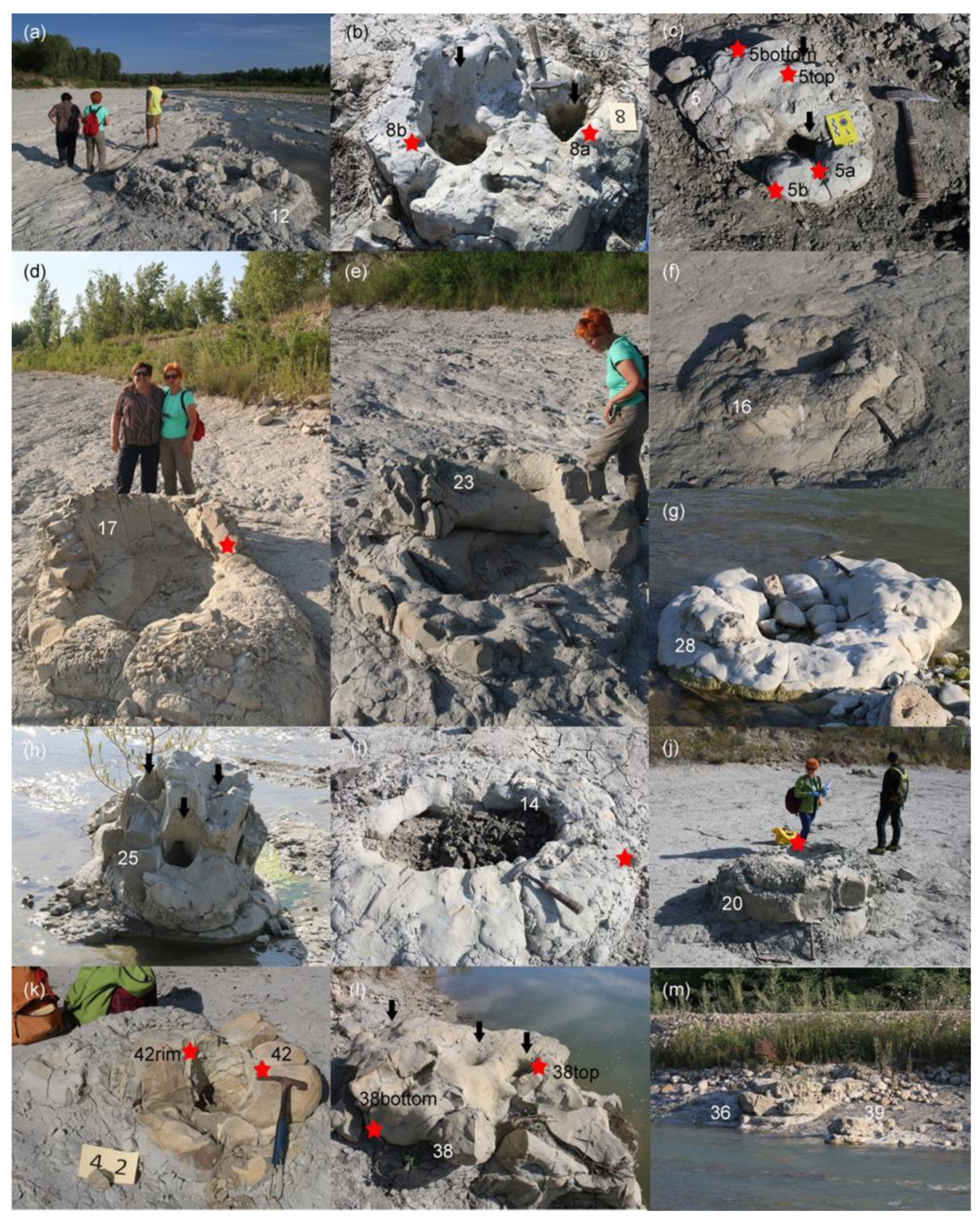
4.1. Conduit Concretion Morphology and Spatial Distribution

The conduit concretions (“all concretions possessing conduits”, sensu [2]) along the Paglia riverbed, which are also visible in the aerial photos from 2015 to 2019 (Figure 3b and Figure 4), were geolocated and measured directly in the field and the data are reported in Table 1.
Minimum/maximum diameters were slightly variable (Table 1), from 20 cm to more than 300 cm, with no clear relation between dimensions and morphologies.
The main common morphologies (following the nomenclature of [1,2]) were doughnuts (with two different shapes: ring doughnut and stacked doughnut) and troncoconicals (Figure 4). Locally stratiform concretions (sensu [2]) also occurred. The ring doughnuts (Figure 4d,f,g,i,k) were characterised by a single central mouth variable in size from 30 cm to over 150 cm. The larger elliptic specimen (Figure 4d) showed small circular openings (variable in size from 1 to 3 cm) placed in the inner portion of the wall. The stacked doughnuts (Figure 4a,e,j,m) were the largest and consisted of three or four perfectly stacked doughnuts, but these often showed partially preserved outlines. Additionally, in this case, small circular openings (Figure 4e) were visible in the inner portion of the walls. The troncoconical morphology was most common (Figure 4b,c,h) and possessed one or two open conduits (mouths), generally of similar diameters. The stratiform concretions (Figure 4l) were rarer and mainly emerged in the middle of the watercourse; they were massive and elongate and supported at least 10 openings with diameters variable from 1 cm to 25 cm. This morphology, according to [2], could represent the lateral coalescence of several conduits.

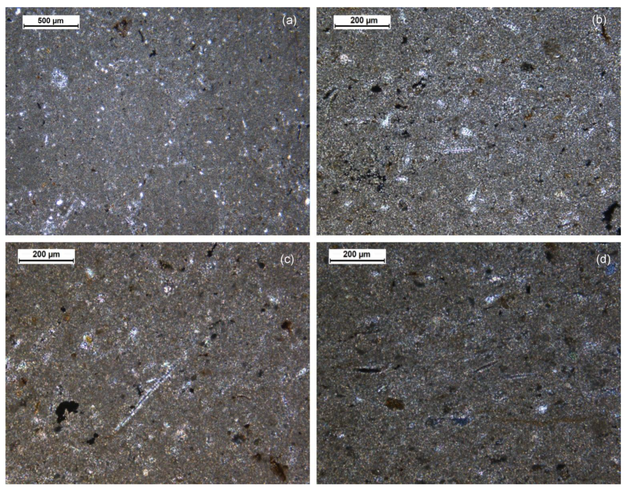
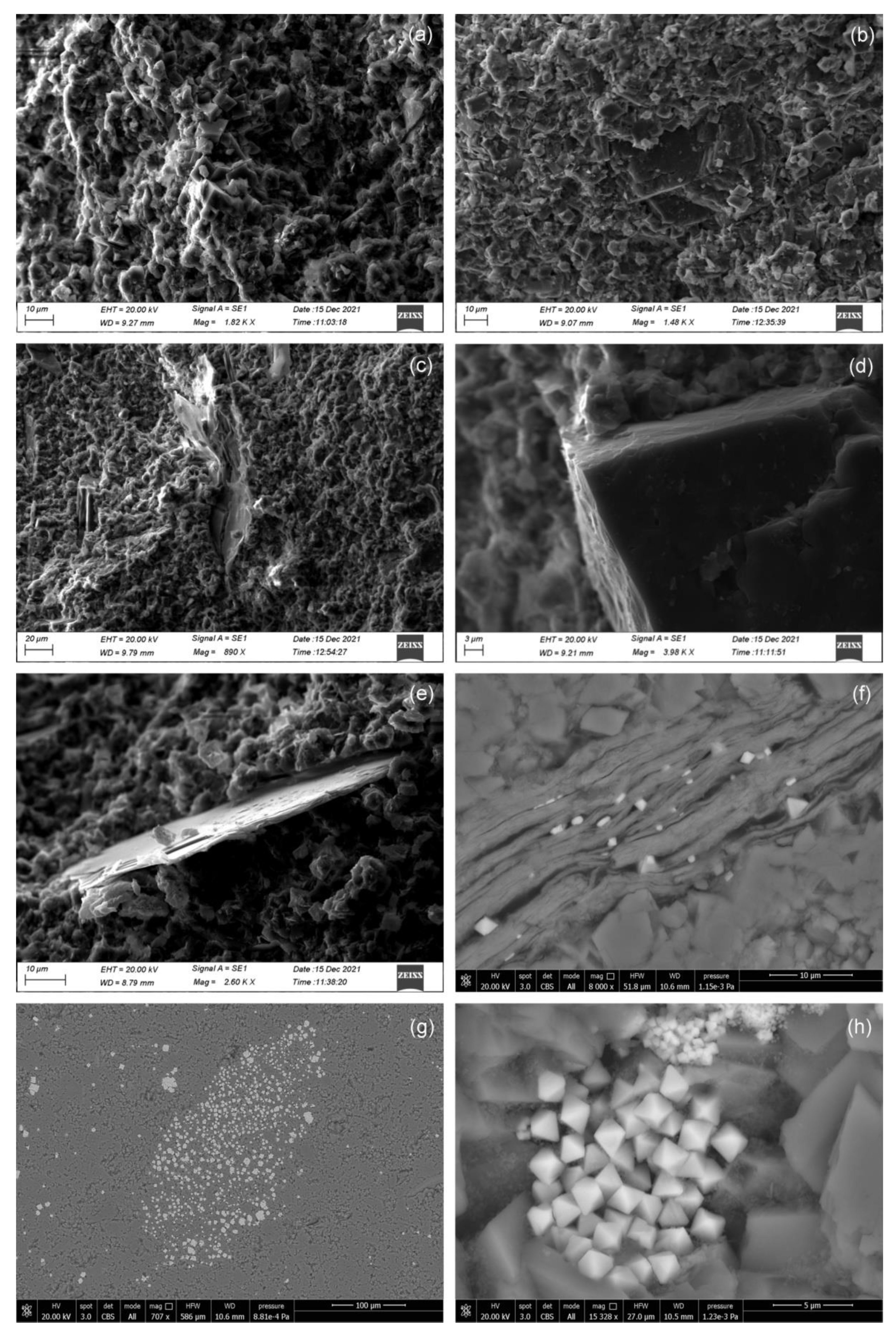
4.2. Mineralogical and Petrographic Features

Macroscopic observations in the field revealed that the conduit concretions were mainly light grey. Only two (structures 17 and 42, Figure 4d,k) were hazelnut in colour. The mouths of conduits were covered with a thin (from 1 mm to 2 mm), striated, smooth, light-yellow finish, which mineralogical analysis recognised as calcite.
Microscopic examinations of thin sections and XRPD analyses showed that the samples were composed of two types of matrixes: the first (structures 5 and 14) was represented by micropeloids (aggregates of about 1 mm or larger), composed of microcrystalline dolomite and rare micrite (Figure 5a–c). The second (structures 8, 17, 20, 24, 38, and 42) was a fine homogeneous matrix of dolomite microcrystals with common pyrite crystal aggregates (Figure 5d and Figure 6a) and randomly distributed filamentous structures with diameters up to 10 μm, and lengths variable from 40 to 200 μm (Figure 5c,d).
The detrital fraction always includes quartz in association with traces of feldspars, micas, kaolinite, apatite, and pyrite (Table 3).
SEM–EDS analyses revealed that the filamentous structures were represented by clay minerals completely enveloped by euhedral dolomite microcrystals (Figure 6c,f). The clay minerals commonly occurred, as did very fine silt-sized grains of quartz and plagioclase, as well as a few foraminifer tests filled by pyrite (Figure 5a). The very small size of the dolomite (from 2 to 25 μm) and the low porosity are indicative of a very high precipitation rate.
Table 3. Mineralogical composition determined by XRPD and SEM/EDS analyses, values of stable isotopes (13C, 18O), and Z value of the eight conduit concretions and minerals detected. Z is calculated according to Formula (1).
SamplesDolomiteCalciteQuartzPlagioclaseMicaKaoliniteApatitePyriteδ13Cδ18OZ
5 topXXXXXtrtrtrtrtr0.681.58129.47
5 bottomXXXtrXtrtrtrtrtr0.772.45130.09
5aXXX Xtrtrtrtrtr0.363.13129.59
5bXXX Xtrtrtrtrtr−0.413.44128.17
17XXX Xtrtrtrtrtr−0.574.07128.10
8aXXX Xtrtrtrtrtr1.452.89131.70
8bXXX Xtrtrtrtrtr2.303.13133.56
14XXX Xtrtrtrtrtr4.453.27138.04
20XXX Xtrtrtrtrtr4.793.66138.93
24XXX Xtrtrtrtrtr4.333.64137.98
38 topXXX Xtrtrtrtrtr3.603.39136.36
38 bottomXXX Xtrtrtrtrtr3.233.23135.52
42XXX Xtrtrtrtrtr2.463.67134.17
42 rimXXX Xtrtrtrtrtr4.053.01137.09
XXX = very abundant, X = present, tr = trace.

4.3. Organic Geochemical Biomarkers

Organic geochemical biomarkers of anaerobic methane oxidation (AOM) are well-known (e.g., [5,48]) and include the hydrocarbons crocetane [49] and pentamethylicosane (formerly known as pentamethyleicosane [50]), as well as the ether archaeol [51], all of which are likely biological products of archaea and related microbes [52]. The 13C isotopic values of these compounds are also often very distinctive (typically −150‰ [48]). Unfortunately, none of these compounds was detectable in any of the structures examined, despite the use of appropriate methods.
Indeed, the amounts of extractable organic matter in the samples were very low (typically 0.1–0.5 mg per 5 g sample, with 0.1 mg in the blank). The hydrocarbons and other more polar compounds that were detected were mainly atypical of indigenous material. For example, sterane and triterpane biomarkers showed distributions mainly typical of mature petroleum, unexpected in Pleistocene sediments (c.f., the immature distributions found by [5] in Miocene deposits in New Zealand). Although other commonly used biomarker parameter estimates (e.g., Carbon Preference Index, CPI; Odd over Even Preference, OEP; and Average Chain Length, ACL of n-alkanes; Tables S1 and S2) varied according to the method of calculation; nonetheless, CPI values around 1.0 were typical (Table S2). These also indicated the presence of thermally mature hydrocarbons, as did the presence of unresolved complex mixtures of hydrocarbons [53]. Squalene was also present in most hydrocarbon extracts but is not diagnostic and may be an artefact; phthalate esters, which are common plasticisers, were also identified in the more polar fractions [54].

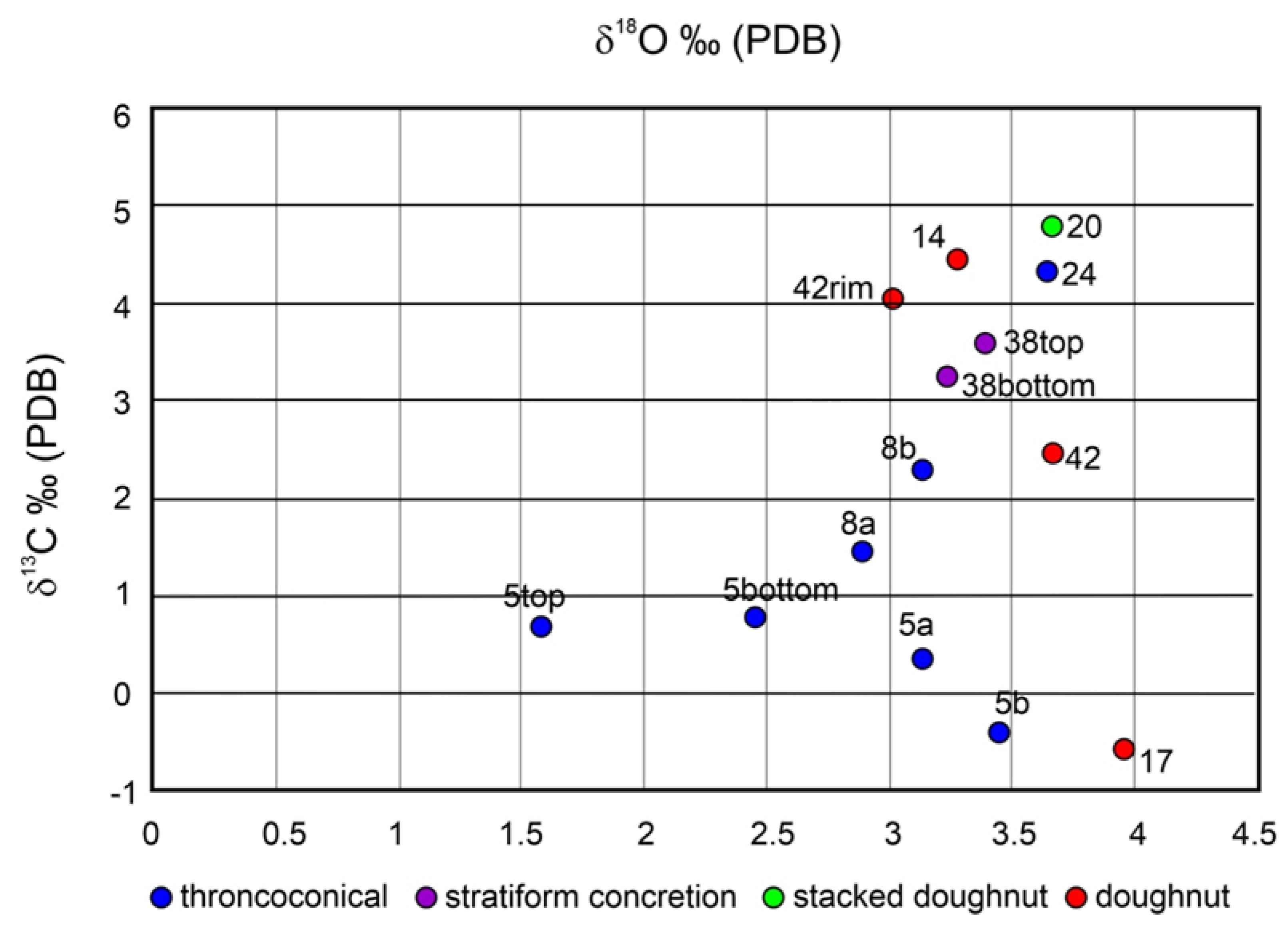
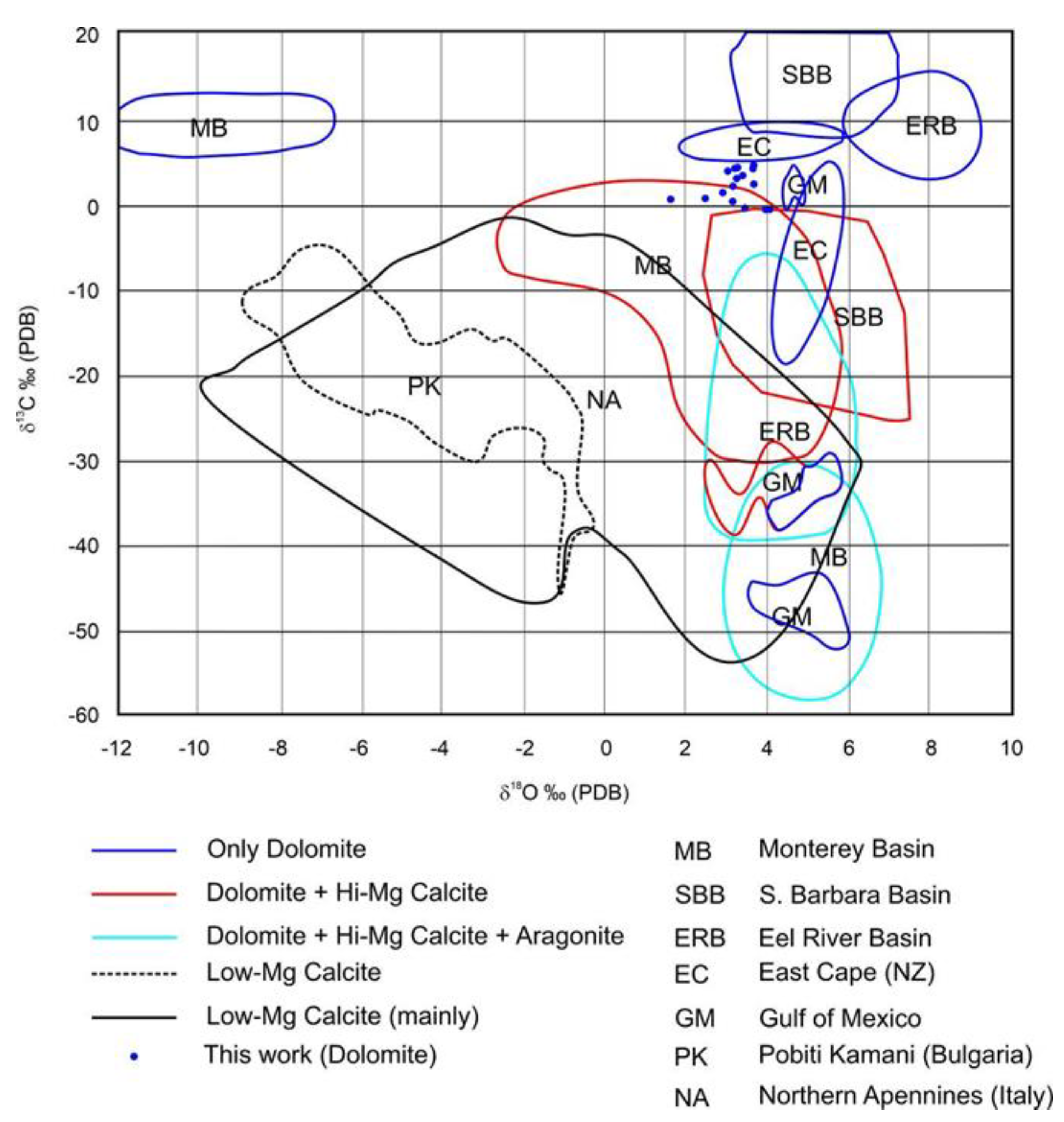
4.4. Stable Isotopes

The isotopic compositions of carbon and oxygen in the carbonates may indicate the conditions under which they formed. The 13C ratio values indicate the carbon sources that may have participated during carbonate formation (biogenic, abiogenic, or thermogenic methane, or their mixtures). The 18O ratio values allow for the determination of the pore water temperatures in which carbonate minerals precipitate. In addition, C–O stable isotope values could be useful for evaluations of the paleo-salinity of the water and can be inferred from the Z value [55], calculated according to the formula:
Z = 2.048(δ13C + 50) + 0.498(δ18O + 50)
If Z < 120, this indicates a freshwater environment; if Z > 120, this indicates a marine environment or the participation of seawater during precipitation.
δ13C values of the bulk concretionary carbonate (dolomite) in this study ranged from −0.57 to +4.79‰ PDB (average + 2.22‰). δ18O values ranged from +1.58 to +4.07‰ PDB (average +3.23‰; Table 3). The Z values of the samples were higher than 120, which indicates the influence of seawater in providing the Mg2+ source for the formation of the dolomite.
There is no clear trend in the isotope values from the centre or the rim of the dolomite-rich conduits, suggesting an erratic precipitation.

4.5. Hosting Sediments

The clay deposits containing the conduit concretion field were dated to Early Pleistocene and associated with Interval II in the Valdichiana Cycle [28].
The grey clay marine deposits, occurring in a small outcrop (50 cm in thickness) above the conduit concretion surfaces (samples PAG 1 and PAG 2) and a few centimetres next to structure #14 (sample PAG3), were treated to obtain washed residues for micropaleontological analyses. The washed residues (~1 g) of samples PAG 1 and 2 contained moderate to rich assemblages of microfossils represented by benthic and planktonic foraminifers and very few fragments of bivalves or small carbonised wood fragments. The planktonic foraminifers were represented by the common Orbulina universa and the rarer Globorotalia inflata, Globigerina cariacoensis, and Turborotalita quinqueloba in assemblage with Globigerinoides ruber and Globigerinoides sacculifer. The benthic foraminifers were represented by both epifaunal and shallow infaunal species. The detritivores Lenticulina calcar and Siphotextularia concava and the herbivorous Cibicidoides lobatulus were abundant among the epifauna, and Nonionella turgida and Vaginulina striatissima were abundant among the shallow infauna. Hyalinea balthica was rare but always present in assemblages. In particular, the occurrence of H. balthica indicates a bottom temperature ranging between 4 and 12 °C [56]. The occurrence of L. calcar and H. balthica, both inhabitants of cold water, indicates that the sea floor was cool and the sediment rich in organic matter (or phytodetritus). This last factor is evidenced by the abundance of the species S. concava and N. turgida, which prefer sediments rich in organic matter but do not tolerate high organic fluxes [37]. Moreover, the occurrence of shallow infaunal benthic species (V. striatissima, N. turgida, and H. balthica) indicates normal oxygenation at the water–sediment interface, and the abundance of epiphytal and herbivorous C. lobatulus suggests the existence of a sea grass prairie.
The assemblage of sample PAG3, collected next to structure 14 (stratigraphically below sample PAG1), was quite different, with a decrease in planktonic species, represented only by the common O. universa and the very rare Globigerina bulloides, G. cariacoensis, and G. ruber, all affected by pyritisation. The benthos were enriched with the entrance of shallow infaunal species such as Marginulina costata and Bigenerina nodosaria; that added up to very abundant L. calcar and N. turgida.

5. Discussion

5.1. Origin of the Fluids

Dolomite commonly makes up only a small percentage of seep carbonate lithologies, but sometimes—as in the present work—it is the dominant mineralogy. Its formation and distribution are often ambiguous. Most authors report the occurrence of seep-related dolomite as strictly related to low-temperature microbially mediated reactions in the shallow subsea floor ([57] and references therein).
In particular, in methane seeps, the anaerobic consumption of seawater sulphate by consortia of archaea and sulphate-reducing bacteria causes a depletion in MgSO4 and is accompanied by an increase in the concentration of free Mg ions and an increase in pore water alkalinity and eventual HCO3 supersaturation, thereby favouring the preferential formation of dolomite [2].
However, most microbially mediated low-temperature primary dolomite formation that directly precipitates is characterised by organic biomarkers and negative δ13C values, as reported in Figure 7 and Figure 8.
Our studies indicate a mineralogical composition of the conduits dominated by microcrystalline euhedral dolomite, with minor plagioclase, mica, kaolinite, quartz, very few foraminifers, and with no, or rare, organic material.
This evidence, together with the positive values of δ13C and the absence of organic geochemical biomarkers of anaerobic methane oxidation (AOM), may suggest an unusual, inorganic origin for the seep conduits, unrelated to microbially mediated reactions.
The positive δ13C values can be compared with those found in some East Cape dolomite concretions (δ13C +6 to +9‰ vs. PDB) [2] (Figure 8) and interpreted as sourced from reduced CO2 as a by-product of methanogenesis and derived from the microbial production of methane during a shallow burial (10–100 m) of the sediment pile. The East Cape concretion-related biomarkers confirmed that AOM by methanotrophic archaea and sulphate-reducing bacteria occurred in the sediments [5], even though the δ13C values of the carbonate cements are dominantly positive [2].
However, the absence of organic geochemical biomarkers of anaerobic methane oxidation (AOM) in our dolomite concretions seems to exclude this possibility. The other remaining possible origin explaining the observed δ13C values is the direct emission of hydrothermal/volcanic carbon dioxide.
In the study area, the inorganic origin of CO2-rich fluids is probably related to a process of CO2 diffusion degassing associated with volcanic activity starting from the Early Pleistocene (about 1.7 Ma) [59].
The δ13C values of carbonates, ranging from −0.57 to +4.79‰ vs. PDB, are consistent with a magmatic origin of the gas phase. The fluids released by Italian volcanoes and geothermal regions are characterised by δ13C values of the original gas phase (before dilution or fractionation) between −3 and −1‰ vs. PDB (e.g., [60,61,62]). Similar values are also computed by [63], to explain the isotopic evolution of Vesuvio groundwaters, while the δ13C values of the Campanian submarine gas emissions range from −1.8 to −2.3‰ vs. PDB.
Starting from this range of δ13C values for the deep gas phase, we suggest that the more positive carbon isotopic composition of our solid samples is explained by the fractionation that occurred during the degassing and subsequent carbonate precipitation phases at low temperature, which can lead to a positive isotopic shift of some delta units [63]. The accurate value of the isotopic shift cannot be calculated for our samples because it depends on the pressure at which degassing occurred and the possibility of a multiple-step degassing process. As an example only, [63] calculated an isotopic shift of about +4 delta units from the continuous degassing of a saturated 24-bar CO2 solution brought to a pressure of 1 bar.
Oxygen isotope values recorded in the carbonate samples relate mainly to the fluid composition at the time of carbonate precipitation and the temperature of precipitation.
Considering that the δ18O values of our samples range between 1.58 and 4.07‰ vs. PDB (Table 3 and Figure 7) and assuming the present seawater δ18O (0‰ SMOW), the calculated temperature of precipitation, following the fractionation factor of [64], ranges from 20 to 30 °C.
In contrast, the benthic epifaunal and shallow infaunal foraminifers present in the hosting sediments indicate that the temperature at the bottom was low, specifically, in the range between 4 and 12 °C, marking permanent cold bottom water conditions and a cold overlying water column.
In order to explain the temperature of dolomite precipitation inferred from the oxygen isotope values, we propose that warm, CO2-rich fluids rose through the carbonate conduits and mixed with this cold seawater.

5.2. Formation of Dolomite Conduits

The large dolomite-rich doughnut concretions were associated by [2] with intermittent fluid ascent (CO2 in the present case), where fluid periodically becomes trapped by relatively more impervious (perhaps clay-enriched) stratigraphic layers. The authors of [6] suggested that seep-related tubular (conduit) concretion formation occurred in the subsurface, from cement precipitation, starting at the outer rims of concretions and continuing toward the centre of their conduits.
In our case, the centre of each structure is very open (as shown in Figure 4), unlike those reported by [2,6], which had completely filled central areas (mouths).
The free and well-formed mouths, covered with a thin (from 1 mm to 2 mm) calcitic patina with longitudinal striae (Figure 4b,i,h,l), underline the rise of a vertical flow under pressure (presumably a mixture of gas and liquid).
The calcite crystals were also found near the small (centimetre) mouths distributed along the internal rims of the doughnut structures (Figure 4e,l).

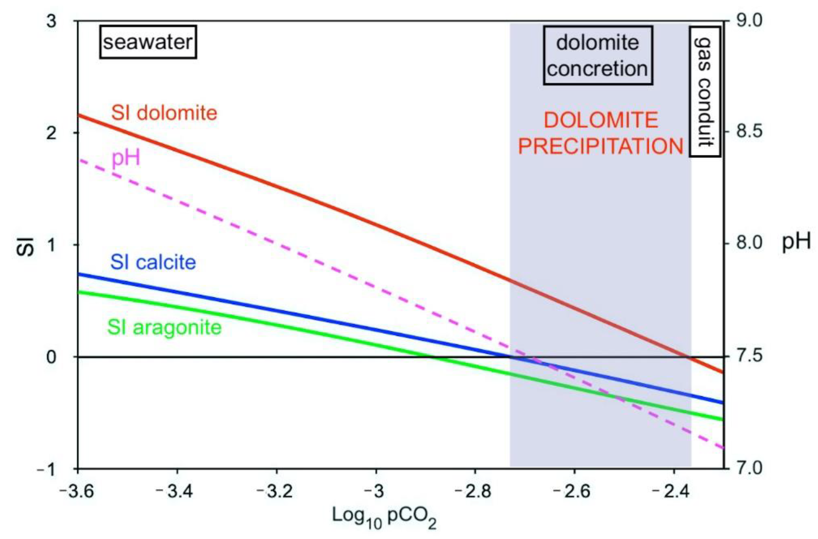
5.3. CO2 Flux and Dolomite Stability

In order to explain the ubiquitous occurrence of dolomite in the carbonate conduits, it is necessary to investigate the influence of CO2 on the stability of the carbonate mineral species. The presence in the study area of an Early Pleistocene volcanic degassing zone is suggested by the occurrence of distal pyroclastic-fallout materials in the marine clay sediments [28,34,59]. These deposits, with ages between 1.75 and 1.2 Ma, have a local origin, probably from a small eruptive centre near Orvieto. Considering the composition of the volcanic products, it is likely that the degassed phase was very similar to the gas emitted in the present day from Latera and Torre Alfina, located a few kilometres south of the study area, and by the CO2-rich springs of Parrano and Monte Rubiaglio (Figure 9, [65,66,67,68]).
If the degassing process occurred in a relatively shallow marine environment, the volcanic CO2 seepage could have produced high values of CO2 partial pressure (pCO2) and the acidification of seawater, with the consequent undersaturation in calcite and aragonite, similar to that which is currently observed in present-day submarine volcanic hydrothermal fields [69].
In order to describe the possible interactions of the gas phase with seawater and with carbonate minerals, a theoretical water–gas–rock interaction model was constructed, starting with 1 kg of average seawater with a salinity of 35 ppt [70] and increasing the CO2 concentration from 0.02% to 0.5% in 96 steps at 10 °C. At each step, the saturation indexes (SI) of calcite, aragonite, and dolomite, along with pH and pCO2, were computed with the PHREEQC code [71,72] using the LLNL (Lawrence Livermore National Laboratory) thermodynamic database [73].
The results of the calculations (Figure 10) show that for pCO2 values normally found in shallow seawater, the solution is supersaturated in calcite, aragonite, and dolomite. In these conditions, even if dolomite had an SI higher than calcite, the formation of calcite would predominate over dolomite because of the relatively slow rates at which dolomite forms [67]. For increasing values of pCO2, the pH of the solution and the SI values of all the carbonate species decrease. At pCO2 values higher than 10−2.75 bar, the solution is undersaturated in calcite and aragonite but is still oversaturated in dolomite. In these conditions, the only carbonate mineral that can precipitate is dolomite. For pCO2 values higher than 10−2.35, dolomite is also undersaturated, and no carbonate mineral is allowed to precipitate.
According to the proposed geochemical model, the presence of CO2 seeps could produce, at the sediment–water interface, a narrow region around the gas conduit characterised by 7.5 > pH > 7.1 where dolomite precipitation is possible. For lower pH values, corresponding to pCO2 > 10−2.3, dolomite precipitation is thermodynamically not permitted, keeping the gas conduit open and allowing the progressive growth of the chimneys.

5.4. Effects of CO2 Flow in the Marine Environment and Inhabitants

Recently, the geochemical aspects of shallow marine CO2-rich seeps worldwide have been reviewed [69], focusing on both gas composition and water chemistry. The authors of [69] describe the geochemical effects of volcanic CO2 seepage on the overlying seawater column. In the CO2 seep sites off Vulcano Island (Sicily), in areas of intense bubbling, extremely high levels of pCO2 (>10,000 μatm) result in low seawater pH (<6) and the undersaturation of aragonite and calcite in an area devoid of calcified organisms such as shelled molluscs and hard corals. Around 100–400 m away from the Vulcano seeps, the geochemistry of the seawater becomes analogous to future ocean acidification conditions, with dissolved carbon dioxide levels falling from 900 to 420 μatm as seawater pH rises from 7.6 to 8.0 [74].
In this case study, the direct effect of CO2 emissions on the sea bottom seems to be restricted to the neighbouring area of the carbonate conduits. In fact, evidence of acidification at the water–sediment interface is highlighted by the decrease in the abundance of microfauna (mainly benthic foraminifers) in sediments close to the conduits.
The indirect effect of CO2 diffused (or trapped) in the clay sediments seems to be responsible for the acidification of interstitial (pore) water and the dissolution of calcitic bivalve shells (i.e., Megaxinus incrassatus) recovered as internal moulds in the carbonate conduits.
CO2 added to seawater changes the hydrogen ion concentration (pH); this may affect marine life through mechanisms that do not directly involve CO2. At high CO2 concentrations, animals can asphyxiate because their blood cannot transport enough oxygen to support metabolic functions. In the most active open ocean squid (Illex ilecerebrosus), model calculations predict acute lethal effects with a rise in pCO2 of 6500 ppm and a 0.25 unit drop in blood pH. However, acute CO2 sensitivity varies between squid species. It should be emphasised that squid are one of the main prey species of the sperm whale and some other toothed cetaceans [74].
However, direct effects of dissolved CO2 on diving marine air breathers (mammals and turtles) can likely be excluded since they possess higher pCO2 values in their body fluids than water breathers and gas exchange is minimised during diving. It is possible to speculate that marine mammals, such as sperm whales, may be indirectly affected through potential CO2 effects on their preferred food, the squid.

5.5. Geological and Palaeoenvironmental Implications

Although no evidence of pervasive fracturing was noted in the field, observations from satellite images indicate the alignment of isolated structures throughout the riverbed, suggesting that their distribution is controlled by faulting (Figure 3b and Figure 9). This alignment ranges between WNW and NW, and it is compatible with both the main trend of the basin (Figure 9) and the systems of fracture affecting the same clay in the Bargiano area [33,37,38]. This feature is well known and has been reported by several other researchers [2,75,76]. Although not conclusive, the presence of the study structure adds a new piece of evidence for reconstruction of the early Pleistocene tectonic and volcanic scenario. These vast fields of carbonate conduit concretions imply new considerations regarding the importance of hydrothermal CO2 emissions during the Early Pleistocene in southwestern Umbria and evidence the existence of tectonic activity and volcanic phenomena during this interval of time (Figure 9). Moreover, both CO2-related structures and whale-fall events (WFE) in the area are coeval with volcanic phase V1 (Figure 2a; [28,34,59]); the presence of other, as yet undocumented, fields of mineralised structures in the area cannot be excluded.
The presence of this CO2 degassing field and the emergence of volcanoclastic deposits [28,34,59] fits well with the local pattern of extensional faults (Figure 9). Such a situation is comparable with present-day CO2 emissions and CO2-rich springs [65] and is further evidence of the incipient volcanic activity of Mt. Vulsini since the Early Pleistocene. This phase was reasonably characterised by diffused, mainly submarine fissural activity, producing a dispersed pyroclastic fallout [59]. In this scenario, the occurrence of extensional faults also guided the rise of CO2 to the surface and their trapment in clay sediments at shallow depths below the sea floor (Figure 11). In this tectonically active context, the presence of the described mineralised structures was related to the progressive onset of escape paths followed by hydrothermal/volcanic CO2-rich fluids. This slow and progressive rise of fluids can justify both the almost exclusive presence of dolomite and the occurrence of thin calcite mineralisation only in the internal wall and in the mouths of conduits. According with [2], it is presumed that mineralisation took place at very shallow depths inside the sediment (i.e., just below the sea floor), with free gas emission at the water–sediment interface. The proposed model [2], linking mineralisation to fault systems, accounts well for the formation of large, multiple doughnut structures, and it is certainly applicable to this case study. Nonetheless, the relation with faulting seems to be here more generalised and related to a diffuse stress field rather than to main fault plains (i.e., the master faults bordering the basin, Figure 11). In fact, the accompanying volcanism progressively shifted southwestwards, during the Middle–Late Pleistocene (~750–100 ka), to the main area of the Vulsini Mts. (Figure 1 and Figure 2).
The possible effects of CO2 release in water on marine species have been discussed in Section 5.4. As shown in Figure 2 and Figure 8, the spatial and temporal localisation of WFE is still compatible with the tectonic context, although a direct correlation with the presence of CO2 in water is hardly justifiable. The high concentration of WFE in a restricted area still lacks a definitive interpretation [33,37,38]. The documentation of CO2-degassing carbonate conduits not far from the sites of WFE adds another piece to the paleoenvironmental puzzle, particularly to the hypothesis that their presence was more widespread than that documented previously. In this way, the paleoenvironmental correlation, whilst still feasible, is more nuanced. At this stage, it is only possible to infer that tectonics and volcanism guided the onset of paleoenvironmental conditions favourable to the presence of great cetaceans and were indirectly responsible for mass-death events, acting on parameters that somehow influenced the food chain.

6. Conclusions

This study reports the first occurrence of carbonate conduits made of dolomite of abiogenic origin in the clay marine deposits of the early Pleistocene. The morphological features of the conduits, the positive isotopic values of carbon and oxygen in the carbonates, and the thermodynamic considerations regarding dolomite stability suggest that dolomite precipitation was related to the rise of hydrothermal/volcanic CO2-rich fluids. This is in agreement with the early Pleistocene volcanic activity of the nearby Vulsini complex. The rising fluids were trapped inside the highly impermeable clay sediments until internal pressure reached the value of lithostatic pressure and broke the resistance of the hosting sediments, moving towards the seafloor. During their ascent, the hydrothermal/volcanic fluids mixed, at variable depths, with the seawater contained in the clay sediments, precipitating dolomite. The spatial distribution of the conduits clearly indicates that the fluid ascent followed preferential pathways corresponding to visible fractures related to early Pleistocene faults.

Supplementary Materials

The following supporting information can be downloaded at: https://www.mdpi.com/article/10.3390/min12070819/s1, Table S1: Gravimetric data from the cyclohexane (CH) and dichloromethane (DCM) extraction of carbonate conduit concretion samples and the extraction of esters following methyl esterification. Table S2: Calculated biomarker parameters. Figure S1: HTGC chromatograms of in-house nC10–30,40,50,60 alkanes standard, and cyclohexane extracts from procedural blank and carbonate conduit concretion. Figure S2: HTGC-ToF-MS (12 eV) total ion chromatograms of the cyclohexane extracts of the procedural blank and carbonate conduit concretions. Figure S3: HTGC-ToF-MS (12 eV) extracted ion chromatograms (m/z 136) of the cyclohexane extracts of the procedural blank and carbonate conduit concretions. Figure S4a: HTGC-ToF-MS (12 eV) extracted ion chromatograms (m/z 476) of the cyclohexane extracts of the procedural blank and carbonate conduit concretions. Figure S4b: Zoomed region HTGC-ToF-MS (12 eV) extracted ion chromatograms (m/z 476) of the cyclohexane extracts of the procedural blank and carbonate conduit concretions. Figure S5a: 12 eV mass spectrum of peak at 10.81 min. Figure S5b: NIST library mass spectrum (70 eV) of squalene. Figure S6: Mass spectrum of peak I at 13.51 min. Figure S7: Mass spectrum of peak II at 13.70 min. Figure S8: Mass spectrum of peak at 13.89 min. Figure S9: Peak area ratios using m/z 476 extracted ions for peak II/peak I and for peak III/peak I. Figure S10: HTGC-MS extracted ion chromatograms (upper m/z 191; lower m/z 217) indicating distribution of triterpanes and sterane biomarkers in sample 2. Figure S11: HTGC chromatograms of in-house nC10–30,40,50,60n-alkanes standard, and dichloromethane extracts of residues following cyclohexane extraction from procedural blank and carbonate conduit concretions. Figure S12: HTGC chromatograms of in-house C8-20n-fatty acid methyl esters (n-FAMEs) standard, and cyclohexane (methyl ester) extracts of residues following cyclohexane and dichloromethane extraction from procedural blank and carbonate conduit concretions.

Author Contributions

Conceptualisation, A.B., R.B. and F.F.; methodology, A.B., R.B., C.B., F.F. (Francesco Frondini), M.L., S.R. and P.A.S.; formal analysis, C.B., F.F. (Francesco Frondini), M.L., S.R. and P.A.S.; investigation, A.B., R.B., C.B., F.F. (Francesco Frondini), F.F. (Federico Famiani), M.L., S.R. and P.A.S.; writing—original draft preparation, A.B., R.B., C.B., F.F. (Francesco Frondini), M.L., S.R. and P.A.S.; writing—review and editing, All authors; visualisation, A.B., R.B., C.B., F.F. (Francesco Frondini), M.L., S.R. and P.A.S.; funding acquisition, A.B. All authors have read and agreed to the published version of the manuscript.

Funding

This research was funded by A.B. research funds (RICVABALDA).

Acknowledgments

We want to thank Ermindo Tardiolo, a connoisseur of the territory of Allerona, who first pointed out to us the existence of these structures emerging along the bed of the Paglia River; without his contribution, we would never have been able to study this particular topic. We also want to thank the three anonymous reviewers who contributed to the improvement of the initial manuscript.

Conflicts of Interest

The authors declare no conflict of interest.

References

  1. Capozzi, R.; Negri, A.; Reitner, J.; Taviani, M. Carbonate conduits linked to hydrocarbon-enriched fluid escape. Mar. Petrol. Geol. 2015, 66, 497–500. [Google Scholar] [CrossRef]
  2. Nelson, C.S.; Nyman, S.L.; Campbell, K.A.; Rowland, J.R. Influence of faulting on the distribution and development of cold seep-related dolomitic conduit concretions at East Cape, New Zealand. N. Z. J. Geol. Geop. 2017, 60, 478–496. [Google Scholar] [CrossRef]
  3. Judd, A.G.; Hovland, M. Seabed Fluid Flow—The Impact on Geology, Biology and the Marine Environment; Cambridge University Press: Cambridge, UK, 2007; pp. 1–475. [Google Scholar]
  4. Aloisi, G.; Pierre, C.; Rouchy, J.-M.; Foucher, J.-P.; Woodside, J. Methane-related authigenic carbonates of eastern Mediterranean Sea mud volcanoes and their possible relation to gas hydrate destabilisation. Earth Planet. Sci. Lett. 2000, 184, 321–338. [Google Scholar] [CrossRef]
  5. Pearson, M.J.; Grosjean, E.; Nelson, C.S.; Nyman, S.L.; Logan, G.A. Tubular concretions in New Zealand petroliferous basins: Lipid biomarker evidence for mineralisation around proposed Miocene hydrocarbon seep conduits. J. Petrol. Geol. 2010, 33, 205–220. [Google Scholar] [CrossRef]
  6. Nyman, S.L.; Nelson, C.S.; Campbell, K.A. Miocene tubular concretions in East Coast Basin, New Zealand: Analogue for the subsurface plumbing of cold seeps. Mar. Geol. 2010, 272, 319–336. [Google Scholar] [CrossRef]
  7. Campbell, K.A.; Francis, D.A.; Collins, M.; Gregory, M.R.; Nelson, C.S.; Greinert, J.; Aharon, P. Hydrocarbon seep-carbonates of a Miocene forearc (East Coast Basin), North Island, New Zealand. Sediment. Geol. 2008, 204, 83–105. [Google Scholar] [CrossRef]
  8. Metz, C.L. Tectonic controls on the genesis and distribution of late cretaceous, western interior basin hydrocarbon-seep mounds (tepee buttes) of North America. J. Geol. 2010, 118, 201–213. [Google Scholar] [CrossRef]
  9. Majima, R.; Nobuhara, T.; Kitazaki, T. Review of fossil chemosynthetic assemblages in Japan. Palaeogeogr. Palaeoclimatol. Palaeoecol. 2005, 227, 86–123. [Google Scholar] [CrossRef]
  10. Bojanowski, M.U. Oligocene cold-seep carbonates from the Carpathyans and their inferred relation to gas hydrates. Facies 2007, 53, 347–360. [Google Scholar] [CrossRef]
  11. Angeletti, L.; Canese, S.; Franchi, F.; Montagna, P.; Reitner, J.; Walliser, E.O.; Taviani, M. The “chimney forest” of the deep Montenegrin margin, South-Eastern Adriatic Sea. Mar. Petrol. Geol. 2015, 66, 542–554. [Google Scholar] [CrossRef]
  12. De Boever, E.; Swennen, R.; Dimitrov, L. Lower Eocene carbonate cemented chimneys (Varna, NE Bulgaria): Formation mechanisms and the (a)biological mediation of chimney growth? Sediment. Geol. 2006, 185, 159–173. [Google Scholar] [CrossRef]
  13. De Boever, E.; Huysmans, M.; Muchez, P.; Dimitrov, L.; Swennen, R. Controlling factors on the morphology and spatial distribution of methane-related tubular—Case study of an early Eocene seep system. Mar. Petrol. Geol. 2009, 26, 1580–1591. [Google Scholar] [CrossRef]
  14. Böttner, C.; Callow, B.J.; Schramm, B.; Gross, F.; Geersen, J.; Schmidt, M.; Vasilev, A.; Petsinski, P.; Berndt, C. Focused methane migration formed pipe structures in permeable sandstones: Insights from uncrewed aerial vehicle-based digital outcrop analysis in Varna, Bulgaria. Sedimentology 2021, 68, 2765–2782. [Google Scholar] [CrossRef]
  15. Conti, S.; Argentino, C.; Fioroni, C.; Salocchi, A.C.; Fontana, D. Miocene seep-carbonates of the Northern Apennines (Emilia to Umbria, Italy): An overview. Geosciences 2021, 11, 53. [Google Scholar] [CrossRef]
  16. Barbieri, R.; Cavalazzi, B. Microbial fabrics from Neogene cold seep carbonates, Northern Apennine, Italy. Palaeogeogr. Palaeoclimatol. Palaeoecol. 2005, 227, 143–155. [Google Scholar] [CrossRef]
  17. Taviani, M.; Roveri, M.; Aharon, P.; Zibrowius, H. A Pliocene Deepwater Cold Seep (Stirone River, N. Italy). In Cold-E-Vent. Hydrocarbon Seepage and Chemosynthesis in Tethyan Relic Basins: Products, Processes and Causes, Proceedings of the International Field Workshop to Be Held in Bologna and Nearby Apennines, Bologna, Italy, 23–26 June 1997; Vai, G.B., Taviani, M., Conti, S., Aharon, P., Eds.; Abstract with Program, 20; ISMAR: Bologna, Italy, 1997. [Google Scholar]
  18. Cau, S.; Franchi, F.; Roveri, M.; Taviani, M. The Pliocene-age Stirone River hydrocarbon chemoherm complex (Northern Apennines, Italy). Mar. Petrol. Geol. 2015, 66, 582–595. [Google Scholar] [CrossRef]
  19. Oppo, D.; Capozzi, R.; Picotti, V.; Ponza, A. A genetic model of hydrocarbon-derived carbonate chimneys in shelfal fine-grained sediments: The Enza River field, Northern Apennines (Italy). Mar. Petrol. Geol. 2015, 66, 555–565. [Google Scholar] [CrossRef]
  20. Viola, I.; Oppo, D.; Franchi, F.; Capozzi, R.; Dinelli, E.; Liverani, B.; Taviani, M. Mineralogy, geochemistry and petrography of methane-derived authigenic carbonates from Enza River, Northern Apennines (Italy). Mar. Petrol. Geol. 2015, 66, 566–581. [Google Scholar] [CrossRef]
  21. Blumenberg, M.; Walliser, E.O.; Taviani, M.; Seifert, R.; Reitner, J. Authigenic carbonate formation and its impact on the biomarker inventory at hydrocarbon seeps—A case study from the Holocene Black Sea and the Plio-Pleistocene Northern Apennines (Italy). Mar. Petrol. Geol. 2015, 66, 532–541. [Google Scholar] [CrossRef]
  22. Cavagna, S.; Clari, P.; De la Pierre, F.; Martire, L.; Natalicchio, M. Sluggish and steady focussed flows through fine grained sediments: The methane-derived cylindrical concretions of the Tertiary Piedmont Basin (NW Italy). Mar. Petrol. Geol. 2015, 66, 596–605. [Google Scholar] [CrossRef]
  23. Dela Pierre, F.; Martire, L.; Natalicchio, M.; Clari, P.; Petrea, C. Authigenic carbonates in upper Miocene sediments of the Tertiary Piedmont Basin (NW Italy): Vestiges of an ancient gas hydrate stability zone? Geol. Soc. Am. Bull. 2010, 122, 994–1010. [Google Scholar] [CrossRef] [Green Version]
  24. Greinert, J.; Bohrmann, G.; Suess, E. Methane-Venting and Gas Hydrate-Related Carbonates at the Hydrate Ridge: Their Classification, Distribution and Origin. In Natural Gas Hydrates: Occurrence, Distribution, and Detection; Paull, C.K., Dillon, W.P., Eds.; Geophysical Monograph 124; American Geophysical Union: Washington, DC, USA, 2001; pp. 99–113. [Google Scholar]
  25. Peckmann, J.; Thiel, V. Carbon cycling at ancient methane seeps. Chem. Geol. 2004, 205, 443–467. [Google Scholar] [CrossRef]
  26. Peckmann, J.; Goedert, J.L.; Thiel, V.; Michaelis, W.; Reitner, J. A comprehensive approach to the study of methane-seep deposits from the Lincoln Creek Formation, Western Washington State, USA. Sedimentology 2002, 49, 855–873. [Google Scholar] [CrossRef]
  27. Campbell, K.A.; Farmer, J.D.; Des Marais, D. Ancient hydrocarbon seeps from the Mesozoic convergent margin of California: Carbonate geochemistry, fluids and palaeoenvironments. Geofluids 2002, 2, 63–94. [Google Scholar] [CrossRef] [Green Version]
  28. Bizzarri, R.; Baldanza, A. Integrated stratigraphy of the marine early Pleistocene in Umbria. Geosciences 2020, 10, 371 . [Google Scholar] [CrossRef]
  29. Martini, I.P.; Sagri, M. Tectono-sedimentary characteristics of late Miocene-Quaternary extensional basins of the North Apennines, Italy. Earth Sci. Rev. 1993, 34, 197–223. [Google Scholar] [CrossRef]
  30. Conti, P.; Cornamusini, G.; Carmignani, L. An outline of the geology of the Northern Apennines (Italy), with geological map at 1:250,000 scale. Ital. J. Geosci. 2020, 139, 149–194. [Google Scholar] [CrossRef]
  31. ISPRA. Carta Geologica D’italia 1:50.000. Catalogo delle Formazioni. I Quaderni Serie III 2007, 7(VII), 318–330. Available online: https://www.isprambiente.gov.it/it/pubblicazioni/periodici-tecnici/i-quaderni-serie-iii-del-sgi/carta-geologica-ditalia-1-50-000-catalogo-delle-3 (accessed on 3 August 2020).
  32. Bizzarri, R.; Rosso, A.; Famiani, F.; Baldanza, A. Lunulite bryozoans from early Pleistocene deposits of SW Umbria (Italy), sedimentological and paleoecological inferences. Facies 2015, 61, 420. [Google Scholar] [CrossRef]
  33. Monaco, P.; Baldanza, A.; Bizzarri, R.; Famiani, F.; Lezzerini, M.; Sciuto, F. Ambergris cololites of Pleistocene sperm whales from central Italy and description of the new ichnogenus and ichnospecies Ambergrisichnus Alleronae. Palaeontol. Electron. 2014, 17, 17.2.29A. [Google Scholar] [CrossRef]
  34. Peccerillo, A.; Frezzotti, M.L. Magmatism, mantle evolution and geodynamics at the converging plate margins of Italy. J. Geol. Soc. 2015, 172, 407–427. [Google Scholar] [CrossRef] [Green Version]
  35. Petrelli, M.; Bizzarri, R.; Morgavi, D.; Baldanza, A.; Perugini, D. Combining machine learning techniques, microanalyses and large geochemical datasets for tephrochronological studies in complex volcanic areas: New age constraints for the Pleistocene magmatism of Central Italy. Quat. Geochronol. 2017, 40, 33–44. [Google Scholar] [CrossRef] [Green Version]
  36. Bizzarri, R.; Baldanza, A. Plio-Pleistocene deltaic deposits in the Città della Pieve area (Western Umbria, Central Italy), facies analysis and inferred relations with the South Chiana Valley fluvial deposits. Quaternario 2009, 22, 127–138. [Google Scholar]
  37. Baldanza, A.; Bizzarri, R.; Famiani, F.; Garassino, A.; Pasini, G.; Cherin, M.; Rosatini, F. The early Pleistocene whale-fall community of Bargiano (Umbria, Central Italy): Paleoecological insights from benthic foraminifera and brachyuran crabs. Palaeontol. Electron. 2018, 21, 21.1.11A. [Google Scholar] [CrossRef]
  38. Baldanza, A.; Bizzarri, R.; Famiani, F.; Monaco, P.; Pellegrino, R.; Sassi, P. Enigmatic, biogenically induced structures in Pleistocene marine deposits, a first record of fossil ambergris. Geology 2013, 41, 1075–1078. [Google Scholar] [CrossRef]
  39. Brigante, R.; Cencetti, C.; De Rosa, P.; Fredduzzi, A.; Radicioni, F.; Stoppini, A. Use of aerial multispectral images for spatial analysis of flooded riverbed-alluvial plain systems: The case study of the Paglia River (Central Italy). Geomat. Nat. Haz. Risk 2017, 8, 1126–1143. [Google Scholar] [CrossRef] [Green Version]
  40. Cencetti, C.; De Rosa, P.; Fredduzzi, A. Geoinformatics in morphological study of River Paglia, Tiber River basin, Central Italy. Environ. Earth Sci. 2017, 76, 128. [Google Scholar] [CrossRef]
  41. Backman, J.; Raffi, I.; Rio, D.; Fornaciari, E.; Pälike, H. Biozonation and biochronology of Miocene through Pleistocene calcareous nannofossils from low and middle latitudes. Newsl. Stratigr. 2012, 45, 221–244. [Google Scholar] [CrossRef]
  42. Iaccarino, S.; Premoli Silva, I.; Biolzi, M.; Foresi, L.M.; Lirer, F.; Turco, E.; Petrizzo, M.R. Practical Manual of Neogene Planktonic Foraminifera. In Proceedings of the International School on Planktonic Foraminifera 6th Course, Perugia, Italy, 19–23 February 2007; University of Perugia: Perugia, Italy, 2007; pp. 1–181. [Google Scholar]
  43. Kontnik, R.; Boask, T.; Butcher, R.A.; Brocks, J.J.; Losick, R.; Clardy, J.; Pearson, A. Sporulenes, heptaprenyl metabolites from Bacillus subtilis spores. Org. Lett. 2008, 10, 3551–3554. [Google Scholar] [CrossRef]
  44. Bosak, T.; Losick, R.M.; Pearson, A. A polycyclic terpenoid that alleviates oxidative stress. Proc. Natl. Acad. Sci. USA 2008, 105, 6725–6729. [Google Scholar] [CrossRef] [Green Version]
  45. Bray, E.E.; Evans, E.D. Distribution of n-paraffins as a clue to recognition of source beds. Geochem. Cosmochim. Acta 1961, 22, 2–15. [Google Scholar] [CrossRef]
  46. Scanlan, R.S.; Smith, J.E. An improved measure of odd-to-even predominance in the normal alkanes of sediment extracts and petroleum. Geochem. Cosmochim. Acta 1970, 34, 611–620. [Google Scholar] [CrossRef]
  47. McDuffee, K.E.; Eglinton, T.I.; Sessions, A.L.; Sylva, S.; Wagner, T.; Hayes, J.M. Rapid analysis of 13C in plant-wax n-alkanes for reconstruction of terrestrial vegetation signals from aquatic sediments. Geochem. Geophys. Geosyst. 2004, 5, Q10004. [Google Scholar] [CrossRef]
  48. Elvert, M.; Suess, E.; Greinert, J.; Whiticar, M.J. Archaea mediating anaerobic methane oxidation in deep-sea sediments at cold seeps of the Eastern Aleutiansubduction zone. Org. Geochem. 2000, 31, 1175–1187. [Google Scholar] [CrossRef]
  49. Robson, J.N.; Rowland, S.J. Synthesis, chromatographic and spectral characterisation of 2,6,11,15-tetramethylhexadecane (crocetane) and 2,6,9,13-tetramethyltetradecane; reference acyclic isoprenoids for geochemical studies. Org. Geochem. 1992, 20, 1093–1098. [Google Scholar] [CrossRef]
  50. Rowland, S.J.; Lamb, N.A.; Wilkinson, C.F.; Maxwell, J.R. Confirmation of 2,6,10,15,19-pentamethyleicosane in methanogenic bacteria and sediments. Tetrahedron Lett. 1982, 23, 101–104. [Google Scholar] [CrossRef]
  51. Elvert, M.; Greinert, J.; Suess, E.; Whiticar, M.J. Carbon Isotopes of Biomarkers Derived from Methane-Oxidizing Microbes at Hydrate Ridge, Cascadia Convergent Margin. In Natural Gas Hydrates: Occurrence, Distribution, and Dynamics; Paull, C.K., Dillon, W.P., Eds.; Geophysical Monograph Series 124; American Geophysical Union: Washington, DC, USA, 2001; pp. 115–129. [Google Scholar] [CrossRef]
  52. Valentine, D.L. Biogeochemistry and microbial ecology of methane oxidation in anoxic environments: A review. Antonie Van Leeuwenhoek J. Microb. 2002, 81, 271–282. [Google Scholar] [CrossRef]
  53. Gough, M.; Rowland, S. Characterization of unresolved complex mixtures of hydrocarbons in petroleum. Nature 1990, 344, 648–650. [Google Scholar] [CrossRef]
  54. Middleditch, B.S. Analytical Artifacts: GC, MS, HPLC, TLC and PC, 1st ed.; Journal of Chromatography Library 44; Elsevier Science: Amsterdam, The Netherlands, 1989; pp. 1–103. [Google Scholar]
  55. Keith, M.L.; Weber, J.N. Carbon and oxygen isotopic composition of selected limestone and fossils. Geochim. Cosmochim. Acta 1964, 28, 1787–1816. [Google Scholar] [CrossRef]
  56. Rosenthal, Y.; Morley, A.; Barras, C.; Katz, M.E.; Jorissen, F.; Reichart, G.-J.; Oppo, D.W.; Linsley, B.K. Temperature calibration of Mg/Ca ratios in the intermediate water benthic foraminifer Hyalinea balthica. Geochem. Geophys. Geosyst. 2011, 12, Q04003. [Google Scholar] [CrossRef] [Green Version]
  57. Tong, H.; Feng, D.; Peckmann, J.; Roberts, H.H.; Chen, L.; Bian, Y.; Chen, D. Environments favouring dolomite formation at cold seeps: A case study from the Gulf of Mexico. Chem. Geol. 2019, 518, 9–18. [Google Scholar] [CrossRef]
  58. Naehr, T.H.; Eichhubl, P.; Orphan, V.J.; Hovland, M.; Paull, C.K.; Ussler, W., III; Lorenson, T.D.; Green, H.G. Authigenic carbonate formation at hydrocarbon seeps in continental margin sediments: A comparative study. Deep-Sea Res. II 2007, 54, 1268–1291. [Google Scholar] [CrossRef]
  59. Bizzarri, R.; Baldanza, A.; Petrelli, M.; Famiani, F.; Peccerillo, A. Early Pleistocene distal pyroclastic-fallout material in continental and marine deposits of western Umbria (Italy): Chemical composition, provenance and correlation potential. Quaternario 2010, 23, 245–250. [Google Scholar]
  60. Chiodini, G.; Frondini, F.; Cardellini, C.; Parello, F.; Peruzzi, L. Rate of diffuse carbon dioxide Earth degassing estimated from carbon balance of regional aquifers: The case of central Apennine, Italy. J. Geophys. Res. 2000, 105, 8423–8434. [Google Scholar] [CrossRef]
  61. Chiodini, G.; Caliro, S.; Aiuppa, A.; Avino, A.; Granieri, D.; Moretti, R.; Parello, F. First 13C/12C isotopic characterisation of volcanic plume CO2. Bull. Volcanol. 2011, 73, 531–542. [Google Scholar] [CrossRef]
  62. Chiodini, G.; Pappalardo, L.; Aiuppa, A.; Caliro, S. The geological CO2 degassing history of a long-lived caldera. Geology 2015, 43, 767–770. [Google Scholar] [CrossRef]
  63. Caliro, S.; Chiodini, G.; Avino, R.; Cardellini, C.; Frondini, F. Volcanic degassing at Somma–Vesuvio (Italy) inferred by chemical and isotopic signatures of groundwater. Appl. Geochem. 2005, 20, 1060–1076. [Google Scholar] [CrossRef]
  64. Fritz, P.; Smith, D.G.W. The isotopic composition of secondary dolomites. Geochim. Cosmochim. Acta 1970, 34, 1161–1173. [Google Scholar] [CrossRef]
  65. Chiodini, G.; Baldini, A.; Barberi, F.; Carapezza, M.L.; Cardellini, C.; Frondini, F.; Granieri, D.; Ranaldi, M. Carbon dioxide degassing at Latera caldera (Italy): Evidence of geothermal reservoir and evaluation of its potential energy. J. Geophys. Res. 2007, 112, B12204. [Google Scholar] [CrossRef]
  66. Carapezza, M.L.; Ranaldi, M.; Gattuso, A.; Pagliuca, N.M.; Tarchini, L. The sealing capacity of the cap rock above the Torre Alfina geothermal reservoir (Central Italy) revealed by soil CO2 flux investigations. J. Volcanol. Geotherm. Res. 2015, 291, 25–34. [Google Scholar] [CrossRef]
  67. Frondini, F. Geochemistry of regional aquifer systems hosted by carbonate-evaporite formations in Umbria and southern Tuscany (central Italy). Appl. Geochem. 2008, 23, 2091–2104. [Google Scholar] [CrossRef]
  68. Chiodini, G.; Cardellini, C.; Bini, G.; Frondini, F.; Caliro, S.; Ricci, L.; Lucidi, B. The carbon dioxide emission as indicator of the geothermal heat flow: Review of local and regional applications with a special focus on Italy. Energies 2021, 14, 6590. [Google Scholar] [CrossRef]
  69. Aiuppa, A.; Hall-Spencer, J.; Milazzo, M.; Turco, G.; Caliro, S.; Di Napoli, R. Volcanic CO2 seep geochemistry and use in understanding ocean acidification. Biogeochemistry 2021, 152, 93–115. [Google Scholar] [CrossRef]
  70. Turekian, K.K. Oceans; Foundations of Earth Science Series; Prentice-Hall: Englewood, NJ, USA, 1968; pp. 1–120. [Google Scholar]
  71. Parkhurst, D.L. User’s Guide to PHREEQC—A Computer Program for Speciation, Reaction-Path, Advective-Transport, and Inverse Geochemical Calculations; U.S. Geological Survey Water-Resources Investigations Report 95-4227; USGS: Reston, VA, USA, 1995; pp. 1–143. [Google Scholar]
  72. Parkhurst, D.L.; Appelo, C.A.J. Description of Input and Examples for PHREEQC Version 3—A Computer Program for Speciation, Batch-Reaction, One-Dimensional Transport, and Inverse Geochemical Calculations. In US Geological Survey Techniques and Methods; Book 6, Chapter A43; USGS: Reston, VA, USA, 2013; p. 497. Available online: http://pubs.usgs.gov/tm/06/a43 (accessed on 6 January 2021).
  73. Wolery, T.J.; Daveler, S.A. EQ6, A Computer Program for Reaction Path Modeling of Aqueous Geochemical Systems: Theoretical Manual, User’s Guide, and Related Documentation (Version 7.0); Lawrence Livermore National Laboratory, University of California: Livermore, CA, USA, 1992; pp. 1–359. [Google Scholar]
  74. Nemoto, T.; Okiyama, M.; Iwasaki, N.; Kikuchi, T. Squid as Predators on Krill (Euphausia superba) and Prey for Sperm Whales in the Southern Ocean. In Antarctic Ocean and Resources Variability; Sahrhage, D., Ed.; Springer: Berlin/Heidelberg, Germany, 1988; pp. 292–296. [Google Scholar] [CrossRef]
  75. Díaz-del-Río, V.; Somoza, L.; Martínez-Frias, J.; Mata, M.P.; Delgado, A.; Hernandez-Molina, F.J.; Lunar, R.; Martín-Rubí, J.A.; Maestro, A.; Fernández-Puga, M.C.; et al. Vast fields of hydrocarbon-derived carbonate chimneys related to the accretionary wedge/olistostrome of the Gulf of Cádiz. Mar. Geol. 2003, 195, 177–200. [Google Scholar] [CrossRef]
  76. Aiello, I.W.; Garrison, R.E.; Moore, J.C.; Kastner, M.; Stakes, D.S. Anatomy and origin of carbonate structures in a Miocene cold-seep field. Geology 2001, 29, 1111–1114. [Google Scholar] [CrossRef]
Figure 1. Simplified geological map of the study area (modified after [28]). In the inset, the position within Italy is shown.
Minerals 12 00819 g001
Figure 2. (a) Summarised stratigraphic scheme for the study area. (b) Early Pleistocene paleogeographic restoration. Modified after [28].
Minerals 12 00819 g002
Figure 3. (a) Local section of deposits in the study site, stratigraphically referred to as the Early Pleistocene Valdichiana Cycle-interval 2 [28,41,42]. (b) Aerial view of the tract of the Paglia River and valley considered in this study, as it appeared in 2016, with the positions of the structures emerging from clay deposits on the riverbed. (c) The geological profile, which crosses the Paglia River Valley at the study site (vertical scale is exaggerated).
Minerals 12 00819 g003
Figure 4. Carbonate conduit concretion morphologies. (a,e,j,m) Stacked doughnuts; (b,c,h) Troncoconical shape: note that all possess double open mouths; (d,f,g,i,k) Ring doughnuts; (l) Stratiform concretion with small open mouths. Black arrows indicate the open mouths. Sizes and positions are given in Table 1. The white numbers refer to the list in Table 1, and the red stars indicate the sample positions.
Minerals 12 00819 g004
Figure 5. Optical polarised light microscope microphotographs (ad): (a) structure 5; (b) structure 14; (c) structure 20; (d) structure 42, rim.
Minerals 12 00819 g005
Figure 6. Scanning electronic microscope microphotos showing dolomite and phyllosilicates: (a) structure 5a; (b) structure 42, rim; (c) structure 20; (d) structure 5a; (e) structure 5b; (fh) Back-scattered electron (BSE) images of structure 17 showing (f) detail of phyllosilicates; (g,h) details of pyrite microcrystals embedded into dolomite microcrystals.
Minerals 12 00819 g006
Figure 7. Stable carbon (δ13C) and oxygen (δ18O) isotope ratios plot for selected conduit concretions from the Paglia riverbed. Numbers and shapes used are the same as in Table 1. Isotopic values are reported in Table 313C and δ18O values relative to the different morphologies of carbonate concretions).
Minerals 12 00819 g007
Figure 8. Plot of carbonate conduit mineralogy and stable carbon (δ13C) and oxygen (δ18O) isotope values from different world examples. Data are from [2,12,15,57,58].
Minerals 12 00819 g008
Figure 9. Aerial distribution of Early Pleistocene volcanoclastic deposits, whale-fall events (WFE), and present-day emergences of CO2; the boundary of the latest (Late Pleistocene) Vulsini volcanic products and the main tectonic lines are also shown. Data are from [28,34,59,65].
Minerals 12 00819 g009
Figure 10. Variations of dolomite, calcite, and aragonite saturation indexes (SI) and pH, as a function of Log10 pCO2. SI values higher than 0 indicate supersaturation, and values lower than 0 indicate undersaturation.
Minerals 12 00819 g010
Figure 11. Proposed model for the origin of mineralised structures in relation to tectonic and volcanic phases.
Minerals 12 00819 g011
Publisher’s Note: MDPI stays neutral with regard to jurisdictional claims in published maps and institutional affiliations.

