Abstract
A dynamic coupled elastoplastic damage model for rock-like materials is proposed. The model takes unified strength theory as the strength criterion. To characterize the different damage between compression and tension, two damage variables both in compression and in tension are introduced into the model. The former is represented by the generalized shear plastic strain and volumetric plastic strain and the latter is expressed with the generalized shear plastic strain. Furthermore, the model takes the strain rate effect into account to reflect the strength enhancement under dynamic loading. Because of the difference in plastic hardening between compression and tension, a modified hardening function is adopted. At the same time, the volume strain from HJC model is modified to be consistent with one of continuum mechanics. The developed model is numerically implemented into LS-DYNA with a semi-implicit algorithm through a user-defined material interface (UMAT). The reliability and accuracy of the developed model are verified by the simulation of four basic experiments with different loading conditions. The proposed model was found to be applicable to different mechanical behaviors of rock-like materials under static and dynamic loading conditions.
1. Introduction
Rock is a kind of common material in geotechnical engineering. Rocks are usually subjected to strong dynamic loads when they are excavated by blasting and drilling [1,2]. Behaviors of rock differ significantly under dynamic and static conditions. Understanding and modeling dynamic behaviors of rock will pave the way to safe and reliable design in various elements of geotechnical engineering, such as mining engineering and blasting engineering [3]. Therefore, appropriate constitutive models of rock are required to capture and elucidate the mechanical behaviors of rock under different strain rates and dynamic loading conditions [4].
At present, there are a variety of constitutive models to characterize and predict the dynamic behaviors of rock-like materials. The well-known and widely used dynamic constitutive models for rock-like materials include the Holmquist-Johnson-Cook (HJC) model [5], Continuous Surface Cap (CSC) model [6], Karagozian and Case Concrete (KCC) model [7], and RHT model [8], which have been widely implemented in the LS-DYNA or other finite element software packages. Though the HJC model takes most of the important field quantities of rock-like materials into account including hydrostatic pressure, strain rate, and compressive damage [5], the tensile damage and Lode angle effect is neglected [9]. In addition, the HJC model is only applicable under low strain rate conditions without covering all the ranges of strain rate [10]. The other models also suffer from their own deficiencies. For example, the CSC model calculates the plastic strain increment with an associated flow and may not accurately capture the plastic volume expansion [11]. The KCC model is limited in capturing tensile behaviors of rock-like materials [12]. The RHT model does not consider the influence of Lode angle on the residual strength surface, which may lead to erroneous results [13]. Furthermore, the CSC model, KCC model, and RHT model require parameters that are not easily measured experimentally [14].
To address the limitations of the above classical models, many researchers improved them or developed new models. Polanco-Loria et al. [9] modified the HJC model by changing the impact of the third deviatoric stress invariant, strain rate sensitivity, and damage variables. Kong et al. [15] improved the original HJC model by modifying the aspects including yield surface, strain rate effect, and tensile damage. Kong et al. [12] modified the KCC model in four aspects, namely strength surfaces, dynamic increase factor for tension, the relationship between yield scale factor and damage function, and the tensile damage. Leppänen [16] made some improvements to the RHT model by introducing a bilinear tensile softening law. Tu and Lu [13] further improved the modified RHT model by Leppänen [16] by accounting for the third stress invariant’s influence on both the residual strength and tension-compression meridian ratio. The original classical models were already sophisticated, and the modified models introduce additional complexity. At the same time, some new dynamic models of rock-like materials have also been developed. Li and Shi [14] developed a dynamic damage model which can depict the mechanical behavior of rock-like materials considering high confining pressures and high strain rates by combining the extended Drucker–Prager criterion and the Johnson–Cook model. Mukherje et al. [3] proposed a dynamic model that can reflect the effect of both strain rate and confining pressure. Xie et al. [4] constructed a JHR model comprehensively reflecting the strain rate effect and the deformation and failure mechanisms induced by energy flow, which is based on the JH-2 model [17], RDA model [18], and Liu’s model [19]. Whether it is a classical model or developed model, these models have some advantages and disadvantages. Therefore, improvement of the classical models and development of new models is still an ongoing process.
This paper proposes a constitutive model which reflects the strain rate effect, characterizes hardening behavior, differentiates the tensile damage and the compressive damage, considers the coupled relationship between the elastoplasticity and damage, and comprehensively describes the mechanical behaviors of rock-like materials under static and dynamic loading. The rest of this paper is organized as follows: The construction of the dynamic constitutive model is presented in Section 2 followed by its numerical implementation into LS-DYNA in Section 3, the determination of model parameters is given in Section 4, and the correctness and effectiveness of this model is demonstrated through four examples in Section 5.
2. Establishment of Constitutive Model
In this section, a dynamic coupled elastoplastic damage model is depicted. The model is based on unified strength theory (UST). It considers compressive, shear, and tensile damage. Furthermore, it incorporates the hardening behavior of pre-peak of stress under compression and strain rate effect. The constitutive model is constructed in detail as follows.
2.1. Yield Criterion
The strength theory can be used to determine whether rocks are broken or enter a plastic state. Starting from a unified physical model, the UST can be applied to various geotechnical materials considering all stress components and their different effects on material failure [20,21]. In this paper, the UST is taken as the strength criterion, and the damage factor is introduced into the strength criterion. This can be expressed as [20]:
where a is the ratio of tensile strength to compressive strength; φ is the internal friction angle; b is the selected parameter which can reflect influence of the intermediate principal stress on the material failure; κ is the yield strength; I1 is the first invariant of the stress tensor; J2 is the second invariant of the deviatoric stress tensor; θ is the lode angle; and J3 is the third invariant of the deviatoric stress tensor. As shown in Figure 1, when b takes different values, the limit surfaces of UST on the partial plane are different.
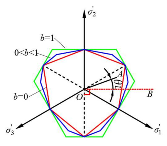
Figure 1.
Unified strength theory limit surface on deviatoric plane.
To characterize the pre-peak of stress hardening behavior of rock, we introduce hardening function h. Therefore, κ can be expressed as:
where σc is the quasi-static uniaxial compressive strength of rock.
As per [22,23], h can be defined as:
where β0 is the initial yield threshold for plastic hardening; βm is the maximum yield threshold for plastic hardening; b1 is the parameter describing the rate of hardening; and γp is the generalized plastic shear strain. As illustrated in Figure 2, rock generally does not show hardening behavior in tension. Therefore, the above hardening function is modified as:
where p is hydrostatic pressure.
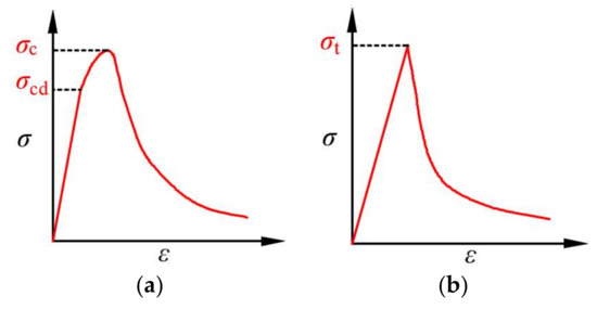
Figure 2.
Diagrammatic sketch of uniaxial stress-strain curve from rock-like materials. (a) Compression (b) tension.
2.2. Strain Rate Effect
In the practical engineering such as impact and blasting, the mechanical behaviors of the rock including deformation, damage and failure are closely related to loading rate. However, the dynamic characteristics of the rock are significantly different from the quasi-static characteristics of the rock. Therefore, the relations described in Section 2.1 need to take the strain rate effect into account. To date, a large number of studies have shown that the mechanical behaviors of rock are significantly affected by the strain rate [24] especially the strength of rock, which increases with the increase of strain rate. Based on the fracture process of the material, Grady et al. [25] divided the change process of dynamic strength of brittle materials with respect to strain rate into three stages: as shown in Figure 3, in the first stage, the quasi-static fracture process of materials does not take the inertial effect into account, and the material strength does not have an apparent rate effect, i.e., the change in material strength is not apparent with the change in strain rate. The second stage is the dynamic fracture process of the material under high strain rate, and the inertia of the material in this process cannot be ignored. The third stage occurs at ultra-high strain-rates, where thermos- and fluid-dynamical processes dominate and which no longer belongs to the category of solid mechanics, and the strain rate effect reaches the upper limit. In rock dynamics, dynamic increase factor (DIF) is usually used to reflect the influence of strain rate on the strength of rock, which is defined as the ratio of dynamic strength to quasi-static strength. The DIF can be presented as a function of the strain rate in many forms [24,26].
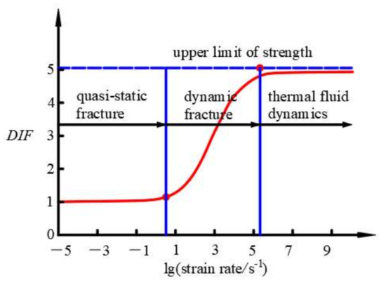
Figure 3.
Diagrammatic sketch of relationship between DIF and strain rate.
Thus, so as to obtain the accurate and reliable results, the strain rate effect should be accounted for in the numerical simulation. Based on experimental data (Figure 4), a possible relationship between DIF and strain rate can be expressed as [26,27]:
where A and B are the strain rate parameter; is the effective strain rate; is the reference strain rate, which is used to make DIF dimensionless; is the strain rate tensor.
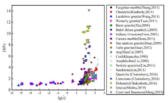
Figure 4.
Relationship between DIF and strain rate of different rock under dynamic compression conditions (data from [28,29,30,31,32,33,34,35,36,37,38,39,40,41,42,43,44]).
2.3. Plastic Flow
According to the plastic potential theory, the plastic flow rule controls the increment of plastic strain and the direction of plastic flow. The plastic flow rule can be presented as:
The plastic potential function of the unified yield criterion can be showed as [45]:
where ψ is the dilation angle. The initiation of plastic flow depends on the plastic loading conditions:
and from the plasticity consistency condition we can obtain:
The generalized plastic shear strain increment can be calculated as:
where dep is the deviatoric plastic strain increment. The deviatoric plastic strain increment can be calculated as:
where δij is the Kronecker delta; d is the volume plastic strain. Combining Equations (10), (15) and (16), we can obtain:
The relationship considering coupled elastoplasticity and damage between dσ and dε can be expressed as follows:
and substituting Equations (19) and (17) into (14), we obtain:
Finally, by combining Equations (19), (10) and (20), we can obtain the constitutive model as follows:
2.4. Damage Evolution
A large number of experimental and numerical results show that there are two damage modes of rock under complex stress: compressive shear and tensile, and their damage evolution law differs significantly [46,47,48,49]. Therefore, there are two different damage variables to capture the evolution law in this paper.
In compression, rock damage is caused not only by accumulated shear plastic strain but also by accumulated volume plastic strain due to progressive air voids collapse [14,50]. Moreover, the confining pressure has a negative effect on damage, which means that the confinement suppresses the increase of damage [51]. To characterize the above damage evolution in compression, the following damage variable from the HJC model is introduced:
where ωc is the damage variable in compression; is the plastic strain at fracture and can be calculated as:
where D1 and D2 are two contants; P* is the normalized pressure equal to P/σc; T* is the normalized tensile strength equal to σt/σc; P is the actual hydrostatic pressure; σt and σc are the unconfined uniaxial tensile strength and compressive strength, respectively.
In tension, the tensile damage of rock is related to the generalized plastic shear strain, and the tensile damage variable of rock is expressed as [3]:
where ωt is the damage variable in tension; α represents rock tensile damage parameter.
2.5. Equation of State
As presented in Figure 5, P can be divided into three zones, namely the linear elastic zone, the transition zone, and the completely dense zone.
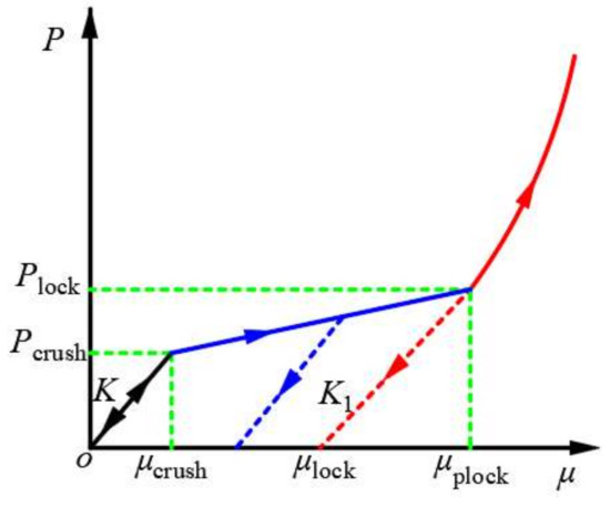
Figure 5.
Relationship between P and μ.
- (1)
- The linear elastic zone
In this zone, 0≤ μ ≤ μcrush (0 ≤ P ≤ Pcrush), the material is in an elastic state. P can be expressed as:
where μ is the volumetric strain; K is the bulk modulus; Pcrush and μcrush are the pressure and volumetric strain that occur at crushing in the uniaxial compression test, respectively.
- (2)
- The transition zone
In this region, μcrush ≤ μ ≤ μplock (Pcrush ≤ P ≤ Plock), the material is in the plastic transition stage, the internal void of the material is gradually compressed, and the plastic volume strain begins to form. P can be presented as:
where Plock is the fully dense pressure; μplock is the volumetric strain at Plock; μlock is the locking volumetric strain; K1 is the material constant.
- (3)
- The completely dense zone
In this phase, μ ≥ μplock (P ≥ Plock), the voids in the material is completely removed and the material is completely crushed. P can be presented as:
where K2 and K3 are the material constants; is the modified volumetric strain.
In the HJC model, μ = ρ/ρ0−1, μlock = ρgrain/ρ0−1, which ρ for the current density of material, ρ0 for the initial density of material, ρgrain for the grain density, but in continuum mechanics, volume strain should be presented as:
where V0 is the initial volume; V is the current volume. Therefore, the volume strain is modified in this paper to be μ = 1−ρ0/ρ. Similarly, μlock is modified as μlock = 1−ρ0/ρgrain from μlock = ρgrain/ρ0−1 and is modified as from .
3. Numerical Implementation of Constitutive Model
To facilitate the application of the model, the model is numerically implemented into the commercial finite element software LS-DYNA through Umat in this section. The numerical implementation algorithm is summarized as follows:
(1) Elastic prediction: Calculated trial stress , namely
where the subscript n denotes the previous time step, and the subscript n + 1 denotes the current time step.
(2) Substitute trial stress into Equation (1) and determine whether F (, , ωn) > 0, if F (, , ωn) ≤ 0, the material is in elastic state; if F (, , ωn) > 0, the material has entered the plastic state, and the stress should therefore be drawn back to the yield surface. In this paper, the semi-implicit stress return algorithm is adopted to make the stress return to the yield surface, as presented in Figure 6. According to the plastic mechanics, there is
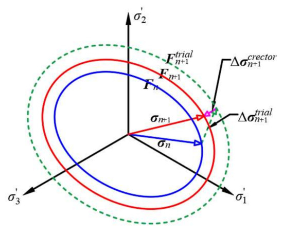
Figure 6.
Schematic diagram of stress return mapping algorithm.
The Equation (32) at the trial stress can be approximated with a first-order Taylor expansion as:
The above Δσcrector can be calculated from Equation (19) as:
Substituting Equations (10), (17) and (34) into (33), we can obtain:
(3) Calculate Δωn+1, Δ, Δσcrector.
(4) Update the variable σn+1, and ωn+1.
where Cn+1 = (Dn+1)−1.
4. Determination of Model Parameters
The determination of model parameters plays a crucial role in the development of constitutive models. The determination of model parameters is based on one or a series of standard experiments, such as the uniaxial compression test and triaxial compression test. According to the constitutive model established above, the model parameters can be divided into four categories, namely basic physical and mechanical property parameters, strength parameters, hardening parameters, and damage parameters. Basic parameters are: ρ0, E, ν, c, φ and ψ can be determined by physical test or conventional rock mechanics test. Strength parameters consist of b is from 0.5 to 1.0 suggested by Yu et al. [45]; A and B can be obtained by fitting the data from split Hopkinson pressure bar (SHPB) test. Plastic hardening parameters consist of: β0 = σcd/σc, σcd is the initial yield stress of rock [52]; βm and b1 can be fitted through the relationship between the hardening function h and the generalized shear plastic strain, γp.
Damage parameters consist of D1 and D2 are 0.04 and 1.0, respectively, as suggested by the HJC model [5]; Pcrush = σcd/3, μcrush = Pcrush/K, μlock = 1−ρ0/ρgrain [5]; K1, K2 and K3 can be determined by fitting the data from the Hugoniot experiment. Plock can be determined by the intersection point between the curve line and the straight line; α controls the softening behavior of rock, and can be calibrated with the experimental results of uniaxial tension test [53].
5. Validation of Model
To verify the accuracy of the developed constitutive model, the following four numerical examples are used: the rock uniaxial compression test (quasi-static compression), rock triaxial compression test (quasi-static compression), rock uniaxial tensile test (quasi-static tension), and rock SHPB test (dynamic).
5.1. Example 1: Rock Uniaxial Compression Test
The experimental data for this example comes from the studies on Indiana limestone by Frew et al. [27,54], Larson and Anderson [55] and Liao et al. [56]. Indiana limestone is a carbonate composed of more than 90% calcite and less than 10% quartz with a porosity of 15% and particle sizes from 0.10 mm to 0.15 mm. The parameters of this limestone are as listed in Table 1. Since this example is a quasi-static loading test, the strain rate effect is not considered, and the parameters of dynamic growth factors A and B are set to 0. The relationship between the axial stress σ1 and the confining pressure σ3 of Indiana limestone is shown in Figure 7, from which the cohesion and internal friction angle can be obtained. The relationship between h and γp of Indian limestone is showed in Figure 8, from which βm and b1 can be determined; The relationship between P and μ of Indian limestone is plotted in Figure 9, from which K1, K2, K3 and Plock can be determined. A cylindrical test sample was simulated, with the diameter of the bottom surface Ds = 50 mm and the length Ls = 100 mm, see Figure 10.

Table 1.
The parameters of limestone.
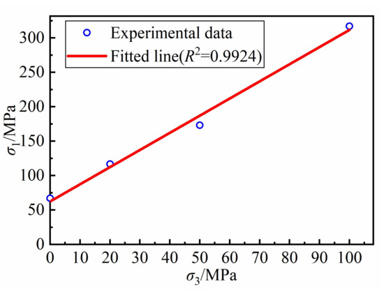
Figure 7.
Relationship between σ1 and σ3 of Indiana limestone.
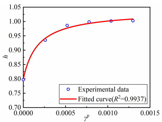
Figure 8.
Relationship between h and γp of Indian limestone.

Figure 9.
Relationship between P and μ of Indian limestone.
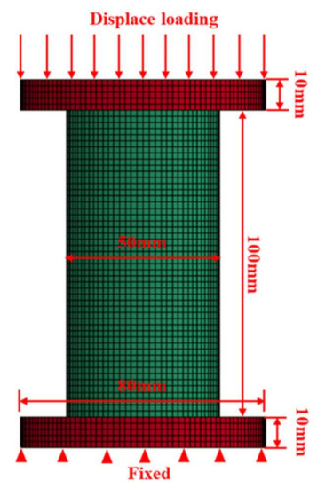
Figure 10.
Finite model and boundary condition of uniaxial compression simulation.
Figure 11 shows uniaxial compression stress-strain curve of Indian limestone. The numerical simulation undergoes three stages: linear increase, pre-peak hardening, and post-peak softening, which indicates that the numerical result is in a good agreement with the experimental data. Figure 12 shows the uniaxial compression shear damage zone of Indian limestone. It can be seen that shear failure of sample occurs under uniaxial compression. Additionally, the angle between the shear damage zone and the horizontal direction is about 57°, which agrees well with the theoretical value 57.5° calculated with θ = π/4 + φ/2 [57].
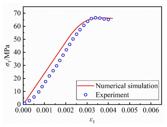
Figure 11.
Uniaxial compression stress-strain curve of Indian limestone.
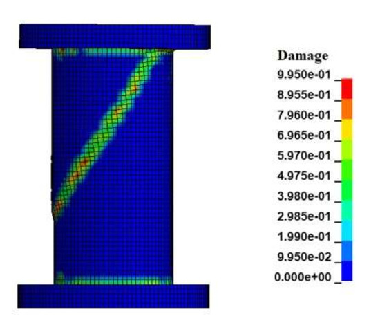
Figure 12.
Uniaxial compression shear damage zone of Indian limestone.
5.2. Example 2: Rock Triaxial Compression Test
The experimental data for this example was retrieved from compression test data of deep-metamorphic limestone [58]. The limestone is dark gray, microscopically fine grain structure, and can be regarded as an isotropic geological material. The limestone parameters are listed in Table 2, other parameters remain the same as those in example 1. Figure 13 shows the relationship between the axial stress and the confining pressure of deep-metamorphic limestone. We can then determine the internal friction angle and cohesion from the figure. Figure 14 presents the relationship between h and γp of deep-metamorphic limestone, from which βm and b1 can be determined. The geometric model (see Figure 15) used in the simulation is the same as one in example 1.
Table 2.
The parameters of limestone of deep-metamorphic limestone.
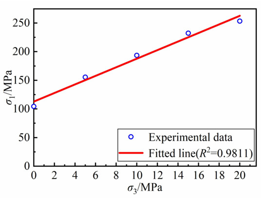
Figure 13.
Relationship between σ1 and σ3 of deep-metamorphic limestone.
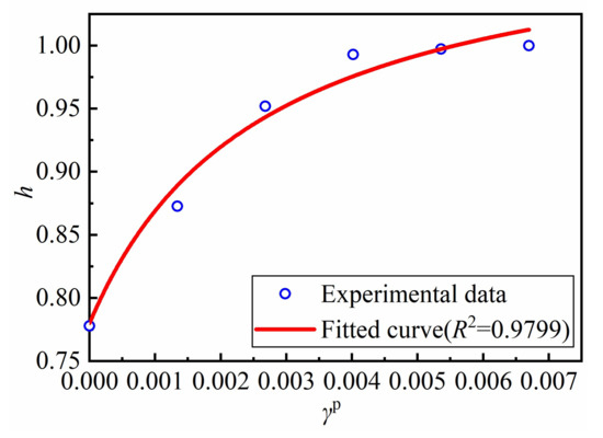
Figure 14.
Relationship between h and γp of deep-metamorphic limestone.
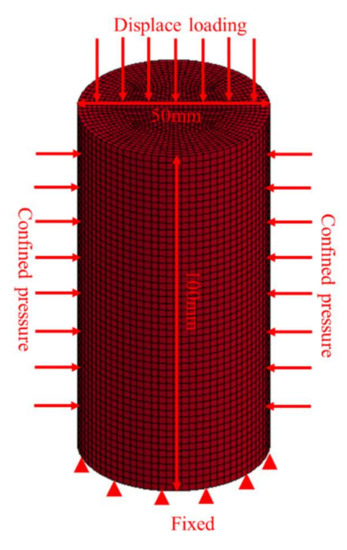
Figure 15.
Finite model and boundary condition of triaxial compression simulation.
Figure 16 presents the stress-strain relationship of deep-metamorphic limestone under different confined pressure. It can be noted that the numerical simulation agrees well with the experiment. With the increase of confining pressure, the peak stress of the curves increases and the limestone changes from brittle to ductile, which can be predicted well by the present model. It can be also observed that the model cannot predict the residual strength because there is no residual strength surface in the present model, which will be our future’s work.
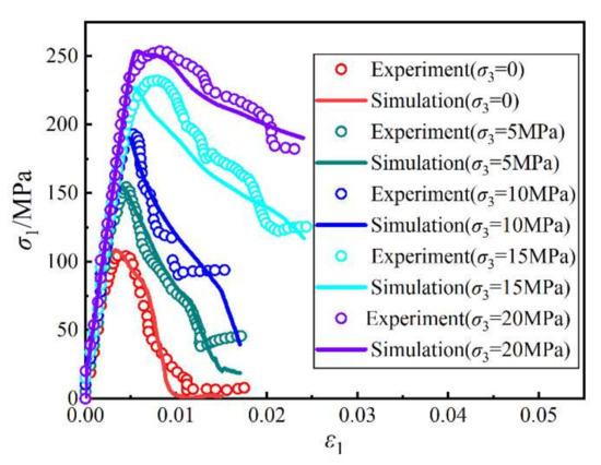
Figure 16.
Stress-strain relationship of deep-metamorphic limestone under different confined pressure.
5.3. Example 3: Rock Uniaxial Tensile Test
In this example, the tuff is subject to uniaxial tensile loading conditions and experimental data are obtained from [59]. The model parameters are showed in Table 3. Figure 17 shows the relationship between P and μ of this tuff, which is used to determine K1, K2, K3 and Plock. To keep consistent with the experimental sample, the simulated sample was also cylindrical, with the diameter of the bottom surface Ds = 25 mm and the length Ls = 50 mm, see Figure 18.
Table 3.
The parameters of tuff.
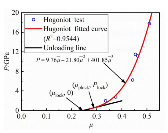
Figure 17.
Relationship between P and μ of Brisbane tuff.
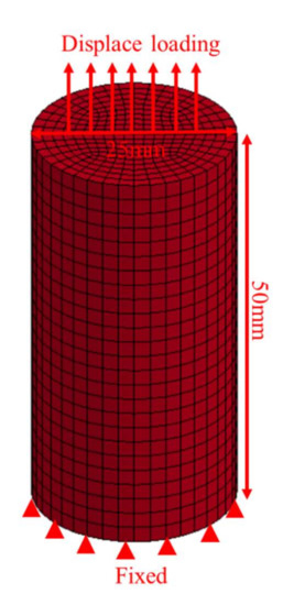
Figure 18.
Finite model and boundary condition of uniaxial tension simulation.
Figure 19 shows the uniaxial tensile stress-strain relationship of tuff. Under uniaxial tensile conditions, the stress-strain curve of tuff shows linear elastic change at first, and when the tensile stress reaches the peak, the stress drops sharply and becomes very brittle, which agrees well with the experimental results.
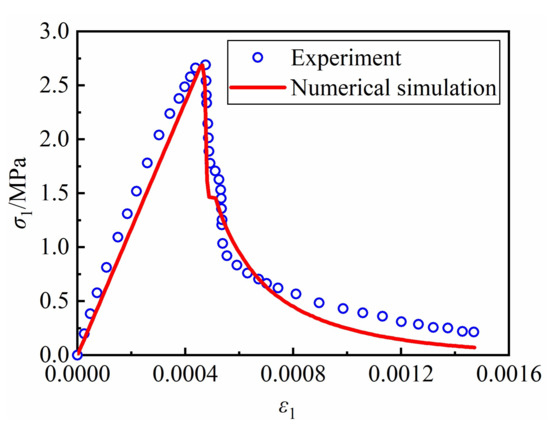
Figure 19.
Uniaxial tensile stress-strain relationship of Brisbane tuff.
5.4. Example 4: Rock SHPB Test
In this example, the Indian limestone in example 1 is taken as the object of study. Therefore, the quasi-static mechanical parameters of Indian limestone remain unchanged, and the strain rate parameters A and B are obtained by fitting the experimental data as shown Figure 20 (A = 0.3721, B = 0.1563). The geometric model of SHPB was established according to Frew et al. [27]. The SHPB test device is composed of three parts, namely the striker bar, incident bar, and the transmission bar. To modify the wave shape of the incident bar, a pulse shaper is placed between the striker bar and the incident bar. The SHPB test device is shown in Figure 21. The diameter of all the bars is 12.7 mm and three lengths of 152 mm, 2130 mm, 915 mm are used. A strain gauge is installed on the incident bar and the transmission bar, respectively, to measure the strain in the bar, and their positions are presented in Figure 22. The striker bar, incident bar, and transmission bar are made of VM350 steel and the pulse shaper is made of C11000 copper. The pulse shaper is a disk shape, with a diameter of 3.97 mm and a thickness of 0.79 mm. The parameters of VM350 steel and C11000 copper are listed in Table 4.
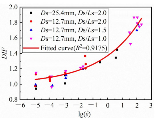
Figure 20.
Relationship between DIF and strain rate of Indian limestone.
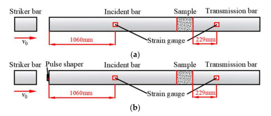
Figure 21.
Diagrammatic sketch of SHPB test device. (a) Conventional SHPB (b) Modified SHPB.
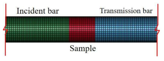
Figure 22.
Finite element model in the SHPB test.
Table 4.
The parameters of VM350 steel and C11000 copper.
The finite element model in the numerical test is shown in Figure 18. Solid 3D164 element type is adopted in the simulation. To eliminate the influence of friction in the numerical simulation, the static and dynamic friction coefficients between bar and bar and between bar and specimen are set as 0.
Figure 23 shows stress-strain curves of Indian limestone under different strain rate loading. The stress-strain curve of numerical simulation shows a linear increase at first, then plastic hardening, and then a softening behavior after the peak, which is in good agreement with the experimental results. With the increase of strain rate, the peak stress also increases, indicating that the model can capture the dynamic mechanical behavior of rocks under different strain rate loading. Figure 24 shows strain time history curve of Indian limestone obtained using a conventional SHPB test device. The agreement of the results of numerical simulation and experimental results is quite high.
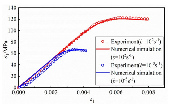
Figure 23.
Quasi-static and dynamic stress-strain curves of Indian limestone.
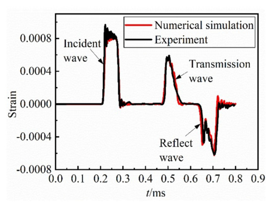
Figure 24.
Strain time history curve of Indian limestone obtained using conventional SHPB (initial velocity of striker bar is 8.05 m/s).
6. Conclusions
A dynamic coupled elastoplastic damage model for rock-like materials is presented based on UST. The model differentiates the evolution of damage in tension and compression to show the difference in mechanical behavior of rock under tension and compression. The compressive damage variable is related to the generalized shear plastic strain and volumetric plastic strain and the confining pressure. The tensile damage variable is related to the generalized shear plastic strain. The model introduces a function of strain rate to characterize the strain rate effect of rock-like materials under dynamic loading. By adopting a piecewise function, the model accounts for hardening behavior in compression and the absence of hardening behavior in tension. The volume strain from HJC model is modified to be consistent with one of continuum mechanics and correct its physical meaning. Additionally, the determination of model parameters is given in detail. Using the semi-implicit stress return mapping algorithm, the model is implemented into the finite element software LS-DYNA. The model is validated with four classic examples, including the uniaxial compression test, triaxial compression test, uniaxial tensile test, and SHPB test and the results show that the model can accurately simulate the complicated mechanical behaviors of rock-like materials under static and dynamic loading. On the other hand, the residual strength should be taken into account in the present model in the future’s work.
Author Contributions
Conceptualization, X.H., M.Z. and M.T.; methodology, X.H., M.Z. and Z.Y.; software, X.H.; validation, X.H. and M.Z.; formal analysis, M.T. and X.Z.; investigation, X.H.; resources, X.H., W.X., M.Z. and X.Z.; data curation, Z.Y.; writing—original draft preparation, X.H.; writing—review and editing, X.H. and M.Z.; visualization, X.H.; supervision, M.T. and W.X.; funding acquisition, X.H., M.Z., M.T. and X.Z. All authors have read and agreed to the published version of the manuscript.
Funding
This research was funded by the Research Fund of The State Key Laboratory of Coal Resources and safe Mining, CUMT (SKLCRSM21KF007), the National Natural Science Foundation of China (52104114 and 52074007), Collaborative innovation project of Universities in Anhui Province (GXXT-2020-056), Guidance Science and Technology Plan Projects of Huainan (2021A247).
Institutional Review Board Statement
Not applicable.
Informed Consent Statement
Not applicable.
Data Availability Statement
The data used to support the findings of the study are available from the first author upon request.
Acknowledgments
The authors would also like to express their sincere appreciation to the reviewers for their constructive comments on the revision and improvement of the manuscript. All the support is gratefully acknowledged.
Conflicts of Interest
The authors declare no conflict of interest.
References
- Ning, Y.J.; Yang, J.; An, X.M.; Ma, G.W. Modelling rock fracturing and blast-induced rock mass failure via advanced discretisation within the discontinuous deformation analysis framework. Comput. Geotech. 2011, 38, 40–49. [Google Scholar] [CrossRef]
- Yi, C.P.; Sjöberg, J.; Johansson, D.; Petropoulos, N. A numerical study of the impact of short delays on rock fragmentation. Int. J. Rock Mech. Min. Sci. 2017, 100, 250–254. [Google Scholar] [CrossRef]
- Mukherjee, M.; Nguyen, G.D.; Mir, A.; Bui, H.H.; Shen, L.M.; El-Zein, A.; Maggi, F. Capturing pressure- and rate-dependent behaviour of rocks using a new damage-plasticity model. Int. J. Impact. Eng. 2017, 110, 208–218. [Google Scholar] [CrossRef]
- Xie, L.X.; Yang, S.Q.; Gu, J.C.; Zhang, Q.B.; Lu, W.B.; Jing, H.W.; Wang, Z.L. JHR constitutive model for rock under dynamic loads. Comput. Geotech. 2019, 108, 161–172. [Google Scholar] [CrossRef]
- Holmquist, T.J.; Johnson, G.R.; Cook, W.H. A computational constitutive model for concrete subjected to large strains, high strain rates and high pressures. In Proceedings of the 14th International Symposium on Ballistics, Quebec City, QC, Canada, 26–29 September 1993. [Google Scholar]
- Murray, Y.D. Users Manual for LS-DYNA Concrete Material Model 159 (No. FHWA-HRT-05-062); Federal Highway Administration, Office of Research, Development, and Technology: Washington, DC, USA, 2007.
- Malvar, L.J.; Crawford, J.E.; Wesevich, J.W.; Simons, D. A plasticity concrete material model for DYNA3D. Int. J. Impact. Eng. 1997, 19, 847–873. [Google Scholar] [CrossRef]
- Riedel, W.; Thoma, K.; Hiermaier, S.; Schmolinske, E. Penetration of Reinforced Concrete by BETA-B-500 Numerical Analysis using a New Macroscopic Concrete Model for Hydrocodes. In Proceedings of the 9th International Symposium on Interaction of the Effects of Munitions with Structures, Berlin-Strausberg, Germany, 3–7 May 1999. [Google Scholar]
- Polanco-Loria, M.; Hopperstad, O.S.; Børvik, T.; Berstad, T. Numerical predictions of ballistic limits for concrete slabs using a modified version of the HJC concrete model. Int. J. Impact. Eng. 2008, 35, 290–303. [Google Scholar] [CrossRef]
- Liu, F.; Li, Q.M. Strain-rate effect on the compressive strength of brittle materials and its implementation into material strength model. Int. J. Impact. Eng. 2019, 130, 113–123. [Google Scholar] [CrossRef]
- Jiang, H.; Zhao, J.D. Calibration of the continuous surface cap model for concrete. Finite Elem. Anal. Des. 2015, 97, 1–19. [Google Scholar] [CrossRef]
- Kong, X.Z.; Fang, Q.; Li, Q.M.; Wu, H.; Crawford, J.E. Modified K&C model for cratering and scabbing of concrete slabs under projectile impact. Int. J. Impact. Eng. 2017, 108, 217–228. [Google Scholar] [CrossRef] [Green Version]
- Tu, Z.G.; Lu, Y. Modifications of RHT material model for improved numerical simulation of dynamic response of concrete. Int. J. Impact. Eng. 2010, 37, 1072–1082. [Google Scholar] [CrossRef] [Green Version]
- Li, H.Y.; Shi, G.Y. A dynamic material model for rock materials under conditions of high confining pressures and high strain rates. Int. J. Impact. Eng. 2016, 89, 38–48. [Google Scholar] [CrossRef]
- Kong, X.Z.; Fang, Q.; Wu, H.; Peng, Y. Numerical predictions of cratering and scabbing in concrete slabs subjected to projectile impact using a modified version of HJC material model. Int. J. Impact. Eng. 2016, 95, 61–71. [Google Scholar] [CrossRef]
- Leppänen, J. Concrete subjected to projectile and fragment impacts: Modelling of crack softening and strain rate dependency in tension. Int. J. Impact. Eng. 2006, 32, 1828–1841. [Google Scholar] [CrossRef]
- Johnson, G.R.; Holmquist, T.J. An Improved Computational Constitutive Model for Brittle Materials. AIP. Conf. Proc. 1994, 309, 981–984. [Google Scholar]
- Furlong, J.; Alme, M.; Rajendran, A. Numerical modelling of ceramic penetration experiments. In Proceedings of the Fourth TACOM Armor Coordinating Conference for Light Combat Vehicles, Naval Postgraduate School, Monterey, CA, USA, 12 January 2022. [Google Scholar]
- Liu, L.; Katsabanis, P.D. Development of a continuum damage model for blasting analysis. Int. J. Rock Mech. Min. Sci. 1997, 34, 217–231. [Google Scholar] [CrossRef]
- Yu, M.H.; Zan, Y.W.; Zhao, J.; Yoshimine, M. A unified Strength criterion for rock material. Int. J. Rock Mech. Min. Sci. 2002, 39, 975–989. [Google Scholar] [CrossRef]
- Deng, L.S.; Fan, W.; Yu, M.H. Parametric study of a loess slope based on unified strength theory. Eng. Geol. 2018, 233, 98–110. [Google Scholar] [CrossRef]
- Chen, L.; Shao, J.F.; Huang, H.W. Coupled elasto-plastic damage modeling of anisotropic rocks. Comput. Geotech. 2010, 37, 187–194. [Google Scholar] [CrossRef]
- Chen, L.; Wang, C.P.; Liu, J.F.; Liu, J.; Wang, J.; Jia, F.; Shao, J. Damage and plastic deformation modeling of Beishan granite under compressive stress conditions. Rock Mech. Rock Eng. 2015, 48, 1623–1633. [Google Scholar] [CrossRef]
- Zhang, Q.B.; Zhao, J. A review of dynamic experimental techniques and mechanical behavior of rock materials. Rock Mech. Rock Eng. 2014, 47, 1411–1478. [Google Scholar] [CrossRef] [Green Version]
- Gary, G.; Bailly, P. Behaviour of quasi-brittle material at high strain rate. Experiment and modelling. Eur. J. Mech-Solid. 1998, 17, 403–420. [Google Scholar] [CrossRef] [Green Version]
- Lu, D.C.; Wang, G.S.; Du, X.L.; Wang, Y. A nonlinear dynamic uniaxial strength criterion that considers the ultimate dynamic strength of concrete. Int. J. Impact. Eng. 2017, 103, 124–137. [Google Scholar] [CrossRef]
- Grigoriev, A.S.; Shilko, E.V.; Skripnyak, V.A.; Psakhie, S.G. Kinetic approach to the development of computational dynamic models for brittle solids. Int. J. Impact. Eng. 2019, 123, 14–25. [Google Scholar] [CrossRef]
- Zhang, Q.B.; Zhao, J. Determination of mechanical properties and full-field strain measurements of rock material under dynamic loads. Int. J. Rock Mech. Min. Sci. 2013, 60, 423–439. [Google Scholar] [CrossRef]
- Kimberley, J.; Ramesh, K.T. The dynamic strength of an ordinary chondrite. Meteorit. Planet. Sci. 2011, 46, 1653–1669. [Google Scholar] [CrossRef]
- Wang, Y.N.; Tonon, F. Dynamic validation of a discrete element code in modeling rock fragmentation. Int. J. Rock Mech. Min. Sci. 2011, 48, 535–545. [Google Scholar] [CrossRef]
- Yuan, F.P.; Prakash, V.; Tullis, T. Origin of pulverized rocks during earthquake fault rupture. J. Geophys. Res-Sol. Earth 2011, 116, B06309. [Google Scholar] [CrossRef]
- Xia, K.; Nasseri, M.H.B.; Mohanty, B.; Lu, F.; Chen, R.; Luo, S.N. Effects of microstructures on dynamic compression of Barre granite. Int. J. Rock Mech. Min. Sci. 2008, 45, 879–887. [Google Scholar] [CrossRef]
- Li, X.B.; Lok, T.S.; Zhao, J. Dynamic Characteristics of Granite Subjected to Intermediate Loading Rate. Rock Mech. Rock Eng. 2005, 38, 21–39. [Google Scholar] [CrossRef]
- Doan, M.-L.; Billi, A. High strain rate damage of Carrara marble. Geophys. Res. Lett. 2011, 38, L19302. [Google Scholar] [CrossRef]
- Doan, M.-L.; D’hour, V. Effect of initial damage on rock pulverization along faults. J. Struct. Geol. 2012, 45, 113–124. [Google Scholar] [CrossRef]
- Doan, M.-L.; Gary, G. Rock pulverization at high strain rate near the San Andreas fault. Nat. Geosci. 2009, 2, 709–712. [Google Scholar] [CrossRef] [Green Version]
- Cai, M.; Kaiser, P.K.; Suorineni, F.; Su, K. A study on the dynamic behavior of the Meuse/Haute-Marne argillite. Phys. Chem. Earth 2007, 32, 907–916. [Google Scholar] [CrossRef]
- Klepaczko, J.R. Behavior of rock-like materials at high strain rates in compression. Int. J. Plast. 1990, 6, 415–432. [Google Scholar] [CrossRef]
- Liu, J.Z.; Xu, J.Y.; Lv, X.C.; Zhang, L.; Wang, Z.D. Experimental study on dynamic mechanical properties of amphibolites under impact compressive loading. Chin. J. Rock Mech. Eng. 2009, 28, 2113–2120. [Google Scholar] [CrossRef]
- Liu, S.; Xu, J.Y.; Liu, J.; Lv, X.C. SHPB experimental study of sericite-quartz schist and sandstone. Chin. J. Rock Mech. Eng. 2011, 30, 1864–1871. [Google Scholar]
- Chakraborty, T.; Mishra, S.; Loukus, J.; Halonen, B.; Brady, B. Characterization of three Himalayan rocks using a split Hopkinson pressure bar. Int. J. Rock Mech. Min. Sci. 2016, 85, 112–118. [Google Scholar] [CrossRef]
- Mishra, S.; Khetwal, A.; Chakraborty, T. Dynamic Characterisation of Gneiss. Rock Eng. Rock Mech. 2019, 52, 61–81. [Google Scholar] [CrossRef]
- Meng, Q.S.; Fan, C.; Zeng, W.X.; Yu, K.F. Tests on dynamic properties of coral-reef limestone in South China Sea. Rock Soil. Mech. 2019, 40, 183–190. [Google Scholar] [CrossRef]
- Frew, D.J.; Forrestal, M.J.; Chen, W. A Split Hopkinson Pressure Bar Technique to Determine Compressive Stress-strain Data for Rock Materials. Exp. Mech. 2001, 46, 40–46. [Google Scholar] [CrossRef]
- Yu, M.H.; Yang, S.Y.; Fan, S.C.; Ma, G.W. Unified elasto-plastic associated and non-associated constitutive model and its engineering applications. Comput. Struct. 1999, 71, 627–636. [Google Scholar] [CrossRef]
- Kaiser, P.K.; Diederichs, M.S.; Eberhardt, E. Damage initiation and propagation in hard rock during tunnelling and the influence of near-face stress rotation. Int. J. Rock Mech. Min. Sci. 2004, 41, 785–812. [Google Scholar] [CrossRef]
- Zhu, Z.M.; Mohanty, B.; Xie, H.P. Numerical investigation of blasting-induced crack initiation and propagation in rocks. Int. J. Rock Mech. Min. Sci. 2007, 44, 412–424. [Google Scholar] [CrossRef]
- Ma, G.W.; An, X.M. Numerical simulation of blasting-induced rock fractures. Int. J. Rock Mech. Min. Sci. 2008, 45, 966–975. [Google Scholar] [CrossRef]
- Yao, C.; Shao, J.F.; Jiang, Q.H.; Zhou, C.B. Numerical study of excavation induced fractures using an extended rigid block spring method. Comput. Geotech. 2017, 85, 368–383. [Google Scholar] [CrossRef]
- Yang, L.; Lin, X.S.; Li, H.Y.; Gravina, R.J. A new constitutive model for steel fiber reinforced concrete subjected to dynamic loads. Compos. Struct. 2019, 221, 110849. [Google Scholar] [CrossRef]
- Zhang, H.M.; Lei, L.N.; Yang, G.S. Characteristic and representative model of rock under constant confining stress. J. China Univ. Mining. Technol. 2015, 44, 59–63. [Google Scholar]
- Zhang, J.C.; Xu, W.Y.; Wang, H.L.; Wang, R.B.; Meng, Q.X.; Du, S.W. A coupled elastoplastic damage model for brittle rocks and its application in modelling underground excavation. Int. J. Rock Mech. Min. Sci. 2016, 84, 130–141. [Google Scholar] [CrossRef]
- Le, L.A.; Nguyen, G.D.; Bui, H.H.; Sheikh, A.H.; Kotousov, A.; Khanna, A. Modelling jointed rock mass as a continuum with an embedded cohesive-frictional model. Eng. Geol. 2017, 228, 107–120. [Google Scholar] [CrossRef]
- Frew, D.J. Dynamic Response of Brittle Materials from Penetration and Split Hopkison Pressure Bar Experiments; Arizona State University: Phoenix, AZ, USA, 2000. [Google Scholar]
- Larson, D.B.; Anderson, G.D. Plane shock wave studies of porous geologic media. J. Geophys. Res. Solid Earth 1979, 84, 4592–4600. [Google Scholar] [CrossRef]
- Liao, Z.Y.; Zhu, J.B.; Xia, K.W. Determination of Dynamic Compressive and Tensile Behavior of Rocks from Numerical Tests of Split Hopkinson Pressure and Tension Bars. Rock Mech. Rock Eng. 2016, 49, 3917–3934. [Google Scholar] [CrossRef]
- Arthur, J.R.F.; Dunstan, T.; Al-ani, Q.A.J.L.; Assadi, A. Plastic deformation and failure in granular media. Geotechnique 1977, 27, 53–74. [Google Scholar] [CrossRef]
- Zhang, J.C. Experimental and Modelling Investigations of the Coupled Elastoplastic Damage of a Quasi-brittle Rock. Rock Mech. Rock Eng. 2018, 51, 465–478. [Google Scholar] [CrossRef]
- Okubo, S.; Fukui, K. Complete stress-strain curves for various rock types in uniaxial tension. Int. J. Rock Mech. Min. Sci. 1996, 33, 549–556. [Google Scholar] [CrossRef]
Publisher’s Note: MDPI stays neutral with regard to jurisdictional claims in published maps and institutional affiliations. |
© 2022 by the authors. Licensee MDPI, Basel, Switzerland. This article is an open access article distributed under the terms and conditions of the Creative Commons Attribution (CC BY) license (https://creativecommons.org/licenses/by/4.0/).