Simulation of the Frequency Response Analysis of Gas Diffusion in Zeolites by Means of Computational Fluid Dynamics

Abstract

Frequency response (FR) analysis allows the characterization of gas diffusion occurring within a porous solid system. The shape of the pressure response curves obtained after a volume modulation in the reactor gives essential information about the gas adsorption and desorption properties of the porous material, e.g., zeolites, which is in contact with a certain gas environment, as well as information about the transport phenomena such as diffusion. In this work, a simulation model developed in COMSOL Multiphysics^® is introduced to reproduce the experimental behavior of the tested solid/gas systems. This approach covers, for the first time, a coupling of computational fluid dynamics (CFD), porous media flow, and a customized mass adsorption/desorption function to simulate the behavior of real frequency response systems. The simulation results are compared to experimental data obtained from the interaction of propane in MFI zeolites as well as additional data from the literature to evaluate the model validity. Furthermore, a small variation study of the effect of simulation parameters such as the mass of the sample, bed porosity, or geometry is performed and analyzed. The essential advantage of this model with respect to other analytical approaches is to observe the spatial pressure and adsorption distribution (along with other local effects) of the gas within the porous material. Thus, local environments can be visualized, and non-idealities can, therefore, be detected in contrast to the general integral simulation approach.

1. Introduction

The characterization of the gas diffusion properties of porous materials, such as zeolites, holds significant relevance across a broad spectrum of applications: from characterizing gas-specific adsorbents to catalyst design [1,2]. Various time-resolved characterization methods are available, including the temporal analysis of products (TAP) [3,4,5], electrochemical impedance spectroscopy (EIS) [6,7], or frequency response (FR) [2,8].

In this work, our focus is on FR analysis among the different characterization options. The FR method is advantageous for investigating mass transfer phenomena and determining kinetic parameters for gases within porous materials [9,10]. FR is a macroscopic measurement technique well-suited for operating under both non-equilibrium and nearly equilibrium conditions. In the case of the volume-swing frequency response (VSFR) [11,12,13], a very small periodic volume perturbation to ensure linearity is introduced in a closed system containing the sample material and gas in sorption equilibrium. This perturbation activates the different mass transport processes causing a pressure response. The amplitude and phase shift of the pressure response depend on the relaxation times of mass transfer processes, such as adsorption or desorption. As a result, this method allows for characterizing the intricate processes within the pore structure, enabling the distinction between dynamic characteristics, like effective diffusivity or adsorption kinetics, and capacity-related attributes, including pore volume or modifications in surface loading.

The function of volume modulation can vary depending on the construction of the FR device. The most common approach is based on a sinusoidal waveform [8,10,11]. The pressure response in such systems also exhibits a waveform function with varying amplitude and phase. The information provided by these observations yields what is known as frequency-dependent "characteristic FR functions" [14,15]. These functions depend on the measured relative pressure amplitude (with and without sample material) and the phase shift between them. A qualitative example is shown in Figure 1. In the figure, coupled mass transfer processes, such as adsorption and diffusion, operating on different scales can be observed. In the qualitative example, the time constants of two processes are discernible at the peak points on the characteristic curves, with slower processes manifesting at low frequencies and faster processes at higher frequencies. With FR, even the effect of surface or film resistances can be obtained in the form of a diffusion coefficient [16,17].

Other variations of VSFR-based devices include single-step FR (SSFR) and square wave-based volume modulation [14,18,19]. In the first case, only one oscillation of the square function is applied as a perturbation to the system. These experiments are particularly useful for describing and determining intracrystalline diffusion coefficients of alkanes in microporous solids through the analysis of the pressure curve decay [14,20,21]. In the second case, when a square wave function serves as the perturbation input, both approaches can be partially investigated. On one hand, FR parameters (amplitude and phase lag) can be derived from the corresponding sinusoidal equivalent function, obtained through Fourier transformations (frequency decomposition) of the input and output functions [22,23]. In other words, a single measurement at one frequency can already unveil a significant part of the FR characteristic curves for specific mass transfer processes. On the other hand, the decay of the pressure response, as in the case of SSFR, can also be observed and analyzed at different frequencies (see the decay of the pressure curve at every cycle in Figure 2b). This increases the amount of information registered in every measurement.

One of the challenges of the square wave volume modulation method is how to correctly interpret the obtained information. Most analytical approaches aim to determine an equivalent diffusion coefficient for the transport phenomena occurring in the device. However, without prior information, it becomes a complex task to distinguish which specific phenomenon is being measured or whether other unexpected phenomena are influencing the results. For this reason, a simulation model that allows for the direct simulation of the physics can be instrumental in investigating the specific mass transport processes taking place in the system.

The Chair of Thermodynamics at the Technische Universität Dresden possesses a custom FR device for studying diffusion phenomena. Its technical characteristics are described in the work of Grün et al. [24]. The studied characterization process consists in the volume-swing frequency response (VSFR). In the volume modulation unit, the device is loaded with the porous material and the chosen gas at a certain pressure. The volume is modulated by a moving metal plate driven by two electromagnetic coils, resulting in a square waveform for the volume variation (see Figure 2a). This input generates a pressure response that is registered by a differential pressure sensor (see Figure 2b). As mentioned earlier, the amplitude, phase shift, and decay of the pressure curve provide crucial information about the diffusion processes occurring within the selected gas-porous material system, which, in this work, is focused on zeolite systems.

In this context, numerical simulations about the experimental procedure can serve both as (i) a further evaluation tool to investigate the phenomena involved during the FR process as well as (ii) an instrument to obtain a visualization of the local adsorption effects within the fixed bed of porous sample. Furthermore, it can save experimental time by reducing the number of measurements needed for characterizing the porous material under the influence of a specific adsorbing gas.

In this work, such a simulation model based on computational fluid dynamics (CFD) is, to the best of our knowledge, for the first time fully described (a preview was shown in [24]). The model, built in COMSOL Multiphysics^® 6.0 (COMSOL, Inc., Kingston, Australia), is compared to performed measurements as well as to similar experimental values from the literature.

2. Materials and Methods

In Section 2.1, the model-governing equations, boundary conditions, and the coupling of various involved physics will be introduced. In Section 2.2, details about the evaluated gas/solid systems and the corresponding properties will be provided. In Section 2.3, additional simulation details, including the mesh used and solvers will be described.

2.1. Model Definition

The model employs four distinct physics (see Figure 3) applied on a 2D-axilsymmetric geometry. The simulated geometry consists exclusively of the volume modulation unit, encompassing the sample chamber (depicted in red in Figure 3), the moving plate (located on the top surface in Figure 3), and the connecting pipe between these components. The dimensions of the geometry are provided in Figure 4. The model incorporates four simulated physics components:

• The arbitrary Lagrangian–Eulerian (ALE) method, in the form of a deformed geometry that simulates the movement of the metal plate, which effectively produces the volume modulation.
• The computational fluid dynamics (CFD) module that uses the Navier–Stokes equations for the transport of the fluid in the region where no porous material is present.
• The porous media flow that describes the transport of the fluid within the porous material.
• Additionally, an equation describing gas adsorption/desorption and its impact of pressure and transport properties is included within the porous media flow formulation.

These effects and boundary conditions are explained in the following subsections, in that order.

2.1.1. Arbitrary Lagrangian–Eulerian (ALE) Method

The first simulation physics are given by the movement of the plate. COMSOL Multiphysics^® offers two specific options for these simulations: moving mesh and deformed geometry, both based on the ALE method [25,26,27]. To understand the modeling process, it is necessary to explain how COMSOL Multiphysics^® handles different reference systems when using the ALE formulation.

When creating a model in COMSOL Multiphysics^®, it generates four different coordinate systems or frames [28] (in cylindrical coordinates):

• Spatial frame: this is the standard frame based on the Eulerian or Euclidean formulation. It remains fixed and provides a reference point for observing any movement or deformation in the generated geometry. The coordinates are described as r, phi, z.
• Material frame: this reference system follows the Lagrangian formulation. It is a local coordinate system that remains consistent even if the system undergoes deformation. For a deformed solid, the local coordinates of the material frame, R, PHI, Z, would adapt to the deformation. However, from the point of view of the spatial frame, R, PHI, Z, it would appear curvilinear.
• Geometry frame: this reference system is created from the initial geometry of the system before any movement or deformation occurs. It does not change during the simulations. The coordinates are R_g, PHI_g, Z_g.
• Mesh frame: this is the reference system used in computational finite element method (FEM) calculations after the geometry frame has been meshed. It is recalculated whenever there is a remeshing step or a mesh deformation. The coordinates R_m, PHI_m, Z_m are used to locate the different node points of the meshed structure.

The mapping functions between all these coordinate systems are automatically handled by the software. Initially, after creating the geometry frame, the mapping to the mesh frame (mesh elements and nodes) is generated. The information in the mesh frame is used by the solvers in COMSOL Multiphysics^® for model computation. The geometry frame is also mapped onto the material frame, which, in turn, is mapped onto the spatial frame. If the ALE formulation is not employed, a unit map function is defined between the geometry, material, and spatial frames and they coincide. However, when the ALE formulation is needed due to geometrical movement or deformation, the mapping functions, including the one of the mesh frame, are correspondingly modified.

In COMSOL Multiphysics^®, when enabling the ALE formulation, two different cases can occur. The first case is the “moving mesh” physics in the software. In this formulation, the movement/deformation is defined in the mapping function between the material frame (Lagrangian) and spatial frame (Eulerian). This is typical for Fluid–Structure Interaction (FSI) models [29,30,31]. The deformation is only seen from the spatial frame where the fluid mechanics are simulated in Eulerian form, while structural mechanics of the solid are formulated in the Lagrangian form in the locally fixed material frame. This, in practice, forces the conservation of the solid material volume. However, this is not the approach used in this work.

The second case is the “deformed geometry” in the software. In this approach, the movement/deformation is defined in the mapping function between the geometry frame and the material (Lagrangian) frame. In other words, the Lagrangian and Eulerian frames coincide (r, phi, z = R, PHI, Z) and both see a morphological change compared to the initial geometry stored in the geometry frame. If the domain would describe a solid, this would be equivalent to adding or removing material from the domain [32,33]. This approach is chosen in this work because the domain physically changes in the real system without deformation, with the domain volume effectively added (expansion, upper position of the plate) or removed (compression, lower position of the plate).

In order to change the geometry shape, the boundary conditions that define the plate movement must be defined. A square wave function is used with an amplitude value corresponding to the movement of the plate. This square waveform, formally named wv1, is applied to the top geometry, where the plate is located (see Figure 2 and Figure 5). The signal’s frequency and the transition zone, which smooths the signal’s rise and fall when transitioning from top to bottom or vice versa for simulation stability, will be detailed for each comparison. This transition zone will be referred to as the peak-to-peak time t_pp henceforth (see Figure 5). To prevent derivative instabilities, the signal’s rise and fall are approximated by a second-order curve. The boundary condition at the plate (formally on the material frame as defined by the software) would be as follows:

$$\left\{\begin{array}{c}z\left(t\right)=Z\left(t\right)=wv1\left(t, f,t_{\mathrm{pp}}\right)\\ r\left(t\right)=R\left(t\right)=0\end{array}\right.$$

(1)

where f is the frequency and t corresponds to the time. Additionally, the plate cannot move horizontally.

For the lateral side of the geometry in contact with the moving plate, a zero normal displacement condition is imposed to permit the plate’s vertical movement (see Figure 5). The boundary condition is as follows:

$$r\left(t\right)=R\left(t\right)=0$$

(2)

For the rest of the geometry boundaries, a no-displacement boundary condition is enforced as follows:

$$\left\{\begin{array}{c}z\left(t\right)=Z\left(t\right)=0\\ r\left(t\right)=R\left(t\right)=0\end{array}\right.$$

(3)

After defining the boundary conditions, it is crucial to ensure smooth mesh deformation to prevent geometry collapse or inverted mesh elements. Several smoothing methods are available, each with varying complexity and computational costs. Three commonly used methods include [34,35,36,37,38]: (i) elliptic mesh generation smoothing, such as the Laplacian smoothing [35,39,40,41,42,43,44,45]; (ii) forced-based smoothing, using spring-like methods [34,46]; (iii) smoothing methods based on structural mechanics, such as elastic smoothing [36,37,47] (sometimes with the combination of the FEM Jacobian-based stiffening [48,49]) or hyperelastic smoothing [50,51,52].

The choice of the smoothing method depends on simulation needs [42]. Structural mechanics-based methods are suitable when the deformations of the solid are relevant to the physics being simulated, as in Fluid–Structure Interaction (FSI) applications. However, in this work, the structural behavior of the moving plate is not a crucial factor. The plate serves to compress and expand the fluid domain while coupling the plate velocity to the fluid velocity. Using complex structural mechanics-based methods (group iii) would significantly increase the computation time without substantially improving simulation results.

Another scenario for using complex smoothing methods is when dealing with large deformations/displacements [48,49,50,51,52]. These methods can provide more precise results without remeshing. However, like in this work, typical FR systems involve only a small volume variation, usually around 1% or lower, which is a required condition to assume linearity for further analytical analysis [10,14,15,53,54]. Additionally, the primary volume variation occurs in the radial dimension rather than in vertical displacement.

For instance, in our setup, the diameter of the plate is 46 mm, while the vertical displacement is only of ±0.5 mm. When compared to the overall height of 244.2 mm of the simulated system, the vertical displacement corresponds to approximately 0.20% of the vertical dimension. Given the small change in the vertical dimension, the limited relevance of solid stresses/deformation, and the computational cost-effectiveness, the Laplacian smoothing approach was chosen for the simulation. To validate this choice, a simulation with a compression and expansion of ±1 mm (double the expected change before volume correction) was performed. The results (Figure 6) showed no element inversion or mesh instability.

Laplacian smoothing offers two variants: solving the Laplace equation for coordinate positions or coordinate velocities [45,55,56]. For stationary problems where the physics are solved after a specified boundary displacement, smoothing the coordinate positions is sufficient to regularize the effect of displacement across the domain. However, in time-dependent problems, solving the Laplacian of coordinate velocities is preferred. This approach prevents the introduction of velocities in directions other than the boundary velocity at adjacent mesh points, while preserving initial element size ratios and reducing the risk of element inversions during time-dependent simulations [35,43,45]. Even when movements are relatively small, it is essential to check the mesh elements after each simulation run and choose an appropriate mesh element size. If the movement exceeds the mesh element size, the likelihood of element inversion increases.

The used Laplacian smoothing of the coordinate velocities [28,35,57] is expressed as follows:

$${\left.{\nabla }^2\overrightarrow{c}\right|}_{R_{\mathrm{g}},PH{I}_{\mathrm{g}},Z_{\mathrm{g}}}=0$$

(4)

where $\overrightarrow{c}$ represents the velocity in both the spatial and material frames (which are equivalent in this formulation). The Laplacian is computed with respect to the geometry frame coordinates.

It is worth noting that COMSOL Multiphysics^® automatically handles frame mapping when using ALE. In other software implementations, manual modifications may be necessary for equations solved in either the spatial or material frame. In COMSOL Multiphysics^®, the equations sent to the solver are those solved in the mesh frame (often referred to as the ALE frame in other works). When the ALE method is enabled, any time derivative must be corrected according to the frame velocity $\overrightarrow{c}$. For the time derivative of any function f in the spatial/Eulerian reference system, the solver computes it as follows [28,38,42,58,59,60,61,62]:

$${\left.\frac{\partial f}{\partial t}\right|}_{r,phi,, z}={\left.\frac{\partial f}{\partial t}\right|}_{R_{\mathrm{m}},PH{I}_{\mathrm{m}},Z_{\mathrm{m}}}-\overrightarrow{c}{\left. \overrightarrow{\nabla }f\right|}_{r,phi, z}$$

(5)

where ${\left. \overrightarrow{\nabla }f\right|}_{r,phi, z}$ is the gradient of the function f with respect to the spatial frame.

After the ALE formulation is complete, the movement of the plate must be transferred to the fluid, which is the next step of the model.

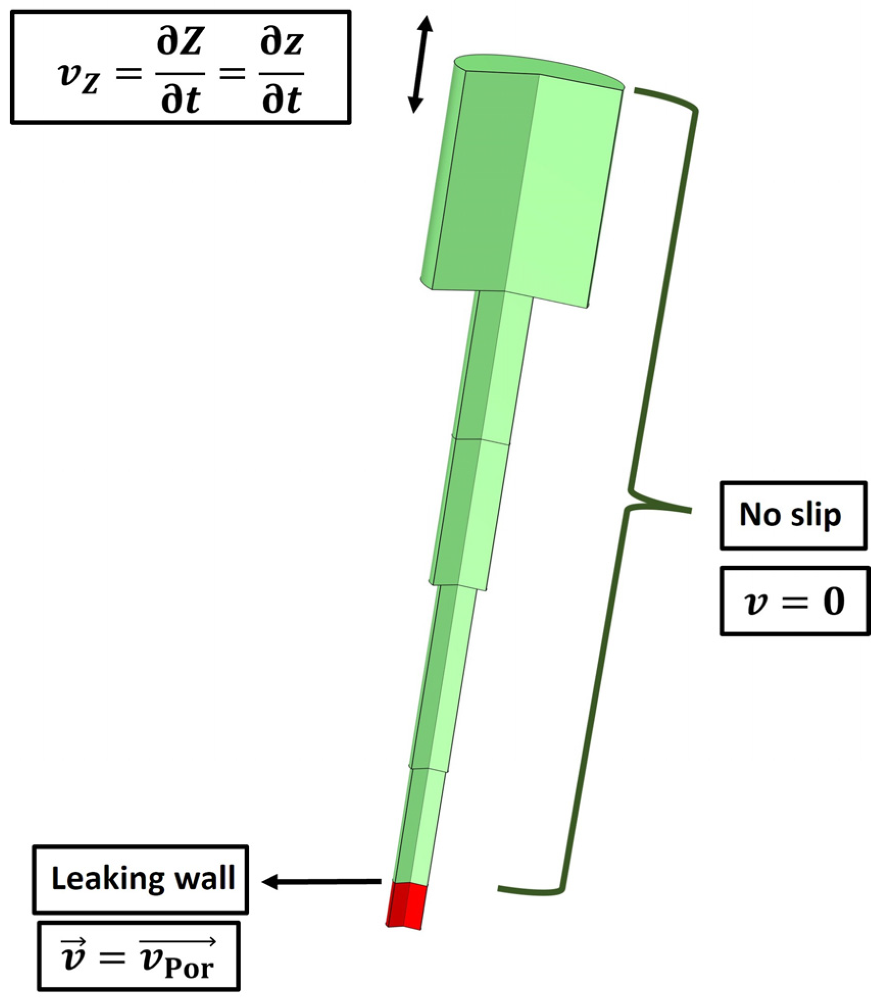
2.1.2. Computational Fluid Dynamics (CFD) Simulation for Fluid Transport

In the simulation domain where no porous material is present, CFD is used to solve the transport physics of the fluid. The governing equation is the known compressible Navier–Stokes equation [63] in the spatial frame:

$$\left\{\begin{array}{c}\frac{\partial \rho }{\partial t}+\overrightarrow{\nabla }\left(\rho \overrightarrow{v}\right)=0\\ \rho \frac{\partial \overrightarrow{v}}{\partial t}+\rho \left(\overrightarrow{v}\overrightarrow{\nabla }\right)\overrightarrow{v}=-\overrightarrow{\nabla }p+\overrightarrow{\nabla }\left(\mu \left(\nabla \overrightarrow{v}+{\left(\nabla \overrightarrow{v}\right)}^{\mathrm{T}}\right)-\frac{2}{3}\mu \left(\nabla \overrightarrow{v}\right)I\right)\end{array}\right.$$

(6)

where ρ is the density, v is the fluid velocity, p is the pressure, μ is the viscosity, T is transposed tensor, and I is the identity tensor. This formulation neglects the buoyancy effects as the system is assumed to be isothermal. In order to reduce the computational cost, a further simplification can be performed. As a Reynolds number (Re) much lower than one is expected (verified during the simulations), the Stokes flow approach can be employed [64,65]. The Stokes flow neglects the inertial terms of the Navier–Stokes equation. The local Reynolds number is defined as follows:

$$Re=\frac{\rho \left|\overrightarrow{v}\right|h}{\mu }\ll 1$$

(7)

where h is the size of the simulation mesh element. With this assumption, the Navier–Stokes equation is reduced to the following:

$$\left\{\begin{array}{c}\frac{\partial \rho }{\partial t}+\overrightarrow{\nabla }\left(\rho \overrightarrow{v}\right)=0\\ \rho \frac{\partial \overrightarrow{v}}{\partial t}=-\overrightarrow{\nabla }p+\overrightarrow{\nabla }\left(\mu \left(\nabla \overrightarrow{v}+{\left(\nabla \overrightarrow{v}\right)}^{\mathrm{T}}\right)-\frac{2}{3}\mu \left(\nabla \overrightarrow{v}\right)I\right)\end{array}\right.$$

(8)

For other software, or internally for COMSOL Multiphysics^®, the equations must be corrected with the expression of Equation (5) in the mesh frame, due to the ALE formulation:

$$\left\{\begin{array}{c}\frac{\partial \rho }{\partial t}+\overrightarrow{\nabla }\left(\rho \overrightarrow{v}\right)-\overrightarrow{\nabla }\left(\rho \overrightarrow{c}\right)=0\\ \rho \frac{\partial \overrightarrow{v}}{\partial t}-\rho \left(\overrightarrow{c} \overrightarrow{\nabla }\right)\overrightarrow{v}=-\overrightarrow{\nabla }p+\overrightarrow{\nabla }\left(\mu \left(\nabla \overrightarrow{v}+{\left(\nabla \overrightarrow{v}\right)}^{\mathrm{T}}\right)-\frac{2}{3}\mu \left(\nabla \overrightarrow{v}\right)I\right)\end{array}\right.$$

(9)

where the frame notations of the derivatives are dropped as from the computational point of view, there is no difference. Equation (9) is the so-called ALE Navier–Stokes equation in other works [38,60,61,62] but without the inertial effects.

The boundary conditions are the following:

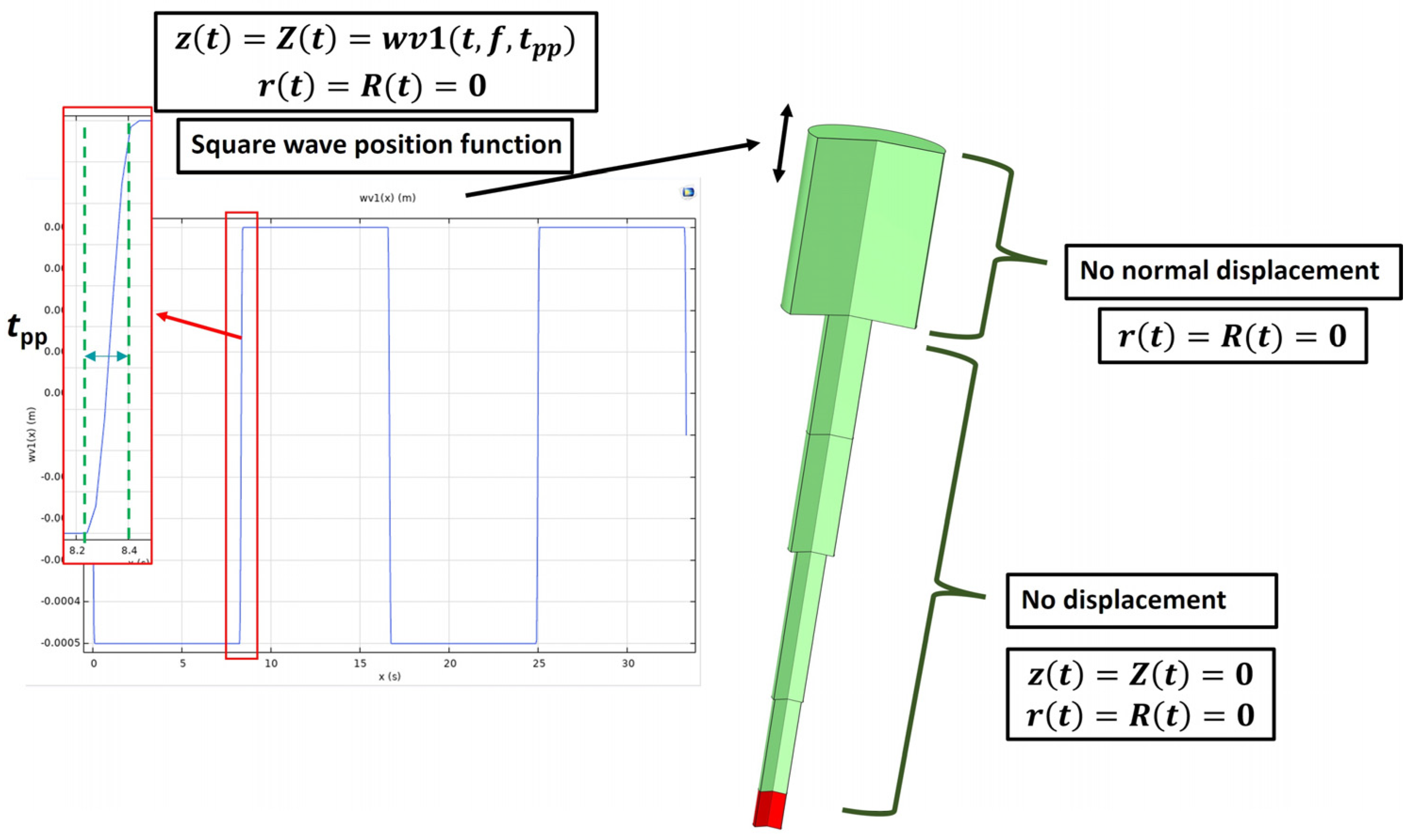
• On the top, the fluid velocity at the vertical direction, v_z, is equal to the velocity of the mechanical movement of the plate (see Figure 7):

  $$v_Z=\frac{\partial Z}{\partial t}=\frac{\partial z}{\partial t}$$

  (10)
• At the device walls, a “no slip” condition is forced; in other words, the velocity of the fluid at the walls is zero (see Figure 7):

  $$v=0$$

  (11)
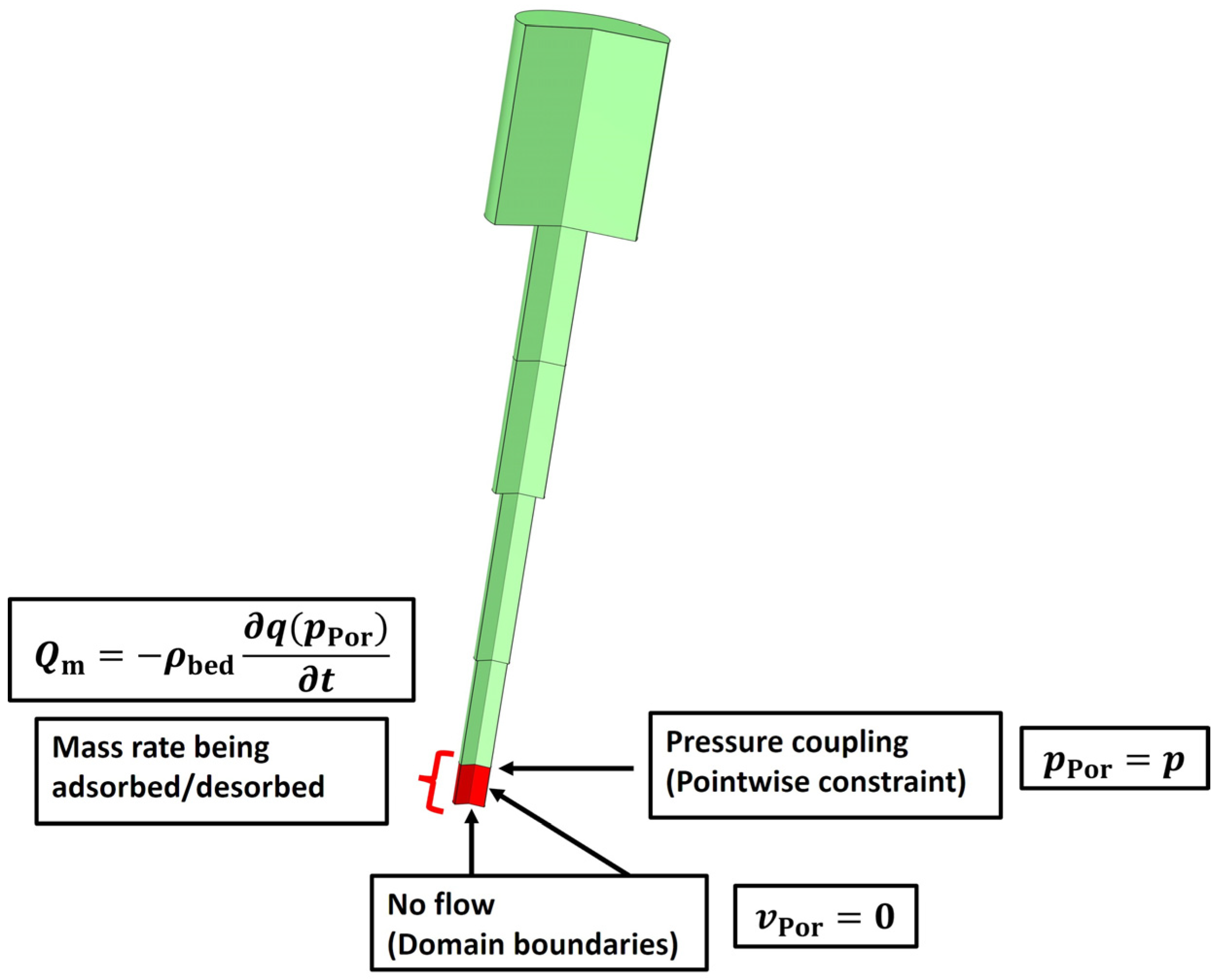
• In the general case, at the surface contact between the porous material and the gas, a coupling is completed between the CFD formulation and the Darcy’s Law physics module (suitable for low porosities). In this case, the so-called “leaking wall” boundary condition is used, where there is a fluid input or output coming from or flowing to the porous material. Under these circumstances, and as a coupling boundary condition with the porous media flow, the velocity of the gas at the wall is equal to the velocity of the fluid trespassing the barrier of the porous material, whose calculation will be detailed in the next subchapter, v_Por:

  $$\overrightarrow{v}=\overrightarrow{v_{\mathrm{Por}}}$$

  (12)

In this domain, a pressure probe is also defined to simulate the behavior of a real pressure sensor. This allows for a direct comparison of the experimental results with the simulated ones.

2.1.3. Porous Media Flow Simulation and Adsorption/Desorption Coupling

The remaining simulated physics (as mentioned in Section 2.1) correspond to the fluid transport through the porous material. For this case, there are two modeling options: Darcy’s Law or the Brinkman equations [55,66,67,68]. This depends on the conditions of the porous material.

Darcy’s Law is a commonly used formulation for underground filtering of fluids, whose main characteristic is a slow flow through low-porosity substrates [55,66]. On the other hand, the Brinkman equations are used for intermediate velocities between low-porosity material and free flow [67,68]. This corresponds to high-porosity beds, typically on the range of porosities higher than 0.5–0.6 in the case of a Stokes flow (higher otherwise) [56,69,70,71], where the porosity, ε_P, is the volume of the bed pores, V_Pores, (for instance, pores or empty spaces of a bed in a bed reactor) with respect to the total volume of the porous material (for instance, the volume of the bed) V_Total:

$${\epsilon }_{\mathrm{P}}=\frac{V_{\mathrm{Pores}}}{V_{\mathrm{Total}}}$$

(13)

If the Brinkman equations are used, the following set of equations, a modification of the Navier–Stokes (the Stokes formulation, which can be used in lower porosity beds), are solved:

$$\left\{\begin{array}{c}\frac{\partial {\epsilon }_{\mathrm{P}}\rho }{\partial t}+\overrightarrow{\nabla }\left(\rho \overrightarrow{v_{\mathrm{Por}}}\right)=Q_{\mathrm{m}}\\ \rho \frac{\partial \overrightarrow{v_{\mathrm{Por}}}}{\partial t}=\overrightarrow{\nabla }\left(-p_{\mathrm{Por}}I+\frac{\mu }{{\epsilon }_{\mathrm{P}}}\left(\nabla \overrightarrow{v_{\mathrm{Por}}}+{\left(\nabla \overrightarrow{v_{\mathrm{Por}}}\right)}^{\mathrm{T}}\right)-\frac{2}{3}\frac{\mu }{{\epsilon }_{\mathrm{P}}}\left(\nabla \overrightarrow{v_{\mathrm{Por}}}\right)I\right)-\left(\frac{\mu }{\kappa }+\frac{Q_{\mathrm{m}}}{{\epsilon }_{\mathrm{P}}{}^2}\right)\overrightarrow{v_{\mathrm{Por}}}\end{array}\right.$$

(14)

where ρ is the gas density, v_Por is the effective fluid velocity within the porous material, p_Por is the effective pressure within the porous material, κ is the permeability, and Q_m is the mass rate per volume unit, in kg/(m³s) from a mass source or sink.

In the case of low porosity, Darcy’s Law is used with the following formulation:

$$\left\{\begin{array}{c}\frac{\partial {\epsilon }_{\mathrm{P}}\rho }{\partial t}+\overrightarrow{\nabla }\left(\rho \overrightarrow{v_{\mathrm{Por}}}\right)=Q_{\mathrm{m}}\\ \overrightarrow{v_{\mathrm{Por}}}=-\frac{\kappa }{\mu }\overrightarrow{\nabla }{p}_{\mathrm{Por}}\end{array}\right.$$

(15)

It is noteworthy that Equations (14) and (15) do not need to be corrected with the ALE formulation. The reason is that the domains where these equations are applied do not have any frame movement.

The coupling between the free flow and the porous media flow must be defined at the boundary between them (the top surface of the bed of the porous material). The velocity condition in Equation (12) represents the coupling condition from the perspective of free-flow physics. Conversely, the other dependent variable must be coupled from the point of view of the porous media flow, which is the pressure, enforcing the following boundary condition (see Figure 8 and Figure 9):

$$p_{\mathrm{Por}}=p$$

(16)

Other domain boundaries are defined with a standard no-flow condition (see Figure 8):

$$v_{\mathrm{Por}}=0$$

(17)

The last term to define is the mass rate per volume unit, Q_m. From the fluid perspective, Q_m is the mass rate per volume unit that the fluid gains under a desorption process. Likewise, it is the mass rate per volume unit of the fluid that is lost if there is an adsorption process. This is calculated from the corresponding adsorption isotherm. As the system is assumed to be isothermal, if q(p) is the adsorption isotherm of a certain porous material with respect to the corresponding equilibrium pressure, p, in kg of adsorbed gas per kg of bulk solid substance, the rate of adsorption or desorption of gas per unit mass of bulk solid substance due to pressure change would be given by ∂q/∂t. However, from the fluid perspective, the sign of such a derivation must be negative (adsorption, the fluid loses mass), and the mass production rate, Q_m, must be compatible with Equations (14) and (15), leading to its final expression (see Figure 8):

$$Q_{\mathrm{m}}=-{\rho }_{\mathrm{bed}}\frac{\partial q\left(p_{\mathrm{Por}}\right)}{\partial t}=-\frac{m_{\mathrm{Bulk}}}{V_{\mathrm{bed}}}\frac{\partial q\left(p_{\mathrm{Por}}\right)}{\partial t}$$

(18)

If the adsorption isotherm would come in other units, the corresponding transformations must be performed so that the final mass rate per volume unit refers to the correct quantities. Some adsorption models that may be used for the calculation of q are the Langmuir model, Freundlich model, Sips model, among others [72]. In this work, for every case, the employed model will be described.

A qualitative summary of the complete model and its interdependencies can be found in the workflow of Figure 9.

2.2. Simulated Zeolite Systems

For the analysis and verification of the proposed model, three different systems were selected: HZSM-5/propane, silicalite-1/methane, and silicalite-1/ethane. In every example, the known and fitted data will be detailed as well as the simulation assumptions. Due to the different data availability, the procedures are different.

2.2.1. Experimental Setup: HZSM-5/Propane

The HZSM-5/propane system was tested in the FR device of the Chair of Thermodynamics of the Technische Universität Dresden. Technical details can be found in the article of Grün et al. [24]. As detailed there, the volume variation signal is a square wave at different frequencies (see Figure 2). The sample material was HZSM-5 from EVONIK (trade name CPC SP1000, Si/Al ratio 25) and propane (purity 3.5) supplied by MESSER INDUSTRIEGASE GMBH. For this experiment, data were extracted at frequencies ranging from 0.001 Hz to 1 Hz.

The properties used for propane are based on an ideal gas formulation for the density–pressure–temperature relation as given by the software used, while the temperature-dependent viscosity is obtained from the built-in temperature-dependent relation given in COMSOL Multiphysics^®, the employed simulation program. The conditions of the experiment at equilibrium (plate at a neutral position) were 317.25 K and 2.13 kPa. The mass of the sample, distributed as a homogeneous bed at the bottom of the sample chamber, is 0.5244 g. The depth of the bed sample is 13 mm, resulting in a bed density, ρ_bed, of 401.85 kg/m³. The particle diameter of the HZSM-5 sample is around 315–400 μm. In the simulation, the particle size is assumed to be the average of that distribution: d_Par = 357.4 μm.

The chosen adsorption isotherm follows the Langmuir formulation, using data from the literature [73,74] with the following expression:

$$q=q_{\max }\frac{K_{\mathrm{L}}{p}_{\mathrm{Por}}}{\left(1+K_{\mathrm{L}}{p}_{\mathrm{Por}}\right)}$$

(19)

where q_max = 1.47 mol/kg is the maximum adsorption capacity and K_L = 1.0742 kPa⁻¹ is the Langmuir constant. In this case, being M_gas the molar mass of the employed gas, Equation (18) is modified to the following:

$$Q_{\mathrm{m}}=-{\rho }_{\mathrm{bed}}\frac{\partial }{\partial t}\left(M_{\mathrm{gas}}{q}_{\max }\frac{K_{\mathrm{L}}{p}_{\mathrm{Por}}}{\left(1+K_{\mathrm{L}}{p}_{\mathrm{Por}}\right)}\right)$$

(20)

In this simulation, the unknown variable to solve is the density of the dry particle from the porous material (particle mass divided by its volume, including pores and blisters), ρ_D. The rest of the unknown properties are inferred from that one, such as the bed porosity:

$${\epsilon }_{\mathrm{P}}=\frac{{\rho }_{\mathrm{D}}-{\rho }_{\mathrm{bed}}}{{\rho }_{\mathrm{D}}}$$

(21)

Then, with the porosity, the permeability κ can be calculated with the expression of Kozeny–Carman, which is appropriate for viscous flows and packed beds as is the case in these measurements [66,75,76]:

$$\kappa =\frac{d_{\mathrm{Par}}{}^2}{180}\frac{{\epsilon }_{\mathrm{P}}{}^3}{\left(1-{\epsilon }_{\mathrm{P}}{}^2\right)}$$

(22)

The last step before performing the simulations is to make a volume correction. The simulation geometry (see Figure 3) only takes into account the geometry of the volume modulation unit. However, it does not consider the volume of other pipes that are attached to the volume modulation unit, whose size contributes to the total volume of the system. The distribution and orientation, mostly horizontal, of those additional pipes would break the axial symmetry of the model. Due to this fact, either the total volume of the simulation or the movement of the plate must be corrected to represent the same effects as in the real system. For that, the variation of pressure and variation of volume (see Figure 10) from the real system are inspected. The ideal gas equation is then employed for an estimation of the real overall volume and the correction needed in the simulation.

If an isothermal case is assumed, the ideal gas takes the following form:

$$pV=\mathrm{const}.$$

(23)

For the first variation of volume and pressure, the expression (23) can be transformed into the following:

$$pV=\left(p+\mathsf{\Delta }p\right)\left(V-\mathsf{\Delta }V\right)$$

(24)

Thus, the relation of the volume, V, and the variation of volume, ∆V, in the real system or in the simulation, should be the same to generate the experimental pressure result of the blank measurement (see Figure 10b) according to the following:

$$\frac{V}{\mathsf{\Delta }V}=\left(\frac{p}{\mathsf{\Delta }p}+1\right)$$

(25)

In the real system, the movement of the plate corresponds to ±0.5 mm, which with a plate diameter of 46 mm results in a volume change of ±830.951 mm³. Applying expression (25), the obtained real volume is about 785 cm³. If the simulation volume is 125.3 cm³, the movement of the plate in the simulation must be downscaled to ±0.079814 mm in order to simulate the effects of the real system. With these parameters, the simulated blank measurement is similar to the real one as shown in Figure 11.

2.2.2. Silicalite-1/Methane System

In this system, the model is compared to the single-step frequency response experiment of Van-Den-Begin et al. [21]. With the provided data, it is possible to compare the continuous measurement of the pressure change of the silicalite-1/methane system. The conditions of the experiment at equilibrium were 197 K and 15.15 Torr for the loaded device, while for the blank measurement, the pressure was reduced to 15.05 Torr.

The properties used for methane, as in the previous approach, are based on an ideal gas formulation for the density–pressure–temperature relation. The temperature-dependent viscosity is obtained from the tabular values contained in the reference thermophysical properties given in the NIST database [77].

Regarding the volume, it is known that the volume of the FR device is 100 cm³ with a volume modulation of ±1%. However, as it is a single-step frequency response method, and after checking the variation of volume with the blank measurement (see Figure 12), each step is given by a 2% volume variation. A comparison between the model and the experimental blank measurement was also performed. After inspecting the comparison in Figure 12, a correction of the simulation volume is not necessary. However, the geometry is not completely known and, as a consequence, a cylindrical structure of 20 cm² as a base, compatible with the built 2D-axilsymmetric model, is assumed for the simulation.

The particle radius of the employed silicalite-1 sample is known: 31 μm. For other properties, fixed values are not given, only a set of ranges where the values should be. For instance, the mass of the sample is between 0.05 and 0.3 g. The peak-to-peak time, t_pp, is between 25 and 35 ms. The particle dry density takes the typical value for silicalite-1 of ρ_D = 1760 kg/m³.

For this system, the chosen adsorption isotherm follows again the Langmuir formulation. After fitting the data from the literature [78] for a temperature of 197 K, the following expression is used:

$$q=q_{\max }\frac{K_{\mathrm{L}}{p}_{\mathrm{Por}}}{\left(1+K_{\mathrm{L}}{p}_{\mathrm{Por}}\right)}$$

(26)

where q_max = 335.31 cm³ STP/g is the maximum adsorption capacity and K_L = 2.807 bar⁻¹ is the Langmuir constant. The molar mass of the employed gas being M_gas, and after the transformation of q_max to mol/g, the following is derived:

$$Q_{\mathrm{m}}=-{\rho }_{\mathrm{bed}}\frac{\partial }{\partial t}\left(M_{\mathrm{gas}}{q}_{\max }\frac{K_{\mathrm{L}}{p}_{\mathrm{Por}}}{\left(1+K_{\mathrm{L}}{p}_{\mathrm{Por}}\right)}\right)$$

(27)

The fitting strategy is different in comparison to the previous system. The mass of the sample and the bed porosity are the unknowns that must be fitted against the pressure curves found in the literature. When both values are found, the bed porosity can be calculated as follows:

$${\rho }_{\mathrm{bed}}={\rho }_{\mathrm{D}}\left(1-{\epsilon }_{\mathrm{P}}\right)$$

(28)

With the bed density, the volume of the bed can be also readily calculated:

$$V_{\mathrm{bed}}=\frac{m_{\mathrm{sample}}}{{\rho }_{\mathrm{bed}}}$$

(29)

The last needed parameter is the permeability κ, which can be calculated, like in the previous subsection, with the expression of Kozeny–Carman:

$$\kappa =\frac{d_{\mathrm{Par}}{}^2}{180}\frac{{\epsilon }_{\mathrm{P}}{}^3}{\left(1-{\epsilon }_{\mathrm{P}}{}^2\right)}$$

(30)

This completes the set of parameters.

2.2.3. Silicalite-1/Ethane System

Analogously to the silicalite-1/methane system, the model is compared to the single-step frequency response experiment of Van-Den-Begin et al. [20]. The conditions of the experiment in the literature at equilibrium were 0 °C and 9.86 Torr for the loaded device. Unfortunately, no blank measurement was provided and thus the volume cannot be proved, only the volume variation (±1%). The volume, after some simulation testing, and within similar publications, will be assumed to be 202 cm³ with a surface cylindrical base of 12.6 cm² [54,79]. The bed depth should be around 1–5 mm.

For ethane, an ideal gas formulation for the density–pressure–temperature relation is employed. The reference thermophysical properties given in the NIST database [80] are used to define the temperature-dependent viscosity of ethane.

The silicalite-1 particle diameter is 14.4 μm, the mass of the sample is between 0.8 and 2.5 g, and the peak-to-peak time, t_pp, is between 25 and 35 ms. As in the previous case, the particle dry density takes the typical value for silicalite-1 of ρ_D = 1760 kg/m³.

The chosen adsorption isotherm model is the Toth model after fitting adsorption data from the literature [81]:

$$q=q_{\max }\frac{K_{\mathrm{T}}{p}_{\mathrm{Por}}}{{\left(1+{\left(K_{\mathrm{T}}{p}_{\mathrm{Por}}\right)}^{\raisebox{1ex}{$1$}\!\left/ \!\raisebox{-1ex}{$n$}\right.}\right)}^n},$$

(31)

where the fitted parameters are q_max = 1.9988 mmol/g, K_T = 0.01443 Torr⁻¹ (Toth constant), and n = 1.1904. M_gas being the molar mass of the used gas, the mass fluid production rate is the following:

$$Q_{\mathrm{m}}=-{\rho }_{\mathrm{bed}}\frac{\partial }{\partial t}\left(M_{\mathrm{gas}}{q}_{\max }\frac{K_{\mathrm{T}}{p}_{\mathrm{Por}}}{{\left(1+{\left(K_{\mathrm{T}}{p}_{\mathrm{Por}}\right)}^{\raisebox{1ex}{$1$}\!\left/ \!\raisebox{-1ex}{$n$}\right.}\right)}^n}\right)$$

(32)

In this example, the fitting strategy is the same as the one presented in Section 2.2.2. Consequently, the bed porosity, the bed volume, and the permeability are calculated using the same equations:

$${\rho }_{\mathrm{bed}}={\rho }_{\mathrm{D}}\left(1-{\epsilon }_{\mathrm{P}}\right)$$

(33)

$$V_{\mathrm{bed}}=\frac{m_{\mathrm{sample}}}{{\rho }_{\mathrm{bed}}}$$

(34)

$$\kappa =\frac{d_{\mathrm{Par}}{}^2}{180}\frac{{\epsilon }_{\mathrm{P}}{}^3}{\left(1-{\epsilon }_{\mathrm{P}}{}^2\right)}$$

(35)

However, there is a notable difference in the model. For this certain system, the porosity was found to be much higher than in the previous examples; in fact, it was found to be equal to or higher than 0.5. For this reason, instead of using Equation (15) for Darcy’s Law, the Brinkman Equation (14) is solved.

Due to the different datasets and particularities of the analyzed data, the model could be tested against a relatively wide range of usage scenarios, showing the versatility of the simulation, whose results are shown in Section 3.

2.3. Simulation Details

In this section, an overview of the characteristics of the simulation, including solvers or mesh sizes, will be provided. The first step is to conduct a mesh convergence analysis. The most relevant simulation parameters are related to the pressure response, as this parameter can be compared with the experimental data. Two values are considered for comparison: the peak relative pressure and the relative pressure at equilibrium. In the case of the system described in Section 2.2.1, this refers to the pressure just before a new plate movement. For the other two cases, it refers to the pressure in equilibrium after a sufficiently long time. The different meshes were evaluated based on the number of elements. Convergence is reached when the variation of the last two tested meshes is lower than 1%

The system described in Section 2.2.1. was evaluated at a frequency of 0.004 Hz. The results can be inspected in Figure 13. The variation between the last three tested meshes is less than 0.5%. The final mesh, consisting of 1257 elements, is displayed in Figure 14. The mesh base is an unstructured triangular mesh. Additional mesh refinement and three boundary layers are applied to the domains adjacent to the contact between the fluid flow and the porous medium. Three boundary layers are also included at the walls with a no-slip condition in order to better resolve the flow near the wall.

A similar study was conducted for the cylindrical geometry required for the silicalite-1/methane system. The plate’s movement mimics a single-step frequency response. Therefore, the equilibrium relative pressure is reached at the end of the simulation when it stabilizes. The result can be observed in Figure 15. Similar to the previous system, the variation between the last three tested meshes is less than 0.5%. The final mesh consists of 3773 structured quad elements (see Figure 16). A finer mesh is employed near the interface between the free flow and the porous flow.

The silicalite-1/ethane system also utilizes the single-step frequency response method, and thus, similar meshing principles are applied. The final mesh is displayed in Figure 17. It predominantly consists of a structured quad mesh, with the addition of boundary layers specific to the porous media domain (Figure 17b, at the bottom). This mesh comprises 5526 elements.

The next aspect to consider is time discretization. These simulations use an implicit time-dependent solver based on the Backward Differentiation Formula (BDF) solver [28,82,83] with “free time-stepping”. In this approach, the algorithm autonomously determines the appropriate time step in each iteration. The time step is successively reduced until the solver tolerance is met, which in this case is set at an absolute tolerance of 0.001. However, it is not advisable to rely solely on the solver’s discretion. Therefore, a maximum time step has been defined.

In the case of the experimental HZSM-5/propane system, which employs a square wave input at a specific frequency, the period T_F = 1/f serves as a reference. The maximum time step (t_s,max) is defined as follows:

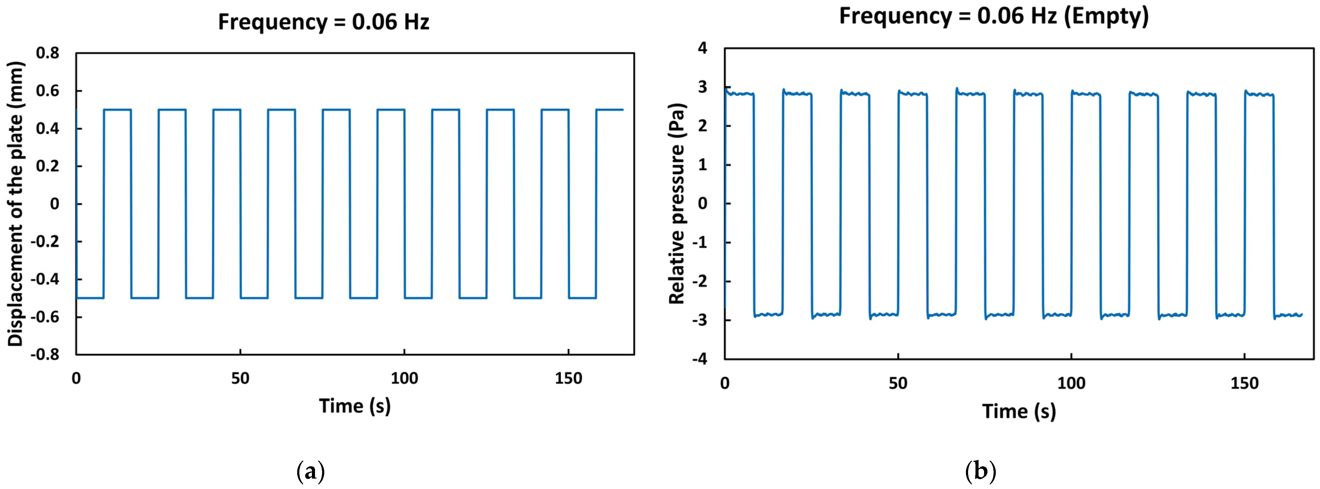
• t_s,max = 0.001T_F if this value is at least one order of magnitude lower than t_pp. Here, t_pp represents the rate of the plate movement, indicating how rapidly it changes position. This scenario is the most common one.
• If the previous condition is not met, especially during transitions from compression to expansion and vice versa, the maximum time step is progressively reduced one order of magnitude until it is at least one order of magnitude lower than t_pp. If every cycle is characterized by T_F, during the simulation time intervals of 0–1% T_F (part of the initial compression), 49–51% T_F (change from compression to expansion), and 99-100%T_F (part of the compression for the next cycle), t_s,max will be reduced to 0.0001T_F or even lower. This adjustment was only applicable at the studied frequency of 0.06 Hz. To compensate the additional time steps, t_s,max is increased to 0.01T_F for the ranges that were not mentioned. This should potentially compensate the overall number of computed points.

To validate the effectiveness of this approach, measurements of peak relative pressures and relative equilibrium pressures were taken and compared. For the second approach, involving a frequency of 0.06 Hz, the measured values were 2.8583 Pa and 1.9940 Pa for peak relative pressures and relative equilibrium pressures, respectively. After increasing the maximum time step by ten times under all conditions, the resulting values were 2.8598 Pa and 1.9939 Pa for peak relative pressures and relative equilibrium pressures, respectively. The difference observed is below 0.1%, demonstrating the success of this strategy.

In the case of the other two systems, a maximum time step of 0.0001s was defined, which was consistently one or two orders of magnitude lower than t_pp.

Regarding the coupling solving strategy, two options exist: monolithic and partitioned [84,85,86,87]. In the partitioned or segregated approach [85], each physics is solved independently from the others. The modeler must specify the order in which the physics are solved in each time step. After solving the first subdomain, the results at the boundaries are transferred to the next subdomain. An advantage of this approach is that each physics can use highly optimized, independent solvers. However, with each time step, a small error is introduced due to the partial decoupling, which can lead to non-convergent solutions after a certain number of time steps. In contrast, the monolithic or fully coupled approach [84,87] solves all physics and variables simultaneously in each time step. This approach is generally more accurate but also more computationally expensive, as it requires the simultaneous discretization and solution of all physics. This monolithic approach is the one employed in this work.

As monolithic approaches can suffer from ill-conditioning, a suitable combination is to use a direct solver. Direct solvers are more robust and can handle ill-conditioned problems better compared to iterative solvers [88,89], which often require extensive fine-tuning [88,90]. Direct solvers solve the system of equations through a straightforward, “brute force” approach. While they offer advantages in terms of robustness, fine-tuned iterative solvers are generally faster. Given the number of equations and physics involved in this work, the MUMPS direct solver [91,92] is used for the simulations. Quadratic Lagrange shape functions are selected for all dependent variables except for the pressure of the free flow, whose shape function is linear. Additionally, it is worth noting that before conducting the time-dependent simulations, a stationary pre-step is performed to establish a stable initial state for the system before the plate movement commences.

3. Results and Discussion

In this section, the simulation results will be evaluated. The structure of the presentation of the results will be similar to that of the Section 2. Each zeolite/gas system will be introduced, the fitted parameters as well as the simulation results will be shown and interpreted, and, depending on the case, a study of the influencing parameters will be performed.

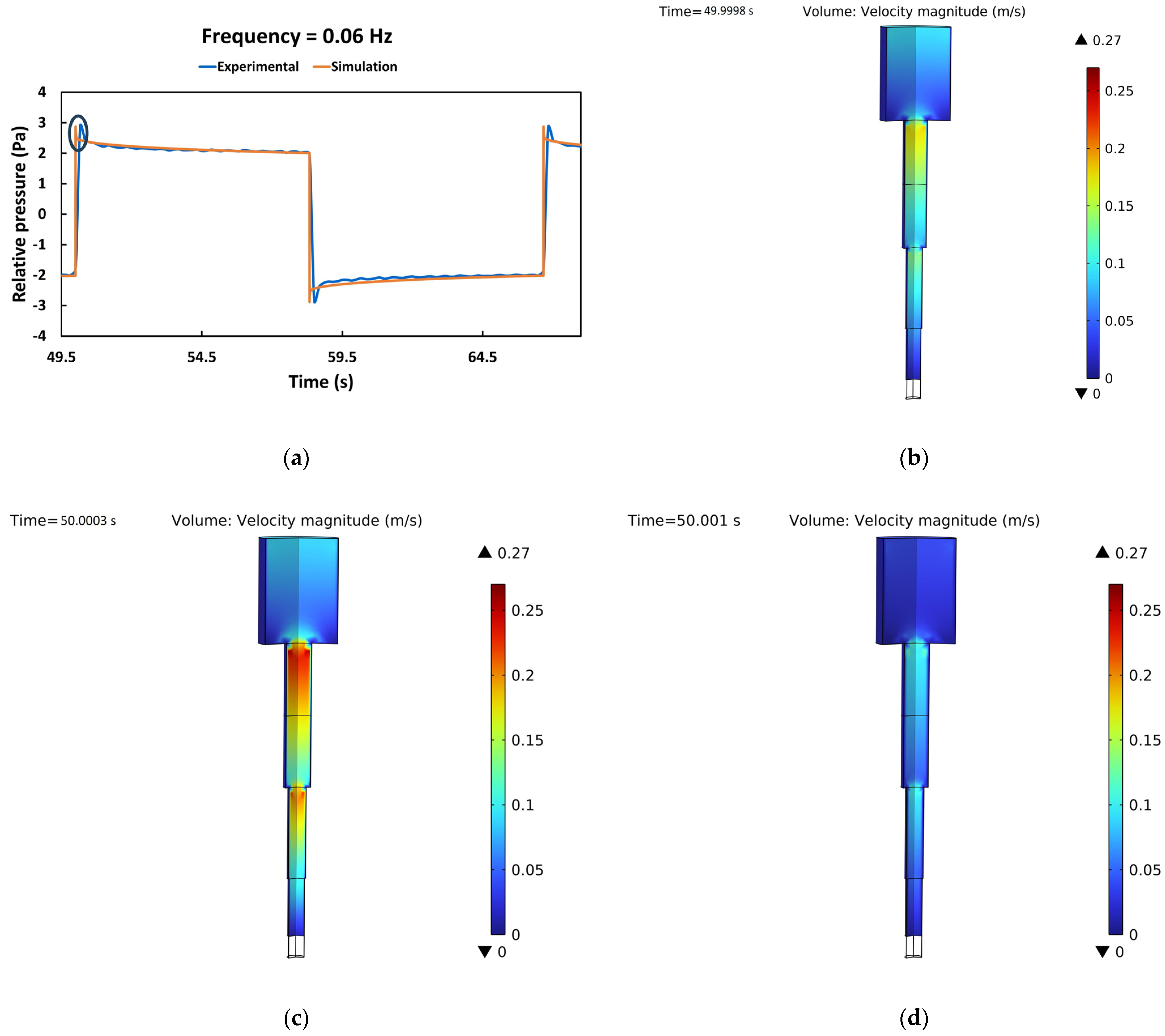
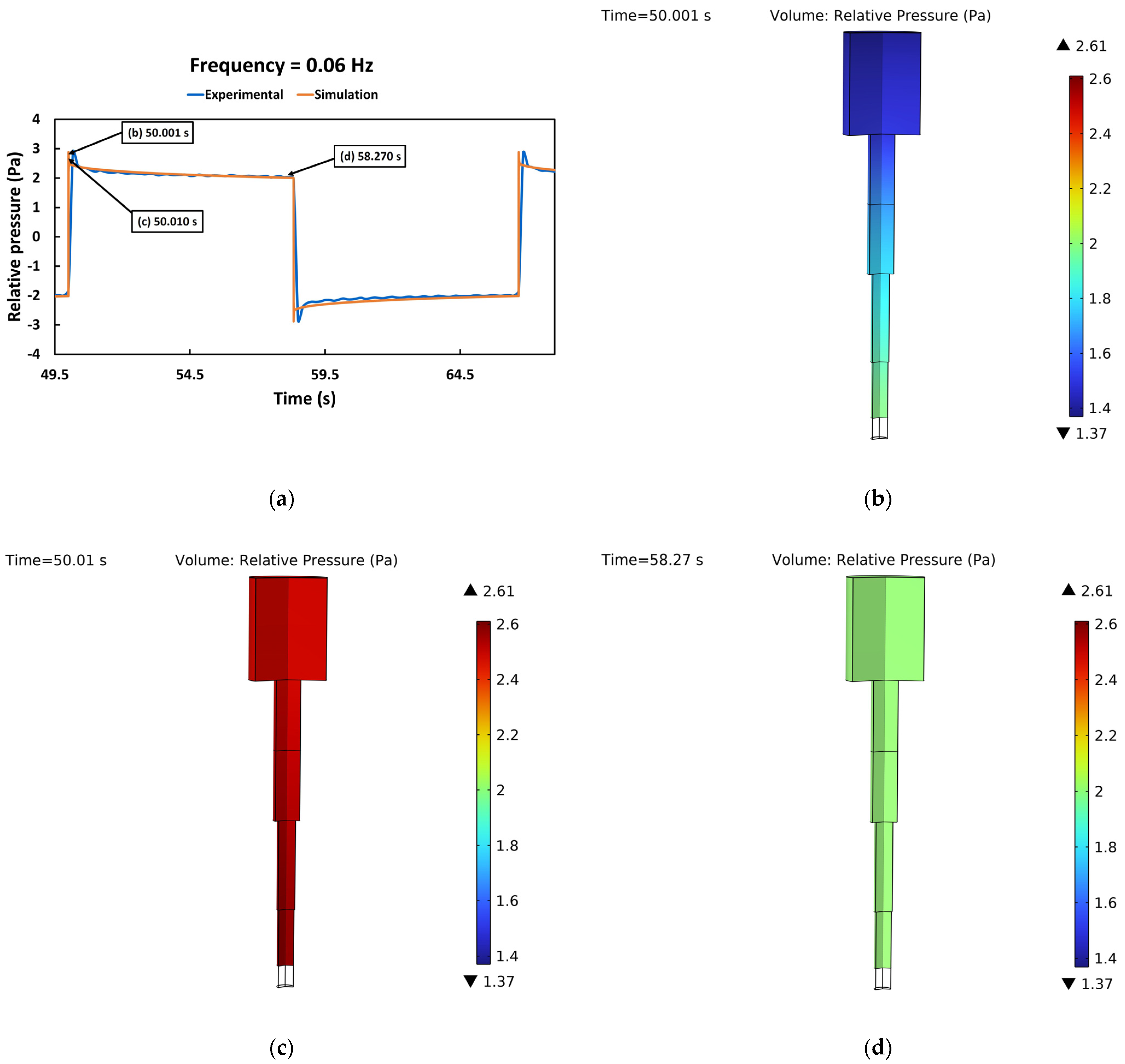
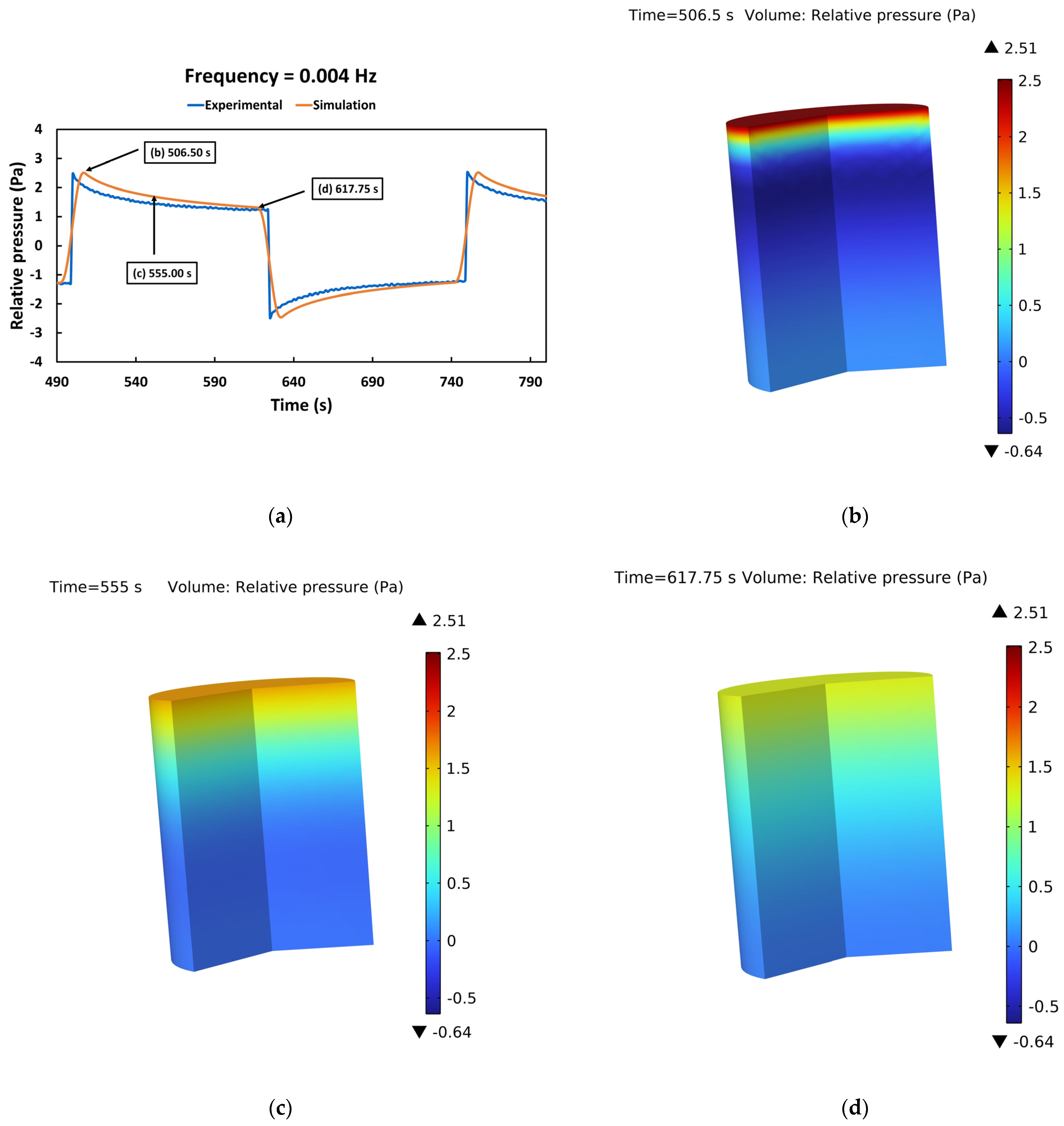
3.1. Experimental Setup: HZSM-5/Propane

This system was analyzed at various frequencies ranging from 0.001 Hz to 1 Hz. Out of these frequencies, four scenarios were arbitrarily selected to assess the ability of the model to replicate the experimental behavior. Relative lower frequencies were preferred due to their resemblance to the single-step frequency response used in the other two systems. The chosen frequencies were 0.002 Hz, 0.004 Hz, 0.008 Hz, and 0.06 Hz.

Table 1. Fitted data for the simulation of the HZSM-5/propane system at the different chosen frequency levels.

Experimental Frequency	0.002 Hz	0.004 Hz	0.008 Hz	0.06 Hz
Particle dry density, ρD	419.93 kg/m3	421.94 kg/m3	423.95 kg/m3	417.92 kg/m3
Bed porosity, εP	0.0431	0.0476	0.0521	0.0385
Time peak-to-peak, tpp	45 s	17 s	6.5 s	3.2 ms

shows the fitted data based on the assumptions and models explained in Section 2.2.1. The curve fitting process involves comparing the pressure level points just before a new semicycle (i.e., the transition from compression to expansion) and the peak values of the experimental data with their counterparts in the simulation. An alternative approach could be to fit the entire curve using the least-squares method. However, this would significantly increase simulation times due to the large number of comparison points and the numerous simulations required to fit the data at multiple frequencies. Our current comparison is primarily for an initial model evaluation.

For less extensive datasets (like in Section 3.2 and Section 3.3), the least-squares method was, conversely, employed.

Table 1 reveals that the fitted particle dry density remains relatively consistent across all four datasets with only a minor variation of 1–2%. This slight variation in particle dry density leads to a significantly higher deviation in bed porosity when using Equation (21). Upon closer examination of the porosity values, they share a similar order of magnitude, all falling well below 0.5. This suggests that the Darcy’s Law model is applicable to all cases. However, the porosity values do exhibit oscillations, ranging from 0.0385 to 0.0521. Such fluctuations are relatively high, considering that porosity is a key parameter influencing the shape of the pressure curve. Consequently, when using the suggested simulation method with an unknown porosity, it can only provide an estimated range of values.

The last parameter in Table 1 is the fitted peak-to-peak time of the simulated volume modulation curve. These times have a notable impact on the peaks of the pressure curve in simulations. They appear to scale inversely with the experimental frequency. This inverse relationship may be attributed to the consistent number of sampled experimental points, which is typically around 1000 points for five or ten oscillations, regardless of the chosen frequency. Consequently, changes in the sampling frequency scale proportionally with the experimental frequency. This results in the smoothing out of real high-frequency peaks when operating at low frequencies, as the electromagnetic actuator has, from its specifications, lower peak-to-peak times (around the order of milliseconds) compared to the values listed in Table 1.

As will be shown in Section 3.2, peak-to-peak times primarily affect the highest peaks and have a minimal impact on the pressure decay curve. Therefore, the experimental peaks were just used for fitting this specific parameter. Additionally, there appears to be an outlier in the measurement at 0.06 Hz, where exceptionally high peak values were recorded. This anomaly suggests that some sampled points in this experiment were arbitrarily registered on that particular peak, resembling the operational range of the magnetic actuator, which operates on the order of milliseconds, as mentioned previously.

The results of the simulations compared to the measured experimental data are shown in Figure 18. The model’s performance shows a slight improvement as the frequency increases. Given certain unknowns, such as the actual adsorption/desorption behavior of the system (various adsorption/desorption curves exist in the literature), it is anticipated that the simulation results may not perfectly match the experimental curves. Nevertheless, they exhibit a high degree of qualitative similarity with only minor differences. In the worst-case scenario, the disparity between the experimental and simulation data is approximately 0.3 Pa. This discrepancy is deemed acceptable, considering the likelihood of additional system effects beyond those considered in the model.

In addition to the comparative diagrams, the model developed in COMSOL Multiphysics^® offers several advantages over conventional methods. It has the capability to visualize local effects within different domains of the simulation. The model allows the tracking of how the pressure, velocity, and amount of adsorbed gas evolve through the various system domains over time. Specifically, Figure 19 and Figure 20 illustrate the speed and pressure distribution within the volume devoid of porous material at different simulation times for the experiment at 0.06 Hz. Figure 19 focuses on the variation of the flow velocity during the compression step of the moving plate. Figure 19b depicts a point in the middle of the compression step. The velocity field can be seen around the plate area due to the plate’s action. As the fluid is pushed downwards, the velocity increases as the diameter decreases (this is expected). Figure 19c shows a higher flow speed after more time under the effect of the moving plate, while Figure 19d shows a decrease in flow speed shortly after the movement of the plate stops.

The pressure distribution can be observed in Figure 20 at three different points on the curve. The greatest pressure differences can be observed in Figure 20b, which corresponds to the end of the plate displacement. Around the point of the end of the plate movement, with some pressure oscillations, there is a greater pressure gradient compared to Figure 20c, which represents the beginning of the relaxing cycle after the oscillations, or Figure 20d, where the system is almost in equilibrium.

Concerning the porous material region, some simulation results are displayed in Figure 21 (adsorption rate) and Figure 22 (pressure distribution) at 0.004 Hz. Progressing from Figure 21b to Figure 21d, the adsorption front becomes evident. As the system approaches equilibrium, the adsorption rate decreases while the adsorption front descends. This showcases the kinetic evolution of the adsorption process and the resistance to the flow of the porous material. This pattern is also confirmed in Figure 22. Transitioning from Figure 22b to Figure 22d, the decrease in the pressure gradient is noticeable as it tends towards equilibrium, making it more challenging for the gas to flow through the porous material.

For enhanced visualization, Video S1, Video S2, and Video S3 (fixed color legend) or Video S4, Video S5, and Video S6 (dynamic color legend) are provided in the Supplementary Materials. These videos allow the observation of the comprehensive simulation of the relative pressure distribution in the domain without porous material, the relative pressure distribution within the porous material bed, and the adsorbed gas rate within the porous material bed, respectively, all pertaining to the 0.004 Hz frequency.

The 3D view of the simulation offers a means to visualize internal local variations within the system and track the evolution of the adsorption front. Moreover, this model is versatile and can accommodate heterogeneous structures, such as systems with two distinct porous materials, allowing for a localized assessment of each porous material’s contribution. An alternative application involves defining various diffusion effects when multiple channel structures exist, such as adsorption occurring in macropores and micropores. This can be achieved by specifying simultaneous sources or sinks of gas within the porous material, denoted by the term Q_m in (14) or (15).

3.2. Silicalite-1/Methane System

The following system corresponds to the data from the literature provided by Van-Den-Begin et al. [21], where a single-step frequency response is employed. The known parameters were already presented in Section 2.2.2. The data were fitted against the overall pressure curve by a standard least-squares, adjusting each fitted simulation parameter iteratively. The outcomes of this fitting procedure are presented in

Table 2. Fitted data for the simulation of the silicalite-1/methane system with the single-step frequency response.

Mass, msample	Bed Density, ρbed	Bed Porosity, εP	Time Peak-to-Peak, tpp
0.116 g	1601.6 kg/m3	0.09	28 ms

.

The result of the simulation in comparison to the experimental points can be found in Figure 23. The results are very similar to the experimental values with all the points within a difference of 0.02 Torr (largest deviation) and a relative error of 0.13% or lower. This shows the suitability of the model to represent such forms of FR analysis.

For this specific comparison, a small parameter analysis was conducted to partially investigate the model dependencies and their impact on the simulation output. This information is useful for verifying if the physics of the model align with expectations. The tested parameters include geometrical changes to the chamber, the mass of the sample, bed porosity, and the peak-to-peak times. Parameters not mentioned in each specific case stayed as listed in Table 2.

Regarding the geometrical features, two different base areas and bed depths were tested with the same volume (100 cm³) and cylindrical structure. In the first case, the geometry had a base surface of 20 cm², resulting in a bed depth of 36.21 μm. In the second case, the base surface was 5 cm², causing a bed depth of and 144.86 μm. The first bed depth is too small, even lower than the particle diameter. This is likely due to the initial estimated geometry of the system, which may have overestimated the diameter. The results are displayed in Figure 24a, clearly showing that the model can capture the bed effects arising from different bed depths. These bed effects are highly noticeable and can significantly alter the results. Therefore, precise geometrical details of the sample chamber and bed depth are crucial for this model.

An advantage of this model is its capacity to distinguish bed effects from adsorption effects, a feat that other analytical characteristic methods may struggle with or require complex mathematical adjustments [93,94]. An interesting observation is that varying bed depths, while keeping the sample mass constant, does not alter the final equilibrium pressure (see Figure 24a). This is logical since the same mass of porous material can adsorb the same amount of gas regardless of bed depth, albeit with similar volume/pressure variations. The difference in the pressure curve decay arises from the accessibility to the solid surface, with higher bed depths offering more resistance to porous flow and thereby reducing the velocity of the adsorption process, as seen in Figure 24a.

Concerning the mass of the sample, two values were tested: 0.116 g and 0.300 g. The comparison is presented in Figure 24b. In this case, there is a significant variation in the final equilibrium pressure. This is expected as a higher mass can absorb larger amounts of gas. Kinetically, there are also some differences to consider: the gas has to diffuse through a larger amount of porous material, provoking an increase in bed depth to 93.66 μm when the rest of the simulation parameters are constant. As a consequence, the increase in sample mass produces a decrease in the overall process speed.

In Figure 24c, two pressure curves at different bed porosities (0.09 and 0.12) are compared. Since there is no variation in zeolite mass, the final equilibrium pressure value remains the same for both simulations. However, the increase in bed porosity, although it slightly increases the bed depth (ρ_bed = 1548.8 kg/m³, bed depth of 37.45 μm), leads to an acceleration in the decay rate of the pressure curve. In other words, the gas can flow faster through the macropores of the particle bed and the gas can be adsorbed more rapidly. This is a result of reduced flow resistance, allowing the gas to contact a greater solid surface area in a shorter period of time. This adjustment also affects the peak of the pressure curve.

The final comparison is performed with different peak-to-peak times of the movement of the plate. Figure 24d shows the comparison between 28 ms and 5 ms. The results indicate minimal changes in the curves: the final equilibrium pressure remains identical, and the slope of the pressure decay is also similar. The only discernible difference is in the peak pressure value, which is attributed to the higher initial flow speed and its impact when the gas first reaches the surface of the porous material. This effect is more pronounced at higher modulation speeds. Nevertheless, it does not significantly influence the rest of the adsorption/desorption process, although it could impact curve analysis in some analytical approaches where peak characteristics are integral to the fitting procedure.

With these results, the model has been validated using external data, successfully replicating values from the literature despite uncertainties about the geometry of the FR device. A parameter analysis was performed and the decoupling between the transport phenomena through the bed of particles and the adsorption/desorption phenomena was proved. Following this system, further validation of the model was undertaken with a different gas and solid combination.

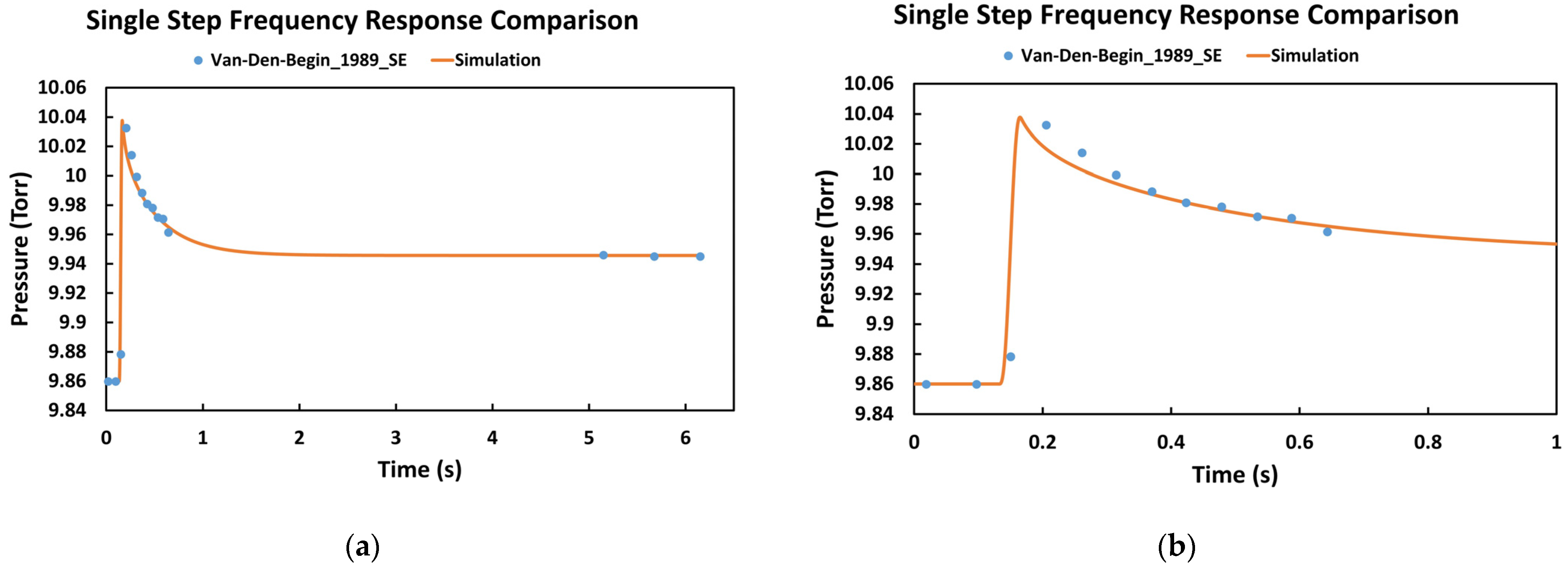
3.3. Silicalite-1/Ethane System

The third tested case corresponds to the system composed of silicalite-1 and ethane. The employed literature data are sourced from the work of Van-Den-Begin et al. [20]. In this case, a single-step frequency response is used, which is similar to the silicalite-1/methane system. Since the model’s behavior should align with the parameter variations discussed in Section 3.2, only a direct comparison of the literature data was performed. In Section 2.2.3, the known parameters of the system were previously introduced. The fitted data, using a standard least-squares method against the literature curve, are given in

Table 3. Fitted data for the simulation of the silicalite-1/ethane system with the single-step frequency response.

Mass, msample	Bed Density, ρbed	Bed Porosity, εP	Time Peak-to-Peak, tpp
0.81 g	880 kg/m3	0.5	35 ms

.

The fitted data presented in Table 2 falls within the range of values found in the literature. It is worth noting that the estimated bed depth in the literature was between 1 and 5 mm, while the obtained bed depth in the simulation was 0.75 mm. The most probable reason of this discrepancy is the difference in geometry between the real and simulated case, especially considering the lack of specific details about the shape of the real structure, as mentioned in Section 2.2.3. The result of the simulation in comparison to the experimental points is displayed in Figure 25. The difference in the simulation and data from the literature is lower than 0.015 Torr (worst case) or lower than 0.15%.

This last validation case shows that the model can accurately represent this type of data within a satisfactory precision range. It is essential to acknowledge that there are numerous uncertainties associated with this validation, primarily stemming from the lack of detailed information about the geometrical structure of the system and the provided experimental details. Nevertheless, the model capabilities were proved for the frequency response experimental data, as well as for single-step frequency response analysis. This showcases the appropriateness of the chosen physics incorporated into the model and underscores its ability to effectively decouple transport phenomena from adsorption phenomena. Furthermore, the presented model can be used for unknown data fitting or potentially for analysis of experimental data deviation and its possible causes.

4. Conclusions

The presented COMSOL Multiphysics^® model simulates the frequency response phenomena by effectively separating the transport phenomena and adsorption phenomena. For the transport aspect, computational fluid dynamics is utilized to describe gas transport within the empty FR device. For adsorption phenomena, a porous media flow based on Darcy’s Law, or the Brinkman equations if the bed porosity is relatively large, is employed for the effective gas flow in the porous material. In this work, the studied porous materials consisted of MFI zeolites (HZSM-5 or silicalite-1). The adsorption/desorption of gas is modeled through a mass sink or source, respectively, based on the change in gas adsorption equilibrium provided by the adsorption isotherm of the studied system. A dynamic change in pressure provokes a change in the mass adsorption rate according to the corresponding adsorption isotherm model. With this approach, the transport and adsorption can be successfully decoupled.

To better understand the model’s behavior, a small parameter variation study was performed by changing the mass of the porous material, the bed porosity, the peak-to-peak time variation, and the geometry of the system. It was revealed that the geometry of the device, which indirectly affects the bed depth of the porous material, exerts a significant influence on the results. Higher bed depths introduce greater resistance to fluid flow, affecting the kinetics of the process by reducing the process speed. The mass of the sample had the highest influence on the final equilibrium pressure. When the mass remained constant within the same system, the final equilibrium pressure remained unchanged. Bed porosity also influences the kinetics. In general, higher porosity facilitated gas flow, resulting in a faster pressure response within the system. Lastly, the peak-to-peak time only affected the initial pressure peak, probably due to the first impact against the porous material surface.

Following the fitting of unknown system parameters, the model consistently yielded satisfactory results, typically within a single-digit percentage difference, especially against the pressure values found in the literature. This validation affirms the model’s suitability under various working conditions and confirms the reliability of the underlying physics. However, it is essential to exercise caution concerning several factors, including the geometric features of the real system (and the potential need for simulated volume corrections), the chosen adsorption model, accurate material parameters, and precise bed characteristics. These considerations are critical to ensure the model’s accuracy and reliability.

The presented model has the capacity to fit unknown data, such as bed porosity and adsorption isotherms. Additionally, it provides the capability for a detailed local examination of system variables within the porous material, including parameters like pressure, flow velocity, or the gas adsorption rate. Potentially, it can be used to uncover discrepancies in experimental data or identify non-linearities, especially in more complex models. While not explicitly tested in this work, the model may also be employed to study multiple spatially separated porous materials within a single system or to explore the combination of different adsorption and desorption mechanisms.

In conclusion, the introduced simulation model provides a valuable additional tool to evaluate zeolites or other porous material/gas systems, which can be combined with other analytical approaches to obtain deeper information about the diffusion capabilities of the studied system.

References

1. Karge, H.G.; Weitkamp, J. Zeolites as Catalysts, Sorbents and Detergent Builders: Applications and Innovations; Elsevier: Amsterdam, The Netherlands, 1989; ISBN 978-0-08-088741-8. [Google Scholar]
2. Karge, H.G.; Weitkamp, J. (Eds.) Adsorption and Diffusion; Molecular Sieves; Springer: Berlin/Heidelberg, Germany, 2008; ISBN 978-3-540-73965-4. [Google Scholar]
3. Gleaves, J.T.; Ebner, J.R.; Kuechler, T.C. Temporal Analysis of Products (TAP)—A Unique Catalyst Evaluation System with Submillisecond Time Resolution. Catal. Rev. 1988, 30, 49–116. [Google Scholar] [CrossRef]
4. Breitkopf, C. An Integrated Catalytic and Transient Study of Sulfated Zirconias: Investigation of the Reaction Mechanism and the Role of Acidic Sites in n-Butane Isomerization. ChemCatChem 2009, 1, 259–269. [Google Scholar] [CrossRef]
5. Breitkopf, C. Spezielle labortechnische Reaktoren: TAP-Reaktor. In Handbuch Chemische Reaktoren: Chemische Reaktionstechnik: Theoretische und Praktische Grundlagen, Chemische Reaktionsapparate in Theorie und Praxis; Reschetilowski, W., Ed.; Springer Reference Naturwissenschaften; Springer: Berlin, Heidelberg, 2020; pp. 1321–1360. ISBN 978-3-662-56434-9. [Google Scholar]
6. Breitkopf, C.; Swider-Lyons, K. (Eds.) Springer Handbook of Electrochemical Energy; Springer: Berlin/Heidelberg, Germany, 2017; ISBN 978-3-662-46656-8. [Google Scholar]
7. Nguyen, T.Q.; Breitkopf, C. Determination of Diffusion Coefficients Using Impedance Spectroscopy Data. J. Electrochem. Soc. 2018, 165, E826–E831. [Google Scholar] [CrossRef]
8. Yasuda, Y. Determination of Vapor Diffusion Coefficients in Zeolite by the Frequency Response Method. J. Phys. Chem. 1982, 86, 1913–1917. [Google Scholar] [CrossRef]
9. Shen, D.; Rees, L.V.C. Diffusivities of Benzene in HZSM-5, Silicalite-I, and NaX Determined by Frequency-Response Techniques. Zeolites 1991, 11, 666–671. [Google Scholar] [CrossRef]
10. Reyes, S.C.; Sinfelt, J.H.; DeMartin, G.J.; Ernst, R.H.; Iglesia, E. Frequency Modulation Methods for Diffusion and Adsorption Measurements in Porous Solids. J. Phys. Chem. B 1997, 101, 614–622. [Google Scholar] [CrossRef]
11. Naphtali, L.M.; Polinski, L.M. A Novel Technique for Characterization of Adsorption Rates on Heterogeneous Surfaces. J. Phys. Chem. 1963, 67, 369–375. [Google Scholar] [CrossRef]
12. Yasuda, Y. Frequency Response Method for Study of the Kinetic Behavior of a Gas-Surface System. 1. Theoretical Treatment. J. Phys. Chem. 1976, 80, 1867–1869. [Google Scholar] [CrossRef]
13. Yasuda, Y. Frequency Response Method for Study of the Kinetic Behavior of a Gas-Surface System. 2. An Ethylene-on-Zinc Oxide System. J. Phys. Chem. 1976, 80, 1870–1875. [Google Scholar] [CrossRef]
14. Song, L.; Rees, L.V. Frequency Response Measurements of Diffusion in Microporous Materials. In Adsorption and Diffusion; Springer: Berlin/Heidelberg, Germany, 2007; pp. 235–276. [Google Scholar]
15. Song, L.; Rees, L.V.C. Adsorption and Transport of N-Hexane in Silicalite-1 by the Frequency Response Technique. Faraday Trans. 1997, 93, 649–657. [Google Scholar] [CrossRef]
16. Yasuda, Y.; Suzuki, Y.; Fukada, H. Kinetic Details of a Gas/Porous Adsorbent System by the Frequency Response Method. J. Phys. Chem. 1991, 95, 2486–2492. [Google Scholar] [CrossRef]
17. Jordi, R.G.; Do, D.D. Frequency-Response Analysis of Sorption in Zeolite Crystals with Finite Intracrystal Reversible Mass Exchange. J. Chem. Soc. Faraday Trans. 1992, 88, 2411–2419. [Google Scholar] [CrossRef]
18. Rees, L.V.C.; Shen, D. Characterization of Microporous Sorbents by Frequency-Response Methods. Gas Sep. Purif. 1993, 7, 83–89. [Google Scholar] [CrossRef]
19. Bourdin, V.; Gray, P.G.; Grenier, P.; Terrier, M.F. An Apparatus for Adsorption Dynamics Studies Using Infrared Measurement of the Adsorbent Temperature. Rev. Sci. Instrum. 1998, 69, 2130–2136. [Google Scholar] [CrossRef]
20. Van-Den-Begin, N.; Rees, L.V.C.; Caro, J.; Bülow, M.; Hunger, M.; Kärger, J. Diffusion of Ethane in Silicalite-1 by Frequency Response, Sorption Uptake and Nuclear Magnetic Resonance Techniques. J. Chem. Soc. Faraday Trans. 1989, 85, 1501–1509. [Google Scholar] [CrossRef]
21. Van-Den-Begin, N.; Rees, L.V.C.; Caro, J.; Bülow, M. Fast Adsorption-Desorption Kinetics of Hydrocarbons in Silicalite-1 by the Single-Step Frequency Response Method. Zeolites 1989, 9, 287–292. [Google Scholar] [CrossRef]
22. Song, L.; Rees, L.V.C. Adsorption and Diffusion of Cyclic Hydrocarbon in MFI-Type Zeolites Studied by Gravimetric and Frequency-Response Techniques. Microporous Mesoporous Mater. 2000, 35, 301–314. [Google Scholar] [CrossRef]
23. Valyon, J.; Onyestyák, G.; Rees, L.V.C. A Frequency-Response Study of the Diffusion and Sorption Dynamics of Ammonia in Zeolites. Langmuir 2000, 16, 1331–1336. [Google Scholar] [CrossRef]
24. Grün, R.; Pan, F.; Grau Turuelo, C.; Breitkopf, C. Transient Studies of Gas Transport in Porous Solids Using Frequency Response Method—A Conceptual Study. Catal. Today 2023, 417, 113838. [Google Scholar] [CrossRef]
25. Stein, E.; Borst, R.d.; Hughes, T.J.R. Encyclopedia of Computational Mechanics Volume 1 Fundamentals, Part 1, 2nd ed.; Wiley: Chichester, UK, 2018. [Google Scholar] [CrossRef]
26. Bosma, T. Levelset Based Fluid-Structure Interaction Modeling with the eXtended Finite Element Method. Master’s Thesis, Delft University of Technology, Delft, The Netherlands, 2013. [Google Scholar]
27. Bruchon, J.; Digonnet, H.; Coupez, T. Using a Signed Distance Function for the Simulation of Metal Forming Processes: Formulation of the Contact Condition and Mesh Adaptation. From a Lagrangian Approach to an Eulerian Approach. Int. J. Numer. Methods Eng. 2009, 78, 980–1008. [Google Scholar] [CrossRef]
28. COMSOL. Multiphysics Reference Manual, Version 6.1, COMSOL, Inc. Available online: www.comsol.com (accessed on 15 July 2023).
29. Rao, K.S.; Sravani, K.G.; Yugandhar, G.; Rao, G.V.; Mani, V.N. Design and Analysis of Fluid Structure Interaction in a Horizontal Micro Channel. Procedia Mater. Sci. 2015, 10, 768–788. [Google Scholar] [CrossRef]
30. Maruthavanan, D.; Seibel, A.; Schlattmann, J. Fluid-Structure Interaction Modelling of a Soft Pneumatic Actuator. Actuators 2021, 10, 163. [Google Scholar] [CrossRef]
31. Silva, K.E.S.; Sivapuram, R.; Ranjbarzadeh, S.; Gioria, R.S.; Silva, E.C.N.; Picelli, R. Topology Optimization of Stationary Fluid–Structure Interaction Problems Including Large Displacements via the TOBS-GT Method. Struct. Multidiscip. Optim. 2022, 65, 337. [Google Scholar] [CrossRef]
32. Ivanov, A.; Kovacs, A.; Mescheder, U. High Quality 3D Shapes by Silicon Anodization. Phys. Status Solidi A 2011, 208, 1383–1388. [Google Scholar] [CrossRef]
33. Smallwood, D.C.; McCloskey, P.; Rohan, J.F. Multiphysics Design and Fabrication of 3D Electroplated VIA Materials Topographies for next Generation Energy and Sensor Technologies. Mater. Des. 2022, 221, 111001. [Google Scholar] [CrossRef]
34. Waltz, J.; Morgan, N.R.; Canfield, T.R.; Charest, M.R.J.; Risinger, L.D.; Wohlbier, J.G. A Three-Dimensional Finite Element Arbitrary Lagrangian–Eulerian Method for Shock Hydrodynamics on Unstructured Grids. Comput. Fluids 2014, 92, 172–187. [Google Scholar] [CrossRef]
35. Löhner, R.; Yang, C. Improved ALE Mesh Velocities for Moving Bodies. Commun. Numer. Methods Eng. 1996, 12, 599–608. [Google Scholar] [CrossRef]
36. Zreid, I.; Behnke, R.; Kaliske, M. ALE Formulation for Thermomechanical Inelastic Material Models Applied to Tire Forming and Curing Simulations. Comput. Mech. 2021, 67, 1543–1557. [Google Scholar] [CrossRef]
37. Lin, P.T.; Baker, T.J.; Martinelli, L.; Jameson, A. Two-Dimensional Implicit Time-Dependent Calculations on Adaptive Unstructured Meshes with Time Evolving Boundaries. Int. J. Numer. Methods Fluids 2006, 50, 199–218. [Google Scholar] [CrossRef]
38. Filipovic, N.; Mijailovic, S.; Tsuda, A.; Kojic, M. An Implicit Algorithm within the Arbitrary Lagrangian–Eulerian Formulation for Solving Incompressible Fluid Flow with Large Boundary Motions. Comput. Methods Appl. Mech. Eng. 2006, 195, 6347–6361. [Google Scholar] [CrossRef]
39. Winslow, A.M. “‘Equipotential’” Zoning of Two-Dimensional Meshes; California University, Lawrence Livermore Lab: Livermore, CA, USA, 1963. [Google Scholar]
40. Winslow, A.M. Numerical Solution of the Quasilinear Poisson Equation in a Nonuniform Triangle Mesh. J. Comput. Phys. 1966, 1, 149–172. [Google Scholar] [CrossRef]
41. Winslow, A.M.; Barton, R.T. Rescaling of Equipotential Smoothing; Lawrence Livermore National Lab. (LLNL): Livermore, CA, USA, 1982. [Google Scholar]
42. Donea, J.; Huerta, A.; Ponthot, J.-P.; Rodríguez-Ferran, A. Arbitrary Lagrangian–Eulerian Methods. In Encyclopedia of Computational Mechanics; John Wiley & Sons, Ltd.: Hoboken, NJ, USA, 2004; ISBN 978-0-470-09135-7. [Google Scholar]
43. Maire, P.-H.; De Buhan, M.; Diaz, A.; Dobrzynski, C.; Kluth, G.; Lagoutière, F. A Cell-Centered Arbitrary Lagrangian Eulerian (ALE) Method for Multi-Material Compressible Flows. ESAIM: Proc. 2008, 24, 1–13. [Google Scholar] [CrossRef]
44. Liu, W.K.; Chen, J.-S.; Belytschko, T.; Zhang, Y.F. Adaptive ALE Finite Elements with Particular Reference to External Work Rate on Frictional Interface. Comput. Methods Appl. Mech. Eng. 1991, 93, 189–216. [Google Scholar] [CrossRef]
45. Mokbel, M.; Aland, S. An ALE Method for Simulations of Axisymmetric Elastic Surfaces in Flow. Int. J. Numer. Methods Fluids 2020, 92, 1604–1625. [Google Scholar] [CrossRef]
46. Matsushima, K.; Murayama, M.; Nakahashi, K. Unstructured Dynamic Mesh for Large Movement and Deformation. In Proceedings of the 40th AIAA Aerospace Sciences Meeting & Exhibit; Aerospace Sciences Meetings, Reno, NV, USA, 14–17 January 2002. [Google Scholar]
47. Tonon, P.; Sanches, R.A.K.; Takizawa, K.; Tezduyar, T.E. A Linear-Elasticity-Based Mesh Moving Method with No Cycle-to-Cycle Accumulated Distortion. Comput. Mech. 2021, 67, 413–434. [Google Scholar] [CrossRef]
48. Stein, K.; Tezduyar, T. Advanced Mesh Update Techniques for Problems Involving Large Displacements. In Proceedings of the Fifth World Congress on Computational Mechanics, Wienna, Austria, 7–12 July 2002. [Google Scholar]
49. Stein, K.; Tezduyar, T.; Benney, R. Mesh Moving Techniques for Fluid-Structure Interactions With Large Displacements. J. Appl. Mech. 2003, 70, 58–63. [Google Scholar] [CrossRef]
50. Rodríguez-Ferran, A.; Pérez-Foguet, A.; Huerta, A. Arbitrary Lagrangian-Eulerian (ALE) Formulation for Hyperelastoplasticity. Int. J. Numer. Methods Eng. 2002, 53, 1831–1851. [Google Scholar] [CrossRef]
51. Yamada, T.; Kikuchi, F. An Arbitrary Lagrangian-Eulerian Finite Element Method for Incompressible Hyperelasticity. Comput. Methods Appl. Mech. Eng. 1993, 102, 149–177. [Google Scholar] [CrossRef]
52. Renaud, C.; Cros, J.-M.; Feng, Z.-Q.; Yang, B. The Yeoh Model Applied to the Modeling of Large Deformation Contact/Impact Problems. Int. J. Impact Eng. 2009, 36, 659–666. [Google Scholar] [CrossRef]
53. Hossain, M.I.; Holland, C.E.; Ebner, A.D.; Ritter, J.A. 110th Anniversary: New Volumetric Frequency Response System for Determining Mass Transfer Mechanisms in Microporous Adsorbents. Ind. Eng. Chem. Res. 2019, 58, 17462–17474. [Google Scholar] [CrossRef]
54. Van-Den-Begin, N.G.; Rees, L.V.C. Diffusion of Hydrocarbons in Silicalite Using a Frequency-Response Method. In Studies in Surface Science and Catalysis; Elsevier: Amsterdam, The Netherlands, 1989; Volume 49, pp. 915–924. ISBN 978-0-444-87466-5. [Google Scholar]
55. Bear, J. Hydraulics of Groundwater; Courier Corporation: Chelmsford, MA, USA, 2012; ISBN 978-0-486-13616-5. [Google Scholar]
56. Kim, S.; Russel, W.B. Modelling of Porous Media by Renormalization of the Stokes Equations. J. Fluid Mech. 1985, 154, 269–286. [Google Scholar] [CrossRef]
57. Stewart, J. Calculus: Early Transcendentals; Textbooks Available with Cengage Youbook; Cengage Learning: Boston, MA, USA, 2010; ISBN 978-0-538-49790-9. [Google Scholar]
58. Liu, X.; Gui, N.; Wu, H.; Yang, X.; Tu, J.; Jiang, S. Numerical Simulation of Flow Past Stationary and Oscillating Deformable Circles with Fluid-Structure Interaction. Exp. Comput. Multiph. Flow 2020, 2, 151–161. [Google Scholar] [CrossRef]
59. Duarte, F.; Gormaz, R.; Natesan, S. Arbitrary Lagrangian–Eulerian Method for Navier–Stokes Equations with Moving Boundaries. Comput. Methods Appl. Mech. Eng. 2004, 193, 4819–4836. [Google Scholar] [CrossRef]
60. Liu, W.K.; Herman, C.; Jiun-Shyan, C.; Ted, B. Arbitrary Lagrangian-Eulerian Petrov-Galerkin Finite Elements for Nonlinear Continua. Comput. Methods Appl. Mech. Eng. 1988, 68, 259–310. [Google Scholar] [CrossRef]
61. Donea, J.; Giuliani, S.; Halleux, J.P. An Arbitrary Lagrangian-Eulerian Finite Element Method for Transient Dynamic Fluid-Structure Interactions. Comput. Methods Appl. Mech. Eng. 1982, 33, 689–723. [Google Scholar] [CrossRef]
62. Benson, D.J. An Efficient, Accurate, Simple Ale Method for Nonlinear Finite Element Programs. Comput. Methods Appl. Mech. Eng. 1989, 72, 305–350. [Google Scholar] [CrossRef]
63. Stokes, G.G. (Ed.) On the Theories of the Internal Friction of Fluids in Motion, and of the Equilibrium and Motion of Elastic Solids. In Mathematical and Physical Papers; Cambridge Library Collection—Mathematics; Cambridge University Press: Cambridge, UK, 2009; Volume 1, pp. 75–129. ISBN 978-1-108-00262-2. [Google Scholar]
64. Kim, S.; Karrila, S.J. Microhydrodynamics: Principles and Selected Applications; Courier Corporation: Boston, MA, USA, 2013. [Google Scholar]
65. Happel, J.; Brenner, H. Low Reynolds Number Hydrodynamics: With Special Applications to Particulate Media; Mechanics of Fluids and Transport Processes; Springer Netherlands: Dordrecht, The Netherlands, 1983; Volume 1, ISBN 978-90-247-2877-0. [Google Scholar]
66. Bear, J. Dynamics of Fluids in Porous Media; Courier Corporation: Boston, MA, USA, 2013; ISBN 978-0-486-13180-1. [Google Scholar]
67. Le Bars, M.; Worster, M.G. Interfacial Conditions between a Pure Fluid and a Porous Medium: Implications for Binary Alloy Solidification. J. Fluid Mech. 2006, 550, 149–173. [Google Scholar] [CrossRef]
68. Nield, D.A.; Bejan, A. Convection in Porous Media; Springer International Publishing: Cham, Switzerland, 2017; ISBN 978-3-319-49561-3. [Google Scholar]
69. Nield, D.A. The Limitations of the Brinkman-Forchheimer Equation in Modeling Flow in a Saturated Porous Medium and at an Interface. Int. J. Heat Fluid Flow 1991, 12, 269–272. [Google Scholar] [CrossRef]
70. Lundgren, T.S. Slow Flow through Stationary Random Beds and Suspensions of Spheres. J. Fluid Mech. 1972, 51, 273–299. [Google Scholar] [CrossRef]
71. Durlofsky, L.; Brady, J.F. Analysis of the Brinkman Equation as a Model for Flow in Porous Media. Phys. Fluids 1987, 30, 3329–3341. [Google Scholar] [CrossRef]
72. Kalam, S.; Abu-Khamsin, S.A.; Kamal, M.S.; Patil, S. Surfactant Adsorption Isotherms: A Review. ACS Omega 2021, 6, 32342–32348. [Google Scholar] [CrossRef] [PubMed]
73. Eder, F.; Stockenhuber, M.; Lercher, J.A. Sorption of Light Alkanes on H-ZSM5 and H-Mordenite. Stud. Surf. Sci. Catal. 1995, 97, 495–500. [Google Scholar] [CrossRef]
74. Eder, F.; Lercher, J.A. On the Role of the Pore Size and Tortuosity for Sorption of Alkanes in Molecular Sieves. J. Phys. Chem. B 1997, 101, 1273–1278. [Google Scholar] [CrossRef]
75. Carman, P.C. Flow of Gases through Porous Media; Butterworths Scientific Publications: London, UK, 1956. [Google Scholar]
76. Carman, P.C. Fluid Flow through Granular Beds. Chem. Eng. Res. Des. 1997, 75, S32–S48. [Google Scholar] [CrossRef]
77. Friend, D.G.; Ely, J.F.; Ingham, H. Thermophysical Properties of Methane. J. Phys. Chem. Ref. Data 1989, 18, 583–638. [Google Scholar] [CrossRef]
78. Yang, J.; Li, J.; Wang, W.; Li, L.; Li, J. Adsorption of CO2, CH4, and N2 on 8-, 10-, and 12-Membered Ring Hydrophobic Microporous High-Silica Zeolites: DDR, Silicalite-1, and Beta. Ind. Eng. Chem. Res. 2013, 52, 17856–17864. [Google Scholar] [CrossRef]
79. Karger, J.; Pfeifer, H.; Freude, D.; Caro, J.; Bulow, M.; Ohlmann, G. New Developments in Zeolite Science and Technology. In Surface Science and Catalysis, Proceedings of the 7th International Zeolite Conference, Tokyo, Japan, 17–22 August 1986; Kodansha: Tokyo, Japan; Elsevier: Amsterdam, The Netherlands, 1986; Volume 28, p. 633. [Google Scholar]
80. Friend, D.G.; Ingham, H.; Fly, J.F. Thermophysical Properties of Ethane. J. Phys. Chem. Ref. Data 1991, 20, 275–347. [Google Scholar] [CrossRef]
81. Dunne, J.A.; Mariwala, R.; Rao, M.; Sircar, S.; Gorte, R.J.; Myers, A.L. Calorimetric Heats of Adsorption and Adsorption Isotherms. 1. O2, N2, Ar, CO2, CH4, C2H6, and SF6 on Silicalite. Langmuir 1996, 12, 5888–5895. [Google Scholar] [CrossRef]
82. Hindmarsh, A.C.; Brown, P.N.; Grant, K.E.; Lee, S.L.; Serban, R.; Shumaker, D.E.; Woodward, C.S. SUNDIALS: Suite of Nonlinear and Differential/Algebraic Equation Solvers. ACM Trans. Math. Softw. 2005, 31, 363–396. [Google Scholar] [CrossRef]
83. Brown, P.N.; Hindmarsh, A.C.; Petzold, L.R. Using Krylov Methods in the Solution of Large-Scale Differential-Algebraic Systems. SIAM J. Sci. Comput. 1994, 15, 1467–1488. [Google Scholar] [CrossRef]
84. Zorrilla, R.; Rossi, R.; Wüchner, R.; Oñate, E. An Embedded Finite Element Framework for the Resolution of Strongly Coupled Fluid–Structure Interaction Problems. Application to Volumetric and Membrane-like Structures. Comput. Methods Appl. Mech. Eng. 2020, 368, 113179. [Google Scholar] [CrossRef]
85. Rossi, R.; Ryzhakov, P.B.; Oñate, E. A Monolithic FE Formulation for the Analysis of Membranes in Fluids. Int. J. Space Struct. 2009, 24, 205–210. [Google Scholar] [CrossRef]
86. Degroote, J.; Bathe, K.-J.; Vierendeels, J. Performance of a New Partitioned Procedure versus a Monolithic Procedure in Fluid–Structure Interaction. Comput. Struct. 2009, 87, 793–801. [Google Scholar] [CrossRef]
87. Failer, L.; Richter, T. A Parallel Newton Multigrid Framework for Monolithic Fluid-Structure Interactions. J. Sci. Comput. 2020, 82, 28. [Google Scholar] [CrossRef]
88. Langer, U.; Neumüller, M. Direct and Iterative Solvers. In Computational Acoustics; Kaltenbacher, M., Ed.; CISM International Centre for Mechanical Sciences; Springer International Publishing: Cham, Switzerland, 2018; Volume 579, pp. 205–251. ISBN 978-3-319-59037-0. [Google Scholar]
89. Press, W.H.; Flannery, B.P.; Teukolsky, S.A.; Vetterling, W.T. Numerical Recipes in FORTRAN 77: Volume 1, Volume 1 of Fortran Numerical Recipes: The Art of Scientific Computing; Cambridge University Press: Cambridge, UK, 1992; ISBN 978-0-521-43064-7. [Google Scholar]
90. Greenbaum, A. Iterative Methods for Solving Linear Systems; Society for Industrial and Applied Mathematics: Philadelphia, PA, USA, 1997. [Google Scholar] [CrossRef]
91. Amestoy, P.R.; Duff, I.S.; Koster, J.; L’Excellent, J.-Y. A Fully Asynchronous Multifrontal Solver Using Distributed Dynamic Scheduling. SIAM J. Matrix Anal. Appl. 2001, 23, 15–41. [Google Scholar] [CrossRef]
92. Amestoy, P.R.; Guermouche, A.; L’Excellent, J.-Y.; Pralet, S. Hybrid Scheduling for the Parallel Solution of Linear Systems. Parallel Comput. 2006, 32, 136–156. [Google Scholar] [CrossRef]
93. Crank, J. The Mathematics of Diffusion, 2d ed.; Clarendon Press: Oxford, UK, 1975; ISBN 978-0-19-853344-3. [Google Scholar]
94. Kärger, J.; Ruthven, D.M. Diffusion in Zeolites and Other Microporous Solids; Wiley: New York, NY, USA, 1992; ISBN 978-0-471-50907-3. [Google Scholar]
Figure 1. Qualitative FR characteristic out-of-phase function. Red: FR characteristic function of a single faster diffusion process with a diffusion coefficient of D = 10−13 m2s−1. Green: FR characteristic function of a single slower diffusion process with a diffusion coefficient of D = 10−15 m2s−1. Blue: FR characteristic function of a system with both diffusion processes.
Minerals 13 01238 g001
Figure 2. (a) Plate movement signal that produces the volume modulation at a frequency of 0.06 Hz and (b) relative pressure response of a performed loaded measurement at the same frequency [own apparatus].
Minerals 13 01238 g002
Figure 3. Simulated geometry and physics involved. Green: gas transport without porous material. Red: gas transport through the sample porous material coupled with adsorption/desorption.
Minerals 13 01238 g003
Figure 4. Dimensions of the simulated geometry.
Minerals 13 01238 g004
Figure 5. Boundary conditions of the deformed geometry formulation.
Minerals 13 01238 g005
Figure 6. (a) Mesh elements after compression (vertical displacement of –1 mm) and (b) mesh elements after expansion (vertical displacement of +1 mm). Red lines are the initial position of the geometry before the movement starts.
Minerals 13 01238 g006
Figure 7. Boundary conditions of the computational fluid dynamics interface.
Minerals 13 01238 g007
Figure 8. Boundary conditions and mass source/sink of the porous media flow formulation.
Minerals 13 01238 g008
Figure 9. Workflow of the described model. Orange: the four coupled physics; blue: the coupling conditions; green: the experimental data as input or as comparison point.
Minerals 13 01238 g009
Figure 10. (a) Plate displacement at a frequency of 0.06 Hz and (b) relative pressure response of the blank measurement at the same frequency [own apparatus].
Minerals 13 01238 g010
Figure 11. Comparison of the blank measurement [own apparatus] after the volume correction (only one cycle).
Minerals 13 01238 g011
Figure 12. Comparison of experimental literature data points (blue) from the blank measurements of Van-Den-Begin_SM [21] and simulated curves (orange) for (a) the highest variation area and (b) the final equilibrium pressure value.
Minerals 13 01238 g012
Figure 13. Mesh convergence study for the HZSM-5/propane system with respect to (a) the relative pressure before a new compression/expansion cycle begins and (b) the peak relative pressure.
Minerals 13 01238 g013
Figure 14. Final mesh distribution of the geometry simulated for the HZSM-5/propane system: (a) top part of the geometry and (b) bottom part of the geometry.
Minerals 13 01238 g014
Figure 15. Mesh convergence study for the silicalite-1/methane system with respect to (a) the final relative pressure and (b) the peak relative pressure.
Minerals 13 01238 g015
Figure 16. Final mesh distribution of the geometry simulated for the silicalite-1/methane system: (a) top part of the geometry and (b) bottom part of the geometry.
Minerals 13 01238 g016
Figure 17. Final mesh distribution of the geometry simulated for the silicalite-1/ethane system: (a) top part of the geometry and (b) bottom part of the geometry.
Minerals 13 01238 g017
Figure 18. Comparison of experimental curves (blue) [own apparatus] and simulated curves (orange) for (a) 0.002 Hz, (b) 0.004 Hz, (c) 0.008 Hz, (d) 0.06 Hz.
Minerals 13 01238 g018
Figure 19. A 3D view of the velocity field distribution at different simulation times in the domain without porous material for the experiment at 0.06 Hz. (a) Representation of one period and sampled zone for the simulation output shown from (b–d). Colors show the velocity values according to the color legend.
Minerals 13 01238 g019
Figure 20. A 3D view of the relative pressure distribution at different simulation times in the domain without porous material for the experiment at 0.06 Hz. (a) Representation of one period and taken simulation times for the simulation output shown from (b–d). Colors show the relative pressure values according to the color legend.
Minerals 13 01238 g020
Figure 21. A 3D view of the adsorbed gas rate at different simulation times within the porous material bed for the experiment at 0.004 Hz. (a) Representation of one period and taken simulation times for the simulation output shown from (b–d). Colors show the adsorbed gas rate values according to the color legend.
Minerals 13 01238 g021
Figure 22. A 3D view of the relative pressure distribution at different simulation times within the porous material bed for the experiment at 0.004 Hz. (a) Representation of one period and taken simulation times for the simulation output shown from (bd). Colors show the relative pressure values according to the color legend.
Minerals 13 01238 g022
Figure 23. Comparison of experimental literature points (blue) from Van-Den-Begin_SM [21] and simulated curves (orange) for (a) the highest variation area and (b) the final equilibrium pressure value.
Minerals 13 01238 g023
Figure 24. Variation of the pressure response under the effect of changes in different simulation parameters: (a) base of the cylindrical geometry and thus the bed depth; (b) mass of the sample msample; (c) bed porosity εP; (d) peak-to-peak time tpp.
Minerals 13 01238 g024
Figure 25. Comparison of experimental literature points (blue) from Van-Den-Begin_SE [20] and simulated curves (orange) for (a) the complete curve and (b) the highest variation part.
Minerals 13 01238 g025