Scale-Up Investigation of a Pilot and Industrial Scale Semi-Autogenous Mill Using a Particle Scale Model

Abstract

A particle scale model based on a full two-way coupling of the Discrete Element Method (DEM) and Smoothed Particle Hydrodynamics (SPHs) methods is applied to SAG mills. Motion and collisions of resolved coarser particles within an SAG mill are performed by the DEM component. Fine particles in the feed combine with the water to form a slurry, which is represented by the SPH component of the model. Slurry rheology is controlled by solid loading and fine particle size distribution for each volume of slurry. Transport, dispersion, and grinding of the slurry phase particle size distribution are predicted by solving additional coupled advection–diffusion equations in the SPH component of the model. Grinding of the finer particles in the slurry due to collisions and shear of the coarser particles (rocks and grinding media) is achieved via the inclusion of population balance terms in these equations for each SPH particle. This allows prediction of the transport of both coarser and finer material within the grinding and pulp chambers of an SAG mill, including the discharge performance of the mill. This particle-scale model is used to investigate the relative performance (throughput, product size distribution, resident particle size distribution, net power draw, wear) for an SAG mill at a pilot scale and a 36 ft industrial scale. The 36′ SAG mill considered is a geometrically scaled-up version of the 1.8 m Hardinge pilot scale mill but with a longer belly length, reflecting current SAG mill design preferences. The belly lifters are scaled to a lesser degree with a larger number of lifters used (but still many fewer liners than would typically be used in a large SAG mill based on conventional liner selection rules). The model shows that despite reasonable qualitative similarities, many aspects of the charge structure, slurry transport, coarse particle and slurry discharge through the grates, and the collision energy spectra vary in important ways. This demonstrates that a near purely geometric scale-up of an SAG mill is not sufficient to produce a comparable performance at the two physical mill scales.

1. Introduction

Semi-autogenous (SAG) mills are a broadly adopted class of comminution devices used for the large-scale grinding of rocks in mineral processing. Although geometrically fairly simple, they display a broad range of dynamics with complex interactions that make their selection, design, operation, and scale-up difficult. Economic drivers [1] motivate the ongoing need to better understand these machines to be able to improve their performance and predict their scale-up. Dunne et al. [2] make the economic benefit of using a larger SAG mill very clear, stating “economics dictated maximum throughput through a single line comminution circuit”. This paper also makes very clear the challenges of selecting the engineering the largest diameter SAG mill in the world at that time. The updated lists of installed mills provided at the 2011 and 2015 SAG conferences by Jones and Fresco [3] and Tozlu and Fresco [4] clearly demonstrate a trend towards larger SAG mills.

This paper offers designers an alternative path to progressing design changes in very small steps for the minimisation of risk. However, testing by simulation will also need to be supported by physical testing.

The Discrete Element Method (DEM) was originally developed for rock mechanics [5]. It has been used as a powerful tool for predicting dry charge motion in mills since Mishra and Rajamani [6,7] first developed models of 2D ball mills, and later to assess lifter designs for media overthrow in SAG mills [8]. Three-dimensional axial slice models of tumbling mills were used to study the effect of operating conditions on mill performance and wear prediction [9,10]. These models are useful for capturing many aspects of charge flow and power draw prediction but neglect the important effects of the mill end walls, slurry flow, axial segregation, and feed and discharge processes. Full 3D modelling of the pilot scale Hardinge mill was introduced by Morrison and Cleary [11]. A 3D DEM has since been adopted more broadly to investigate comminution fundamentals (such as energy utilisation for liberation), inform mill and liner design choices, and solve operational process issues [12,13,14,15,16,17,18,19]. For a general review of the DEM, see [20]. For a more detailed discussion of the leading edge of DEM development for comminution applications, see [21,22].

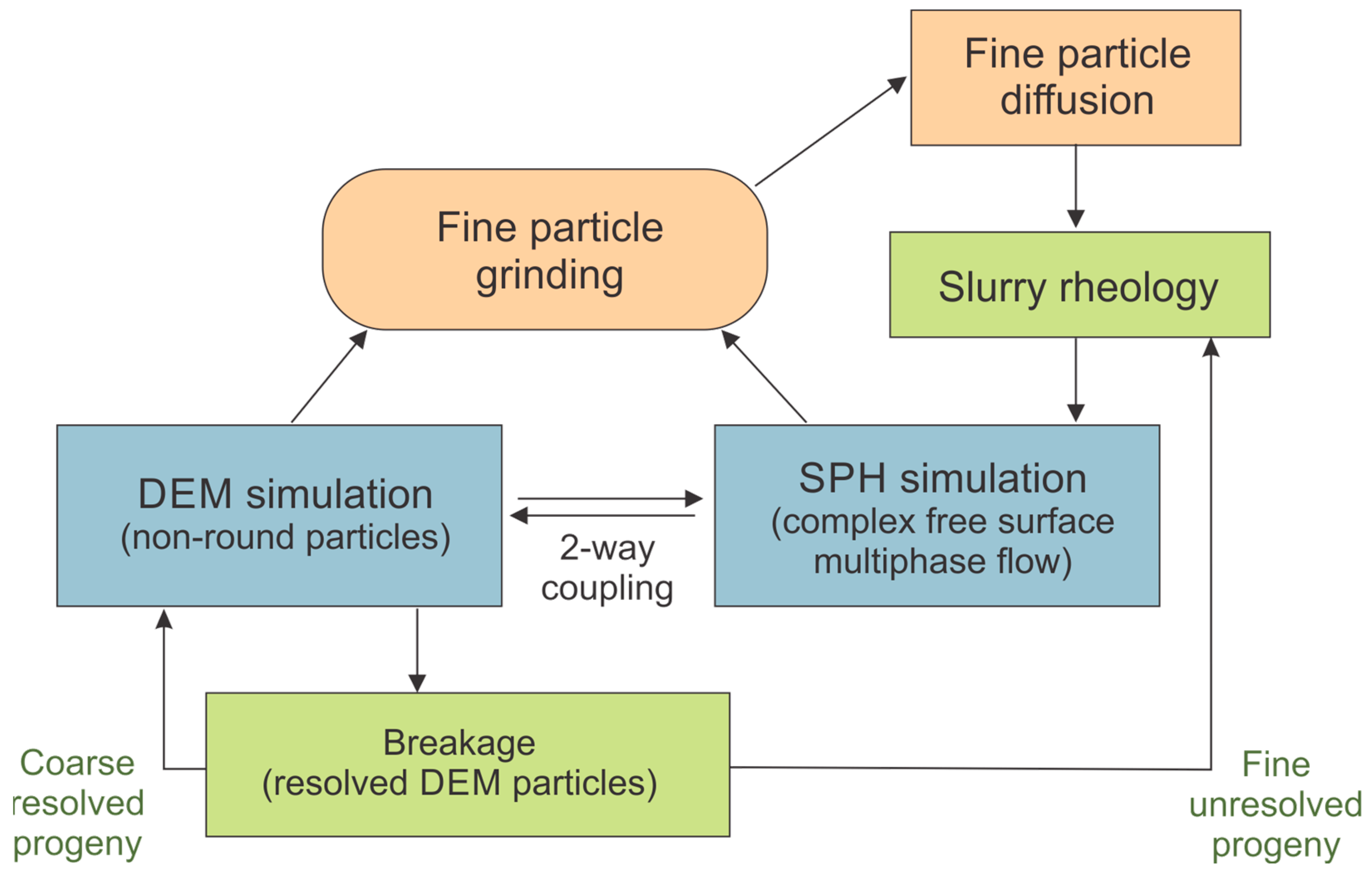
Slurry transport of finer particles is an important factor that is not usually included in DEM mill models. It also modifies collisional dynamics in the charge providing lubrication between contacts and modifies shoulder and toe positions in the grinding chamber. In particular, the prediction of a milled product passing through the discharge grate, flowing inside the pulp discharge chamber and out of the mill, depends on the transport characteristics of the slurry. The meshless Smoothed Particle Hydrodynamics (SPHs) method provides prediction of complex free surface behaviour, splashing, and additional physics that can be easily added into the Lagrangian framework. The method was originally proposed by Lucy [23] and Gingold and Monaghan [24]. It is straightforward to couple with the DEM and, therefore, well-suited to multiphase flows. It was introduced with a one-way coupling by Cleary et al. [25] and a two-way version of this coupling by Cleary [26]. Lichter et al. [27] used the SPH method with the fluid coupled to the coarse particulates to track flow within the pulp chamber. Cleary and Morrison [28] used a one-way coupled DEM + SPH model to explore flow through the grate from the grinding chamber and then the flow along pulp lifters and the discharge cone. Slurry phase rheology and incremental breakage were added by Cleary et al. [29], and the tracking of slurry size distributions in the mill and their grinding using local population balance models was added by Cleary et al. [30]. Finally, the effect of rock shape was added to the model of the Hardinge pilot mill in [31]. This model has also been used to study slurry distribution and flow in an overflow ball mill [32].

In this paper, we use the previously developed fully coupled DEM + SPH method and include open grates and the feed of both slurry and coarse rock via a feed chute in the model. This enables prediction of the axial flow of both rock and slurry phases within the grinding chamber, flow through the grates and within the pulp chamber, and finally discharge from the mill. The inclusion of axial flow allows residence time and slurry flow paths to be investigated as the degree to which feed slurry is exposed to grinding by the solid charge. The model is applied to a Hardinge pilot mill and a 36 ft industrial scale mill that is generated predominantly by scaling up the pilot scale mill design. This demonstrates the practicality of applying this type of particle scale model at the full industrial scale, particularly to predict high volumes of slurry and rock discharge from the mill over multiple revolutions. Finally, a comparison of the two scale mills provides insight into the scale-up process and what performance attributes are similar and which vary markedly from their expected behaviour based on what is predicted at the pilot scale. A preliminary version of the analysis of the simulations used here was given by Sinnott et al. [33].

2. Summary of Computational Method

A computational particle scale model framework (termed the Virtual Comminution Machine [11]) was developed previously for predicting some aspects of SAG milling. Cleary [26] coupled the Discrete Element Method (DEM) and Smoothed Particle Hydrodynamics (SPHs) method to produce a two-way coupled DEM + SPH multiphase model for predicting charge and slurry behaviour in a mill. This consisted of:

• Prediction of the collisional environment of the mill and the flow of resolved particles (media and ore) in the charge represented by the DEM;
• Prediction of the mechanical strength of the charge by a reasonable representation of non-round particle shapes to represent the rocks;
• Prediction of the free surface flow of the slurry phase represented by SPHs.

The VCM model was extended in [29] to incorporate explicit breakage of the resolved solids in the mill using an incremental damage model and the generation of resolved fragments from these breakage events. Fine unresolved progeny was incorporated locally into the SPH slurry phase. The term unresolved means that these particles are not explicitly represented in the DEM component of the model as discrete entities. Resolved particles are included in the DEM sub-model. Further extensions to this model reported in [30] include the use of an energy-formulated population balance model (PBM) for each SPH particle, allowing the prediction of slurry phase grinding and tracking of the spatial distribution of fines and interstitial water. The slurry rheology was updated based on local solids fraction and size distribution of the unresolved fines. Granular dispersion of unresolved fines in the slurry along their spatially varying concentration gradients was also considered. This model was able to successfully explain reductions in grinding performance with increasing mill speed above a critical speed [32].

A summary of the interaction between the different model components is given in Figure 1. All model preparation and visualisation are performed using software built on the Workspace platform [34].

Validation of many of the components of a particle scale model of an SAG mill cannot be performed for the specific mills being considered because suitable data do not exist in the public domain. Careful validation of particle flow behaviour has previously been made for a Centrifugal mill [35] and a Perspex-ended laboratory SAG mill [36]. Validation of the incremental breakage and attrition models and calibration of the rock properties is given in [29].

2.1. DEM + SPH Base Method

DEM is a computational method that allows the simulation of systems containing large ensembles of discrete particles whose motions are controlled by collisional dynamics. These particles represent individual rocks or grinding media in a mill. Each collision between particles and their environment is modelled, and the positions and motions of the particles are updated at each timestep. The simplest form of the DEM algorithm consists of:

• A search grid is used to identify all potential collisions between particle neighbours and between particles and nearby objects throughout the computational domain;
• A contact model is used for each collision to calculate the forces on each colliding particle pair and for any particle–boundary collisions;
• The forces and torques are accumulated on the particles and objects. The resulting equations of motion are integrated at each timestep to calculate the motion of these bodies.

We use a linear spring–dashpot soft contact model, where the amount of overlap $\Delta x$ between particles and their normal $v_n$ and tangential $v_t$ velocities define the resultant normal and tangential collisional forces:

$$F_n=-k_n\Delta x+C_n{v}_n$$

(1)

$$F_t=\min \left\{\mu F_n,\sum k_t{v}_t\Delta t+C_t{v}_t\right\}$$

(2)

where $k_n$ and $k_t$ are the normal and tangential spring stiffnesses, $C_n$ and $C_t$ are the normal and tangential dashpots and $\Delta t$ is the integration timestep. In the DEM we represent the non-spherical nature of the rocks (which is essential to include since rocks are not spherical, see [31] for a detailed analysis of the effect of rock shape on SAG mill performance) using a class of mathematically defined shapes called super-quadrics [37]. These are defined by the following equation (where x, y and z are in the canonical frame of the particle):

$${\left(\frac{x}{a}\right)}^m+{\left(\frac{y}{b}\right)}^m+{\left(\frac{z}{c}\right)}^m=1$$

(3)

The angularity of the particle is given by the shape index m and the semi-major axis lengths of the particle are given by the a, b, and c parameters. A shape index of two gives round or ellipsoid particles, and larger values give increasingly angular or cubic shapes.

The meshless computational method, SPH, is used for simulating complex fluid flows. It is particularly well-suited to those that have substantial splashing, fragmentation, and free surface deformation and, therefore, we use it to represent the continuum slurry phase in the mill model. The SPH approach relies on the use of a spatial discretisation scheme to replace the Navier Stokes PDEs by a coupled set of ODEs, which can be solved with typical time integration methods. A detailed review of the SPH method is given by Monaghan [38].

The SPH form of the continuity equation becomes:

$$\frac{d{\rho }_a}{dt}=\sum _b{m}_b\left({\mathbf{v}}_a-{\mathbf{v}}_b\right)•\nabla W_{ab}$$

(4)

where the density of particle a (${\rho }_a$) is calculated from the velocity difference between particle a (${\mathbf{v}}_a$) and b (${\mathbf{v}}_b$) and the mass of particle b ($m_b$). The spatial discretisation makes use of an interpolation kernel $W_{ab}=W\left({\mathbf{r}}_{ab},h\right)$ (see [38]) evaluated at distance $\left|{\mathbf{r}}_{ab}\right|$ to calculate smoothed fluid properties at each point based on the contributions from all neighbouring particles within the smoothing length h.

The momentum equation in SPH calculates the acceleration of each particle a:

$$\frac{d{v}_a}{dt}=-\hspace{0.33em}{\epsilon }_a\sum _b{m}_b\left[\left(\frac{P_b}{{\rho }_b^2}+\frac{P_a}{{\rho }_a^2}\right)-\frac{\xi }{{\rho }_a{\rho }_b}\frac{4{\mu }_a{\mu }_b}{\left({\mu }_a+{\mu }_b\right)}\frac{v_{ab}{\mathbf{r}}_{ab}}{{\mathbf{r}}_{ab}^2+{\eta }^2}\right]{\nabla }_a{W}_{ab}-\frac{{\mu }_a{{\epsilon }_a}^2}{{\rho }_a\hspace{0.33em}{K}_a}+\hspace{0.33em}\hspace{0.33em}\mathbf{g}$$

(5)

where $P_a$ and ${\mu }_a$ are the pressure and viscosity of particle a. ${\epsilon }_a$ is the void fraction available at position ${\mathbf{r}}_{ab}$ for slurry to occupy (so ${\epsilon }_a=1$ for fully fluid and ${\epsilon }_a=0$ for fully solid). The permeability at that location is $K_a$ (see [29,30,32] for details of calculation). We denote the position vector from particle b to particle a by ${\mathbf{r}}_{ab}={\mathbf{r}}_a-{\mathbf{r}}_b$ and the velocity difference by ${\mathbf{v}}_{ab}={\mathbf{v}}_a-{\mathbf{v}}_b$. Here, $\xi$ is a factor associated with the viscous term, $\eta$ is a small parameter used to smooth out the singularity at ${\mathbf{r}}_{ab}=0$. The first term is the pressure gradient in the fluid, the second term is the viscous diffusion, while the third term is the porous media drag resulting from the presence of the solid part of the change and g is gravity.

We use a quasi-compressible formulation of the SPH near the incompressible limit (so that the flow is considered close to incompressible). We then solve using a multiphase equation of state, which relates particle density (ρ), fluid pressure (P), void fraction ${\epsilon }_{}$ using a sound speed $c_s^{}$ and a exponent $\gamma =7$ for fluids:

$$P=P_0\left[{\left(\frac{\rho }{\epsilon {\rho }_0}\right)}^{\gamma }-1\right]$$

(6)

where P₀ is the magnitude of the reference pressure for the reference density ${\rho }_0$ given by:

$$\frac{\gamma P_0}{{\rho }_0}=100V^2=c_s^2$$

(7)

Based on this, the speed of sound is ten times the maximum fluid velocity V which ensures that the density variations to remain below 1% so that the assumption of incompressibility remains valid.

Two-way coupling between the particulate (DEM) and slurry (SPH) phases occurs at each computation timestep. The DEM flow field and solids fraction are locally averaged onto an Eulerian grid (meaning a stationary or fixed grid) to create a continuum representation of the DEM solution. This is then incorporated into the multiphase formulation of the SPH governing equations. In turn, the SPH solution variables (pore fluid velocity and the bulk fluid density) are collected onto a second grid and passed to the DEM solver, where drag forces from the SPH flow field are applied to the DEM particles. For more details of the computational method see [29,30,32].

2.2. Fluid Scale Population Balance Model (PBM)

The population balance model used to predict slurry phase grinding and track the unresolved fines in the slurry phase was proposed by Cleary et al. [30]. Specifically, this predicts the breakage of the material in each slurry size fraction due to the grinding motions of the media and resolved rocks in the DEM phase. The breakage component of the grinding model is a first-order rate equation for the disappearance of material in each size fraction and appearance terms based on a breakage function b_ij, which specifies the distribution of product particles that results from the fracture of a given mass of particles in a given size fraction.

The full population balance model, including disappearance rates and appearance terms, for each SPH particle a is given by:

$$\frac{d{C}_i}{dt}=-S_{i}E C_i+{\sum }_{j=1}^{i-1}{b}_{ij}{S}_{j}E{C}_j \mathrm{f}\mathrm{o}\mathrm{r} 1\le j\le i\le N.$$

(8)

where C_i is the volume concentration of fine particles for size class i. Here, N is the number of fine-size classes, S_i is the specific grinding rate coefficient, and E is the local spatially averaged collision dissipation rate from DEM media and coarse rocks. Breakage functions and specific grinding rates are empirically determined constants that are back calculated from laboratory grinding experiments (see, for example, Ref. [22] for details).

As the feed, water addition, dispersion (modelled as diffusion), and grinding of the fine size fractions vary the solid loading and the solid size distribution (both temporally and spatially), then so too does the rheology of the slurry. Here, we restrict rheological considerations to those of composition-driven changes to the slurry viscosity.

There are many empirical models for the viscosity of a slurry in the literature. Here, we use a simple but broadly applicable one developed by Mueller et al. [39]:

$$\mu =\raisebox{1ex}{${\mu }_0$}\!\left/ \!\raisebox{-1ex}{${(1-\frac{C_T}{C_M})}^2$}\right.$$

(9)

where C_T is the total solid concentration for the SPH particle, μ₀ is the viscosity of the water, and C_M is the maximum solid fraction, and we use C_M = 0.65 (which is approximately the maximum packing density of the spherical fine particles). The units of viscosity are Pa·s.

3. Multiphase Flow into, within, and from a 6 ft Pilot Mill

First, we consider the solids and slurry flow inside a pilot scale Hardinge-type mill and its discharge characteristics. This is considered the smallest mill that reasonably represents the operation of larger mills. As such, it is a common choice for the design, selection, and scale-up of full-size mills. Morrison and Cleary [11] previously published DEM models of the Hardinge mill while Cleary and Morrison [28] investigated grate discharge and slurry flow in this mill.

It is often forgotten that the scale-up for autogenous and SAG mills was an endeavour of very high risk in the 1970s and early 1980s. The Trondheim Conference [40]—regarded by many as the precursor for the SAG conferences held in Vancouver—is essentially a catalogue of disasters. Extensive pilot scale testing came to be regarded as the only way to minimise risk. The degree of scale-up considered in this paper is also far beyond what was being attempted at this much earlier time when a very large mill would have been 24 ft in diameter. This paper may offer some insight into which aspects scale well and which ones do not use computational capabilities, which could not even be contemplated in 1969.

The model geometry for the 6 ft Hardinge pilot mill is shown in Figure 2. The mill shell has supporting feed and discharge trunnions. In the grinding chamber, there are radial feed end wall lifters at each end and belly lifters around the circumference. The belly lifters have a simple trapezoidal shape. There is a moderate complexity grate separating the two chambers. Two sub-panels are located between each pair of discharge end lifters. These have parallel curved slots that start near the mill shell and extend inwards to the discharge cone. The pulp chamber contains radial pulp lifters, which act to transport slurry out to the discharge trunnion via the discharge cone, after which it exits the mill. The pulp lifters are offset from the discharge end lifters by half the angular width of the pulp compartments. This means that there is a discharge end lifter between each pulp lifter (but obviously on opposite sides of the grate). The flow through this type of grate has previously been explored using a simpler one-way coupled DEM + SPH model [28]. The geometry model is prepared from a CAD model using in-house Workspace based pre-processing workflows [34].

Feed (both slurry and coarse solid feed) flows into the mill along a feed chute that starts outside the feed trunnion and extends into the grinding chamber. This is linear in the vertical–axial plane and has a curved cross-section in the orthogonal direction. Its angle is around 30° to ensure that the solid feed flows cleanly into the mill. The rock feed rate is 4.0 tonnes/h and the slurry feed rate is 13.1 m³/h.

The geometric dimensions (and rotation speed) of the pilot mill are given in

Table 1. Dimensions and key geometric parameters for the Hardinge pilot scale SAG mill.

Pilot Scale SAG Mill	Dimensions
Mill diameter (internal)	1.7 m
Rotation speed	78% critical (25 rpm)
Rotation of mill	clockwise
Grinding chamber axial length	509 mm
Pulp chamber axial length	77 mm
No. of belly lifters	16
Belly liner plate thickness	45 mm
Belly lifter height	44 mm
Belly lifter base width	109 mm
Belly lifter face angle	73.3 degrees
Feed end wall—conical angle	74.8 degrees
No. of feed end lifters	16
Feed end lifter height	42 mm
Feed end lifter base width	90 mm
Feed end lifter face angle	90.0 degrees
Discharge end wall—conical angle	79.1 degrees
No. of discharge end lifters	8
Discharge end lifter height	49 mm
Discharge end lifter base width	64 mm
Discharge end lifter face angle	90 degrees
Grate slot width (outer radial)	15 mm
Grate slot width (inner radial)	10 mm
Grate axial thickness	26 mm
No. of pulp lifters	8
Pulp lifter height	81 mm
Pulp lifter base width	70 mm
Pulp lifter face angle	90 degrees
Diameter of trunnion opening	540 mm
Length of trunnion	250 mm

.

The pilot mill charge has a fill level of 39% of the internal grinding chamber volume, which comprises 5% media and 34% rocks. This charge level would be unusual for a full-scale operation but is not unusual for pilot testing where a feed rate is set, and the mill test continues to stabilise. The size distributions (PSDs) of both media and resolved rocks are given in

Table 2. Particle size distributions (media and rocks) used in the 6 ft pilot scale SAG mill.

Ball Class	Size Fraction (mm)	Percentage of Ball Load (%)
B1	75.0–105.0	30
B2	52.0–75.0	30
B3	37.0–52.0	30
B4	25.0–37.0	5
B5	15.0–25.0	5
Rock Class	Size Fraction (mm)	Percentage of Rock Load (%)
R1	102.0–122.0	0.65
R2	76.0–102.0	1.74
R3	53.0–76.0	6.01
R4	40.0–53.0	12.24
R5	24.5–40.0	22.13
R6	20.5–24.5	7.99
R7	12.5–20.5	22.6
R8	10.5–12.5	6.37
R9	6.5–10.5	20.27

. Around 80% of the rock charge mass in the charge in the pilot mill is fully resolved in the DEM model component with a minimum resolved size of 6.5 mm. The remaining finer rock mass is represented by the SPH slurry component of the model. The rock size fractions in the slurry are given in

Table 3. Size distribution used for the slurry phase fine rock fractions.

Fraction (Species)	Top Size (mm)
1	6.5
2	2.5
3	1.0
4	0.5
5	0.25
6	0.125
7	0.060
8	<0.030

. The minimum resolved DEM particle size in the 36 ft mill is set at 24.5 mm. Material that is smaller than this but larger than the 6.5 mm top size for the slurry phase is coarsened by adding it to the last resolved size fraction (24.5–30 mm) for the industrial scale mill. In both cases, the media density is 7850 kg/m³ and the rocks are 2900 kg/m³.

All resolved particulates are represented by super-quadric shapes with the media essentially spherical and the rocks varying in shape from near round (m = 2.5) to blocky (m = 4) with modest aspect ratios. Particle shape affects the flow and dynamics in a mill and is particularly important when the particles are allowed to break. The intermediate particle aspect ratio varies from 0.85 to 1.0 and the minor axis aspect ratio varies from 0.7 to 0.85. Distributions of m and the aspect ratios are uniform within the indicated ranges. These shapes are consistent with typical SAG feed particle shapes.

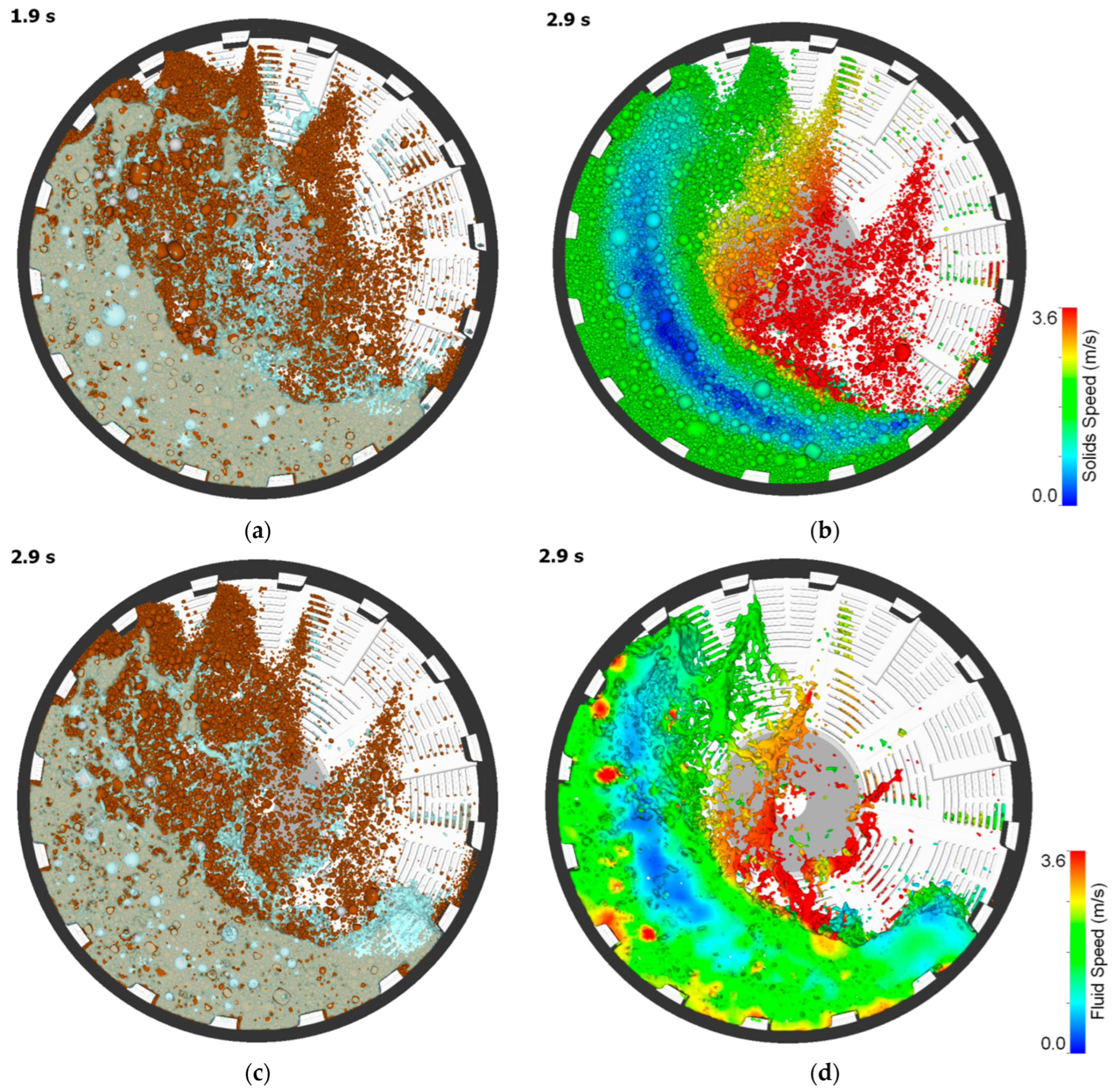
Figure 3 shows the flow in the Hardinge pilot mill viewed in the axial direction looking towards the discharge grate (with the feed half of the mill removed to provide visibility of the internal flow structure). The visualisation is created from the DEM and SPH simulation data using an in-house Workspace based flow visualiser with supporting workflows [34]. Figure 3a,c show the rocks and media as brown and the slurry as light blue at two times. The charge structure has its usual SAG mill form with particles distributed between the toe and shoulder, with a coherent cascading flow from the shoulder to toe and a substantial cataracting stream. The slurry fills the void space in the solid charge and occupies a similar region but there is some difference. The slurry shoulder is lower than the solid shoulder, and a small slurry pool is located above the solid toe. The slurry structure within the cataracting part of the flow is quite variable, reflecting the specific details of draining from the regions between the lifters, which depends on the solid particle distributions between each pair of lifters. Some material within the pulp chamber can be seen through the discharge grate. Figure 3b shows just the solid phase (coarse resolved DEM particles) coloured by their speed. This shows the usual and expected speed distribution with material near the liner moving near the speed of the liner with decreasing speed away from it. The curved band of low-speed material (dark blue) separates the upward-moving material below this from the downward-moving material that is above. The cataracting stream has the highest speeds with many direct impacts between the impact toe and bulk toe of the charge. Figure 3d shows the slurry phase only, coloured by its speed. This has a generally similar distribution with some finer scale variation, which results from the need for the fluid to flow within the solid charge as it deforms and shears, forcing the fluid around larger particles.

Figure 4 shows the flow of slurry in and from the Hardinge mill, as seen from the front with the mill section that was removed to enable visibility of the sub-surface flow structure coloured by fluid. In Figure 4a, the slurry is coloured by its speed, which is similar and moderate (green) in many locations. The flow of the new slurry along the feed chute into the mill is clearly visible. Flow through the grate and into the pulp chamber (bottom right) is also clearly observable. The pulp chamber in this case is around 25% filled. Flow from the pulp chambers that are near the top of the mill onto and along the discharge cone and out of the mill is also clearly shown. The fluid surface level is strongly elevated at each end of the mill, reflecting the strong lifting effect of the end wall lifters. The cataracting slurry is fragmented and appears in the form of ribbons or sprays of slurry from the belly and end wall lifters. This slurry is coloured red as it is the highest-speed fluid in the mill. Figure 4b shows the same slurry coloured by its axial speed. This colouring clearly shows the effect of the entry of the feed slurry stream into the charge with momentum from the feed stream continuing to push the slurry to the right (red). To the left of the impact location, the slurry (dark blue) is forced back towards the feed end of the mill. The large fairly coherent concentrations of red and dark blue in the sectioned area of the toe show that the slurry has strong turbulent behaviour, which is driven by the regular impact of the end wall lifters driving into the charge and generating significant sloshing and splashing behaviour in the part of the charge near the toe. The axial colouring also clearly highlights the discharge flow from the elevated pulp chambers along the discharge cone. The flow from the top of the discharge end is stronger, and the slurry starts higher up than on the feed end as a result of significant backflow from the elevated pulp compartments back into the grinding chamber.

Figure 3 and Figure 4 show that slurry action within the pilot mill at a steady state is quite vigorous, suggesting that mixing is likely to be reasonably effective. However, considering dynamic mixing as the mill starts up, the evolution of this fully developed slurry flow state of strong mixing is gradual and requires several revolutions of the mill.

Figure 5 shows the progress of axial transport and mixing of the new slurry (red) being added to the mill into the multiphase resident charge (light blue). Figure 5a shows the initial contact of the feed stream with the charge. The stream from the chute is pushed downward before it reaches the slurry surface by the large cataracting stream. One second later (Figure 5b), the new slurry has been distributed along the bottom of the mill and to some of the outer layers of the charge. By 2.4 s (Figure 5c), the new slurry is transported around the mill and has reached perhaps 2/3’s of the mill charges. This continues with a new slurry part filling the shoulder region of the charge by 2.9 s (Figure 5d). Further feeding of the slurry leads to general flow in the axial direction and increasing concentration in the feed half of the mill. The new slurry starts to pass through the grate (bottom right of Figure 5e) at 3.9 s. This indicates an approximate residence time of 3 s for the slurry in the Hardinge mill. By 4.9 s, the new slurry (red) can be seen in the flow on the discharge cone, and the new slurry starts to exit the mill.

The glyph-based rendering used for the new slurry (shown in red in Figure 5) makes depth interpretation difficult. One might be tempted to conclude that the slurry phase of the mill charge is well-mixed in any axial slice. However, Figure 6 (which shows an axial slice of the slurry phase at two times with the same style of rendering as Figure 5) clearly shows that the new slurry is strongly concentrated around the outside of the mill and at later times is heavily concentrated in the toe region. When the new slurry enters, it arrives on the free surface a little to the right of the centre of the mill due to momentum gained from interaction with the cataracting stream. This slurry spreads over the nearby surfaces. A concentration of red can be seen in this region in Figure 6a. The strong circumferential circulation that occurs in a tumbling mill charge then transports this slurry to the toe where it is subducted down under the charge and is trapped by the solid charge near the liner. It is then drawn up by the usual upward shearing flow of the charge towards the shoulder, which creates the distribution observed in Figure 6a. As more slurry is added, the pattern of distribution continues, leading to greater concentrations in these regions. It is highly instructive to observe that there is very little slurry entering the bulk of the circulating charge. This highlights one of the key sources of the inefficiency of an SAG mill, the strong difficulty in getting the new slurry into most of the charge and getting the ground slurry back out. This means that a spatially large fraction of the SAG charge is limited in the contribution that it can make to slurry phase grinding, as it contributes to the over-grinding of the slurry in these regions. Fortunately, the area under the toe where slurry access is quick and efficient is also the region where the DEM predicts that high rates of energy dissipation occur. In these regions, the new slurry can enter, and the ground slurry can be removed. But more than half of the SAG charge is limited in the contribution that it can make to finer grinding. In the Hardinge mill, as shown in Figure 3d, the slurry component is vigorously mixed at a steady state even though it takes a revolution or two to reach that state.

Next, we consider the flow in the pulp chamber. With this two-way coupled DEM + SPH model, the discharge of both coarser particles “pebbles” and the slurry can be predicted. Figure 7 shows the fully developed flow, with all the pulp chambers having been filled and at least partially discharged. The slurry fill levels (light blue liquid in Figure 7a,b) are substantial in the chambers in the bottom right quadrant. The slurry enters the pulp chamber in the lower sections from the toe back to the middle of the mill. Very little flow is observed through the high slots (nearer the centre of the mill), with the dominant contributions arising from slots nearer the mill shell since these slots have much higher hydraulic pressures driving the flow. Significant volumes of pebbles (brown rendered particles) have also entered the pulp chamber and have built up against the liner at the bottom.

As the pulp chamber rotates, the pulp compartments re-orient, causing the slurry and pebbles to flow. The pebbles settle towards the outside bottom corner of each compartment. The slurry flows radially inward as the pulp lifter underneath rises towards the 3 o’clock location. Above this radial flow towards the discharge, the cone accelerates and a significant amount of slurry discharges from the mill. The pebbles, however, are still in the outer corner, even as the pulp lifter reaches the 1 o’clock position. Pebble flow becomes faster and more substantial after the pulp lifter passes vertically, but this is too late for the pebbles to reach the discharge cone, and a significant fraction falls onto the back of the preceding pulp lifter and is recycled. Some slurry is trapped in its original pulp compartment, while some is deflected from the discharge cone back into the previous pulp compartment where it is also trapped and recycled.

Figure 8 shows the measured quantitative flow rates through one grate panel over the first three revolutions of the mill. The solid line shows the flow rate of particulate solids (coarser sub-grate scale particles or “pebbles”), while the dashed line shows the slurry flow rate. This slurry flow rate strongly peaks at the start of the flow through the panel, reflecting the slurry having its highest mobility near the toe before the solid charge settles and becomes more compact, restricting slurry flow later on. Also, as the pulp chamber fills, it becomes harder for additional slurry to enter. The details of the slurry discharge rate vary between revolutions, but the general features of discharge are similar. Note that the peak slurry rate declines between revolutions, which reflects the partial draining of the discharge end of the mill, as axial slurry transport within the grinding chamber becomes limiting and the decreasing slurry available at the discharge end reduces the grate flow rate. The pebble discharge into the pulp chamber starts much later than the slurry flow.

The average slurry discharge rate over the first three revolutions is around 5.0 kg/s. Since there are eight pulp chambers, the early overall slurry grate discharge rate is about 40.0 kg/s. This is much higher than the slurry feed rate of 6.0 kg/s and indicates that the Hardinge pilot mill is very effective at pumping slurry from the mill. This suggests that the initial slurry fill level is higher than the steady-state slurry load in the charge. The average pebble discharge rate is 0.18 kg/s through the selected grate, so the overall grate discharge rate for the eight pulp chambers will be around 1.4 kg/s. This is actually relatively close to the rock feed rate of 1.11 kg/s. Exact matching of the rock feed and discharge rates cannot be expected with this generation of model, as the coarse breakage of rock is not enabled, and the rock component of the slurry has also not been included in the discharge flow rate.

Figure 7c,d show the slurry phase only but this time coloured by the concentrations (solid fractions) of slurry size fractions 6 and 8 (third finest and finest slurry size fractions). Recall that the particle scale model uses the information on the local energy dissipation rate from the DEM sub-model to inform a local PBM model for the slurry phase grinding (size reduction) of these fine slurry fractions. This means that with the inclusion of the slurry feed and the flow through the grates, the model can directly predict (although currently with unknown accuracy) the rate of discharge of each product size fraction, as well as their spatial distributions within the pulp chamber. These are clearly not well-mixed and have quite strong spatial variations within each pulp compartment depending on whether the slurry entered through the leading or trailing sub-panel. The sub-panel pair is divided by the discharge end lifter (which is in the middle of each pulp compartment) that agitates the charge adjacent to the grate and generates a strong pumping action that causes different slurry streams to enter the pulp chamber through the leading and trailing regions.

Figure 9 shows the flow on and from the discharge cone fed by flow from the pulp chambers and the grate behind. Figure 9a shows the complete multiphase flow, with coarse rocks in brown and the slurry coloured light blue, while Figure 9b shows the concentration of the finest slurry size, fraction 8.

The steady-state net power draw predicted for the Hardinge with non-spherical rocks, round balls, and the slurry is 8.57 kW [31]. This compares to 8.89 kW predicted by pure DEM for a dry version of the mill, which represents a 1.8% reduction. This power cannot be meaningfully compared to published power models because the configuration of the 36 ft mill used here, having been scaled up from the Hardinge pilot mill, is sufficiently different from most industrial mill designs, particularly in terms of the lower number of belly lifters.

Power comparisons with actual pilot mills are complicated by the much higher proportion of no-load power compared with an industrial-scale mill. However, a comparison with a small pilot mill with power draw well-measured by a torque balance produced an excellent agreement between the measured and the DEM predicted for two different DEM systems [16]. It is worth noting that the Hardinge simulation exhibits a slurry pool, which is expected to reduce the power drawn.

Of the power input, 19.5% is contributed by the discharge end lifters and grate structure, which provides significant lift to the charge that is proportionally larger than the belly lifters. Since the feed end lifters are similar to those of the discharge end, assuming a similar contribution from the feed end wall means that the belly lifters contribute only around 60% of the power supplied to the charge, with each end wall providing a significant 20% of the power draw.

The inter-particle energy dissipation, however (from the DEM part of the model), is only 7.77 kW. The remaining energy dissipation can be attributed to the dissipation in the slurry (arising from viscous forces). This means that around 9% of the power draw is dissipated in the slurry phase. It is not clear that any of this energy dissipation will lead to useful comminution of the fine particles within the slurry. This means that the inclusion of the slurry has reduced the energy dissipation in the solid particle phase, which should not be entirely unexpected.

Figure 10 shows the collision energy spectra for the solid charge. This shows the normal and shear components and the distribution of the total energy per collision. The spectra have a conventional shape that is approximately a normal distribution with a clearly defined modal peak. They can be used to characterise the collision intensity (which controls the breakage). The collision spectrum for this wet Hardinge mill is structurally similar to the dry mill [31]. The location of this modal peak was at 2.2 mJ for the dry mill. For the wet mill, this has increased to 3.7 mJ. The detailed micromechanical origins of this increase are not yet understood. The corresponding peak energy dissipation rate is close to 40 W for both wet and dry versions of the mill. The rock–rock collisions consume 82% of the energy dissipated by the charge (recalling that this is 91% of the power draw). Rock–liner collisions dissipate 7%, while rock–media consume 10%. Media–media collisions consume only 0.5% of the energy because the ball load at 5% is relatively low, resulting in low frequencies of media–media collisions.

4. Multiphase Flow into, within, and from a 36 ft Industrial Mill

Next, we consider the solids and slurry flow inside and discharge characteristics from an industrial scale 36 ft SAG mill that is a scaled-up version of the Hardinge mill. The diameter scaling is by a factor of 5.93×. A traditional power scaling approach would use the product of the grinding length ratio and the diameter ratio raised to the power of 2.5 or 261 times at similar mill operating conditions.

A pure scale-up is not sufficiently consistent with real mills, so some necessary adaptations are required in the grinding chamber, but we have attempted to retain as many of the features from the pilot mill as possible. This is intentional so that we can directly explore the relative mill performance and slurry flow for the two mill scales.

The mill geometry is shown in Figure 11. The geometric dimensions (and rotation speed) of the 36 ft mill are given in

Table 4. Dimensions and key geometric parameters for the 36 ft SAG mill.

36 ft Scaled up SAG Mill	Dimensions
Mill diameter (internal)	10.4 m
Rotation speed	79% critical (10.4 rpm)
Rotation of mill	clockwise
Grinding chamber axial length	4.8 m
Pulp chamber axial length	534 mm
No. of belly lifters	48
Belly liner plate thickness	268 mm
Belly lifter height	170 mm
Belly lifter base width	211 mm
Belly lifter face angle	73.3 degrees
Feed end wall—conical angle	74.8 degrees
No. of feed end lifters	24
Feed end lifter height	259 mm
Feed end lifter base width	270 mm
Feed end lifter face angle	90 degrees
Discharge end wall—conical angle	79.1 degrees
No. of discharge end lifters	8
Discharge end lifter height	275 mm
Discharge end lifter base width	384 mm
Discharge end lifter face angle	90 degrees
Grate slot width (outer radial)	90 mm
Grate slot width (inner radial)	60 mm
Grate axial thickness	153 mm
No. of pulp lifters	8
Pulp lifter height	479 mm
Pulp lifter base width	630 mm
Pulp face angle	90 degrees
Diameter of trunnion opening	3.24 m
Length of trunnion	1.485 m

. The mill shell is supported by feed and discharge trunnions. In the grinding chamber, there are radial feed end wall lifters at each end and belly lifters around the circumference. The belly lifters have a simple trapezoidal shape. There is a moderate complexity grate separating the two chambers. The grate structure in particular is a direct scale-up of the Hardinge grate, so there are two sub-panels between each pair of discharge end lifters. The pulp chamber contains eight radial pulp lifters, which act to transport the slurry out to the discharge trunnion via the discharge cone, after which it exits the mill.

Features that were varied in the grinding chamber from a pure scale-up of the Hardinge mill were made to account for more recent industrial design practices. A pure geometric scale-up of the belly lifters does not make dynamical sense. The internal belly length was, therefore, increased to give a mill aspect ratio of 36 ft × 16 ft (EGL), which matches a 12,680 kW Metso mill [41]. A direct geometric scale-up would have a length of 12 ft. Belly lifters cannot be directly scaled up, so we have used 48 rows of moderate-size lifters. In contrast, the pilot mill has 16 rows of relatively larger lifters. Note that the end wall lifters have been retained at their pure scale-up dimensions in order to understand their impact on axial slurry flow, even though they are very physically large and aggressive in terms of the lift and throw that these end walls then generate. More traditional industrial mill liner configurations would have 72 rows of lifters but in practice can include reduced numbers of rows, so we have accordingly used 48 rows. Also note that the grates are directly scaled up and are quite large compared to the rock and ball particles for which broadly similar distributions are used. This is a consequence of the general practice of using the same feed size distribution in the pilot and the full-size mill. This means that the coarse particles are relatively much larger in the pilot mill. Since the charge size distribution is not scaled up, at the full scale, the grates are relatively much larger than they are at the pilot scale. In typical full-size mills, the grate slots would be narrowed from the scaled-up sizes. But since the intent of this paper is to look at the relative performance of the two scales, we use the scaled-up grate size. The scaling up of the Hardinge design to 36 ft introduces many other secondary issues, where scaled-up values differ from current industrial practice. One such example is the thickness of the belly liner plate, which, when scaled up, is 268 mm and is larger than would be used in practice. Since the liner plate thickness mostly affects the mechanical behaviour of the mill and the wear life, which are not considered, we note such differences without seeking to change them.

The fill level of the charge in the full-size mill is reduced to be closer to more modern practice. Modern operations would not usually use a fill level as high as 39% and, with the large scaled-up slots, such a fill level would lead to a total overload of the pulp chamber, so a lower fill level of 25% (by volume) with 8% media is used. The size distributions (PSDs) for both media and rocks are given in

Table 5. Particle size distributions (media and rocks) used in the 36 ft SAG mill.

Ball Class	Size Fraction (mm)	Percentage of Ball Load (%)
B1	75.0–105.0	30
B2	52.0–75.0	30
B3	37.0–52.0	30
B4	25.0–37.0	5
B5	15.0–25.0	5
Rock Class	Size Fraction (mm)	Percentage of Rock Load (%)
R1	102.0–122.0	0.65
R2	76.0–102.0	1.74
R3	53.0–76.0	6.01
R4	40.0–53.0	12.24
R5	30.0–40.0	22.13
R6	24.5–30.0	57.23

, with the minimum resolved DEM particle size scaled up to 24.5 mm. Material that is smaller than this but larger than the 6.5 mm top size for the slurry phase is added to the last resolved size fraction (24.5–30 mm). The media density is 7850 kg/m³ and the rocks are 2900 kg/m³. Again, the resolved particulates are represented by super-quadric shapes, with the media essentially spherical and the rocks varying in shape from near-round (m = 2.5) to blocky (m = 4) with modest aspect ratios. The particle shapes used are the same as the pilot mill. The slurry feed rate is 3100 m³/h. Rock feed was omitted in this case because the simulation was not sufficiently long for rock feed to materially change the charge mass. Also note that in the absence of coarse rock breakage, including rock feed is not meaningful.

Figure 12 shows the flow in the 36 ft SAG mill viewed in the axial direction looking towards the discharge grate with the feed half of the mill removed to provide visibility of the internal flow structure. Figure 12a shows the rock in brown, the media in grey, and the slurry in light blue. The charge again has a customary SAG-type distribution. The slurry is concentrated from the toe region around to just under the shoulder. With the lower fill level and relatively smaller belly lifter used for the 36 ft mill, there is little slurry entering the strong cataracting solid flow. At this scale, the individual DEM particles are very difficult to resolve, and the solids look almost like a continuum, but the solid phase is both modelled and rendered as particulates. Figure 12b shows the coarse resolved particles (DEM) coloured by their speed. The velocity distribution is again consistent with many previous dry DEM simulation results, as the bulk of the solid charge is not strongly affected by the presence of the slurry. Figure 12c shows the slurry phase coloured by its speed. This closely reflects the DEM (solids) velocity distribution, which is a well-established consequence of the dominance of the solid phase in this part of the mill. The slurry within the pulp chamber can be seen through the grates. The structure of the relatively low trajectory slurry cataracting stream (that was hidden by the solid component in Figure 12a) can clearly be seen above the main slurry-free surface (in Figure 12c).

Figure 13 shows the flow of the solids and the slurry coloured by their respective axial speeds. Near the centre of the mill, there is little axial flow, so both are coloured green. In the feed half of the mill, there is a very strong flow away from the end walls from the shoulder position and above. This axial flow away from the end wall is very strong because of the large size of the scaled-up end wall lifters. There is a counter-balancing strong axial flow back towards the end wall as the toe is approached. Similarly, at the feed end, there is a strong flow away from the discharge end walls as the end wall lifters lift large volumes of solid charge, which then fall away towards the centre of the mills as these lifters rise. Again, there is a strong counter-balancing flow back towards the discharge end in the region approaching the toe.

The flow is strongly enhanced by the flow of the solid charge through the grate and into the pulp chamber. The slurry flow pattern is very similar in many regions. The stream of the new slurry arriving from the feed chute is coloured red and generates the same types of flow in the upper section of the slurry as it did for the Hardinge pilot mill. There is strong axial flow away from the end walls, corresponding to the solid flow in these areas. This manifests in both the solid and slurry flow as two large axial circulation eddies. This means that the mill cannot be assumed to be well-mixed. The slurry flow in the bottom right accelerates very strongly through the grate and into the pulp chamber. For the Hardinge mill, we observed some backflow from the elevated pulp compartments back into the grinding chamber. Looking carefully at the top right of Figure 13b, it is clear that the extent and strength of the backflow is much larger for the 36 ft mill. This clearly demonstrates that the transport behaviour changes very strongly with the physical scale of the mill, even though the pulp chamber and grate have the same structure (differing only by a direct scale-up from the Hardinge).

Figure 14 shows the progress of the transport and mixing of the new slurry (red) added to the 36 ft SAG mill from two views where the multiphase resident slurry is coloured light blue. The new fluid is pulled around the feed end wall by the radial lifters so that there is greater new fluid volume at the feed end (clear axial distribution of red slurry volume). The slurry circulates faster in the circumferential direction (being dragged around by the surface of the charge and the action of the lifters) than the axial transport. The radial transport into the core of the charge is very slow. In the front-on view, the new slurry looks well-mixed, but this view is deceiving with the axial view, showing that the new slurry is concentrated around the very outside of the charge. By 6.5 s, the Hardinge was becoming well-mixed, and significant amounts of new slurry were already exiting the mill. For the 36 ft mill, the rate of axial transport is much slower (so that the amount in the centre plane is significantly less than the Hardinge, as shown in Figure 6). So, the mixing is poor, and the axial transport is much slower. This is a consequence of the larger physical scale and the relatively longer belly length and clearly demonstrates that slurry transport does not scale up well with increasing mill size (which is anecdotally well-known and attributed to a decrease in the surface-to-volume ratio with increasing mill size). It should also be noted that the behaviour demonstrated contains very large end wall lifters. If more usual end wall lifters were used, one would expect further reductions in mixing and transport rates.

Figure 15 shows the flow through the grate within the pulp chamber of the 36 ft SAG mill. Figure 15a shows a multiphase representation with the rock coloured brown and the slurry coloured translucent light blue. The simulation has run sufficiently to fully load all the pulp compartments, which then show the flow at a range of the angles of the pulp lifters and different levels of both solid and slurry fill. The earliest-to-fill compartments have very high solid loads since there is a surge of solid discharge driven by the establishment of the flow pattern within the grinding chamber and because there are significant amounts of sub-grate scale particles adjacent to the grate at the start. The lower pulp compartments have smaller volumes of solids, and the flow of solids into the lower compartments through the grate slots can be clearly seen. It should be noted that the slurry volumes are relatively lower for the 36 ft mill compared to the Hardinge, which reflects both the lower charge fill level and the intrinsically greater difficulty of discharge for the larger mill. In contrast, the number of solids is relatively much larger for the 36 ft mill compared to the Hardinge, which is predominantly the result of the large scaled-up grate slot dimensions. It is very interesting to observe that the solid discharge behaviour and the slurry discharge behaviour scale differently with mill size. This represents yet another challenge in designing optimal mills at each size. Figure 15b shows the slurry phase only coloured by the solid fraction of the second finest slurry size fraction. Again, large spatial variation is observed both within and between pulp compartments. This also demonstrates that this type of particle model can, in principle, directly predict the product size of the mill.

The simulation duration was 26 s (around four revolutions of the mill). The slurry discharge rate from the mill (exiting through the discharge trunnion) becomes steady at about 12 s. The average slurry discharge rate is then 0.58 m³/s. The slurry feed rate used in this simulation was 0.87 m³/s, so the slurry fill level rises slowly but steadily throughout the simulation. The slurry discharge rate from the mill is, however, constant, so this means that the mill is at its pumping capacity limit (for this mill speed and charge fill level), which is 0.58 m³/s. Steady-state operation then requires a slurry feed rate that is lower.

In contrast, the pebble discharge rate is very low until about 14 s and then increases steadily to around 120 kg/s at 26 s, which is equivalent to 400 tph of resolved particle product. Discharge is hampered by particles falling into the trunnion and requires a build of particles in order to generate axial flow along the trunnion and out of the mill. This highlights the reason for typically including at least one spiral baffle in the trunnion to force a steady discharge of pebbles that are delivered to this region by the flow from the discharge cone.

Figure 16 shows the measured flow rates from the simulation through one grate panel over the first four revolutions of the 36 ft SAG mill. Slurry flow occurs periodically as the middle and end of the grate panel are submerged below the level of the charge in the grinding chamber. The slurry flow rate increases progressively, with each revolution reflecting the increase in the slurry fill level and the internal rearrangement of the solid charge in the grinding chamber near the grate (specifically the effect of the cumulative discharge of finer material from the charge in the vicinity of the grate, which increases the permeability of the charge and therefore the slurry mobility). There is a secondary structure in the flow rate during peak flow, which varies between revolutions and to which we currently do not attach dynamical significance.

It is useful to compare the relative slurry flow rates into the pulp chamber for the two mill sizes. The average discharge flow rate through the grate in the pilot mill is around 5 kg/s (Figure 8). Since the spatial scale-up is by a factor of 5.93, volumes scale by a ratio of 208. On this basis, one might expect an average slurry discharge flow rate for the 36 ft mill in the order of 1040 kg/s. The average flow rate through one grate panel of the simulated 36 ft mill is only around 300 kg/s, which is about a third of the theoretical scale-up capacity. This demonstrates the known decrease in pumping and discharge capacity as mills increase in physical size and allows an estimation of the reduction in transport efficiency of a geometrically equivalent scaled-up grate of about 65%.

The overall average slurry discharge rate for all the grates is calculated to be around 2400 kg/s (300 kg/s for each grate by eight grates). This is also much larger than the slurry feed rate of 1000 kg/s, meaning that the scaled-up 36 ft also initially has too high of a slurry fill level. The excess pumping capacity of the pulp chamber compared to the slurry feed rate for the 36 ft mill is a ratio of 2.4, which is much lower than the 6.7 ratio found for the pilot scale mill. So, although the scaled-up mill is able to still pump quite a lot of slurry and reduce the slurry fill level over time, it is much less effective than the pilot scale mill. It also means that the equilibrium slurry hold-up in the mill will be meaningfully higher for the 36 ft mill than the pilot mill. This demonstrates that the scale-up behaviour of slurry transport is not good for SAG mills.

The under-design of pulp lifters for full-scale mills is not uncommon. Morrell and Latchireddi [42] reported an industrial installation that had an insufficient pulp lifting capacity. Fitted with a novel pulp lifter design, mill capacity increased from 390 tph to 450 tph at a similar pulp load. Powell and Valery [43] investigated a wide range of SAG mills with different diameters and concluded that a better understanding of pulp discharge was required, especially for large-diameter mills in closed circuit with cyclones.

The pebble flow rate (Figure 16 solid line) is very high at the first exposure of the grate panel to the charge, with the finer charge material in the grinding chamber surging into the initially empty pulp chamber. After this initial peak, the pebble flow rate decreases steadily, as it is increasingly limited by the slower axial flow of replacement finer rocks from the axial middle region of the charge towards the grate. So, the internal transport of the finer rock in the grinding chamber can be identified as a key limit on the pebble discharge rate through the grate.

In the latter half of the period over which a grate panel is submerged below the charge-free surface, the pebble flow rate is observed to be strongly negative. This indicates that pebbles are flowing back from the pulp chamber into the grinding chamber during this phase. In contrast, the net slurry flow remains positive (Figure 16, dashed line), which means that the slurry continues to flow into the pulp chamber throughout its rotation through the charge. The explanation for the pebble behaviour is, therefore, not the commonly observed backflow that can occur as the pulp lifter becomes elevated and the residual slurry drains back into the grinding chamber (see [12]). In the current situation, the slurry is, on average, flowing into the pulp chamber, while the pebbles are flowing back out. The slurry in the vicinity of the pebbles must necessarily also be flowing back out. What is shown in Figure 16 is the net flow rate, which in this case is a combination of strong flow into the pulp chamber that is partially balanced by backflow elsewhere. Since the pebbles settle quickly towards the shell and the pulp lifter, we hypothesise that the slurry flow into the pulp chamber occurs closer to the mill axis (which corresponds to the region with the cascading surface of the charge, which allows reasonable slurry mobility, enabling flow into the pulp chamber). Within the pulp chamber, the increasing depth of the slurry exerts significant hydraulic pressure that forces fluid and particles near the bottom of the mill back through the grate into the grinding chamber (via the slots near the mill shell). This region is pebble-rich, so there is entrainment of a significant number of these pebbles, causing strong pebble flow back through the grate into the grinding chamber. This behaviour is not observed in the much smaller Hardinge pilot mill. Its pebble discharge rate is small and remains positive over time (Figure 8). This reflects the relatively larger size of the pebbles compared to the grate slot width and the much lower hydraulic pressures generated over the smaller height of the pilot mill. This indicates that pebble removal becomes more difficult with increasing mill size and is likely to require some form of design alteration to counteract at least some of this scale-up-related reduction in pebble discharge rate.

The peak pebble discharge rate in the 36 ft mill is significantly stronger than the Hardinge mill because the slots are relatively larger compared to the average and minimum resolved coarse particle size. In the Hardinge mill, the slurry flow rate into the pulp chamber in the second half of the filling phase is relatively much weaker (again reflecting the restrictive effect of its relatively narrower slots). This also means that there is not a very strong slurry flow through the inner sections of the grate into the pulp chamber. This combined with the much smaller physical scale of the mill means that the hydraulic pressure head from the top of the slurry pool in a pulp chamber to its bottom is much smaller (than the 36 ft mill) and is not sufficient to generate a strong basal flow from the lower parts of the pulp chamber back into the grinding chamber. The pebble flow rates indicate that there is no pebble backflow into the grinding chamber. There is, however, some slurry backflow visible in the visualisations when the loaded pulp chamber rises above the charge shoulder, but this remains smaller than the positive flow into the pulp chamber from the still submerged slots, which leads to a net positive flow rate into the pulp chamber throughout the pulp chamber filling cycle.

The steady-state net power draw predicted for this 36 ft SAG mill is 6.50 MW, which is a sensible level for such a mill with such a low number of belly lifters operating at this speed and type of charge. As the simulated mill has many fewer lifters than a typical industrial mill of this size—around 72—the scaled-up mill will not lift as many liner loads per unit of time and will draw less power than a semi-empirical model would predict based on a calibration with standard industrial practice.

Regarding power input, 12.6% is contributed by the discharge end lifters and grate structure. This is quite large but meaningfully smaller than the 20% found for the Hardinge pilot mill from which this 36 ft mill is broadly scaled. Assuming a similar level of contribution from the feed end, this means that the belly lifters contribute around 75% of the power supplied to the charge, with each end wall providing around 12.5% of the power draw. The reduced relative contribution of the end walls can be substantially attributed to the lower aspect ratio (greater length of this mill). Scaling the Hardinge mill length (0.509 m × 5.93 m) gives a scaled-up equivalent length of 3.02 m. The grinding chamber length used is 4.8 m, which is approximately 1.6 longer than a direct scale-up. A simple scale-up calculation where the 60% contribution of the belly lifters is increased by the proportional grinding chamber length and the power is re-normalised gives an estimate of 29% for the end walls and 71% for the belly lifters, which is very close to the simulation prediction. This demonstrates that the contribution of the belly lifters to the power draw and, therefore, the overall dynamics is basically proportional to the length of the grinding chamber and supports the relationship used for traditional power-based scale-up [44].

The inter-particle energy dissipation, however (from the DEM part of the model), is only 5.5 MWW. The remaining energy dissipation is again attributed to the dissipation in the slurry phases from the viscous interactions. This means that around 15% of the power draw is dissipated in the slurry phase in the 36 ft mill. This is meaningfully larger than the Hardinge mill (which was only 9%). So, at an industrial scale, 1 MW (or 15% of the power draw) is most likely dissipated without obviously contributing to the comminution because of the presence of the slurry phase. This is the price that needs to be paid by the process in order to gain acceptable fine particle transport in the system.

Figure 17 shows the collision energy spectrum for the solid charge for the 36 ft SAG mill. This shows the distribution of the normal and shear components and the total energy per collision. The spectrum strongly peaked at a collision energy of 170 mJ with a corresponding energy dissipation rate of 50 kW for that spectrum bin. In contrast, the modal peak collision energy for the Hardinge pilot SAG mill (Figure 10) is 3.7 mJ. This means that the average collisions experienced by rocks in the 36 ft mill are around 46× stronger than the Hardinge pilot mill. The spectrum for the large mill is also significantly more sharply peaked and more skewed to the right than was found for the Hardinge mill (Figure 10). The normal distribution is also quite different with a secondary peak at higher energy and a very different distribution shape compared to the shear energy distribution. The high energy part of the spectrum also drops off much more sharply, which means that there are relatively fewer very strong collisions. This is a consequence of the larger number of rows of proportionally smaller belly lifters (in the 36 ft mill), which means that the large mill has a relatively weaker cataracting stream, which reduces the amount of very high energy impacts that is available for breakage. This contributes strongly to the skewness of the collision energy distribution. The lack of similarity in the nature and intensity of the collisions that are generated by these mills calls into question the value of using such a pilot (or smaller mills) for ore characterisation and estimation of the comminution performance of large mills. The micro-mechanical behaviours exhibited at the particle scale, which drive fundamental breakage, are sufficiently different so as to make the extrapolation of dynamical behaviour problematic between such scales.

Perhaps one saving grace in terms of the ability to scale up such a mill is that large rocks in both the 6 ft and 36 ft mills are predominantly reduced in size by attrition, which depends largely on the power intensity within the charge. However, it is also worth remembering that when scaling up from pilot testing dominated SAG design, a “large” SAG mill might be 24 to 28 ft in diameter. This is a significantly less demanding degree of scale-up. Very large SAG mills, say 40 ft and larger, require a relatively small database of published data for pilot and full-scale operation. The designers of the first 40 ft SAG mill installation [2] used traditional methods and all of the simulation methods available at the time to reduce the risk of a large increase in mill capacity as much as they could. If the DEM combined with SPH had been available at that time, it seems likely that the designer team would have used it as well.

The rock–rock collisions consume 61% of the energy dissipated by the solid charge (which is meaningfully lower than the 82% found for the Hardinge mill). Rock–liner collisions dissipate 2.4% (down from 7% for the Hardinge), while rock–media consume 32% (which is sharply increased from 10% for the Hardinge model). Media–media collisions consume 4% (sharply increased from a small base of 0.5% for the Hardinge). So, the distribution of energy consumption between the different types of collisions is quite different for the two models. The attribution of these differences to changes in the dynamical behaviour between scales is complicated by numerical issues relating to the effect of the size cut-off for the rocks, which controls which particles are explicitly resolved in the DEM component of this model. For the Hardinge model, particles down to 6.5 mm are resolved, which means that there are almost always rock particles between all other colliding entities (hence the very low fraction of media–media collisions). In contrast, the resolved size limit for the 36 ft SAG model is 24.5 mm, which is much coarser and means that many more direct media–media collisions can occur because of the much smaller range of fine particles that are available to separate them (causing much of the eight-fold increase observed here). The minimum resolved size was decided on the basis of the minimum rock size that makes sense for inclusion based on the grate slot size, which controls the discharge and, therefore, the lower end of the resident rock size distribution present. So, to some extent, the increase in media–media collision rates is a real reflection of the reduced fractions of finer particles due to discharge behaviour, but there is also likely to be a contribution from the computational approximation of the charge. At the moment, these two effects are both poorly understood and cannot be fully separated. In the interim, some caution needs to be used when considering the specific quantum of the changes observed.

5. Discussion

The principal observations from the pilot scale model include:

• The presence of the slurry does not appreciably change the flow behaviour of the coarse particle fractions of the charge in the grinding chamber, which behaves in much the same way as predicted for a dry system by the DEM alone.
• The slurry motion within the grinding chamber has significant sloshing in the slurry pool as the cascading flow plunges into the pool. There is strong three-dimensional axial recirculation of both solids and slurry, with strong flow away from the mill ends in the upper parts of the charge and strong flow back towards the end walls in the lower parts of the charge.
• Feed slurry is not able to mix effectively with the resident charge, and much of the feed slurry bypasses the grinding parts of the charge by flowing through the slurry pool and quickly exiting the mill. Slurry already in the high shear/high dissipation regions of the solid charge demonstrates poor mobility, which will lead to it being over-ground.
• The model is able to predict significant rates of both slurry and pebble flow into the pulp chamber.
• The pilot scale mill is very effective at pumping slurry from the grinding chamber of the mill, and high-volume fill levels can be found in the pulp chambers.
• Slurry flow down along the pulp lifters tends to initiate at around the 2 o’clock position. In contrast, the pebbles that have settled to the bottom of the pulp chamber do not initiate downward flow until they are vertical. Significant amounts of slurry and pebble carry-over are observed, with complex high-volume flow occurring into previously partially emptied pulp chambers.
• Slurry size fractions (which are ground in the grinding chamber) are not well-mixed upon entry into the pulp chamber. There are quite strong spatial variations within each pulp compartment depending on whether the slurry entered through the leading or trailing sub-panel. This means that there will be strong short-term fluctuations in the discharging product size distribution.
• Discharge from the pilot scale mill via the discharge cone is significantly less effective than discharge from the grinding chamber into the pulp chamber.
• About 9% of the power draw in the pilot mill is dissipated in the slurry phase for the solid loading (and, therefore, viscosity) considered here.

The 36 ft SAG mill used for the scale-up comparison was constructed to be as close to a geometric scale-up of the Hardinge as possible. However, some design features required modification. These include the mill aspect ratio, which was chosen to correspond to a popular 36 ft × 16 ft design. Belly lifters also cannot be directly scaled up; otherwise, they would be unphysically massive, so 48 rows of moderate-size lifters were used instead. The end wall lifter structure was retained so as to understand its impact on axial slurry flow. Similarly, the grate and pulp chamber were directly scaled up from the pilot mill. This geometry retains as many of the features from the pilot mill as possible. This is intentional so that we can directly explore the relative mill performance and slurry flow for the two mill scales. Scale-up from the Hardinge 6 ft × 2 ft pilot mill to an industrial scale 36 ft mill; that is, from 9 kW to 6 MW, which is a factor of more than 650 times, represents a major theoretical challenge.

Comparison of the performance of this 36 ft SAG mill with the 6 ft pilot mill provides important insights into the scale-up challenges for SAG mill design. It shows:

• The collision environment is very different between the two mills, with the larger mill having much stronger collisions. This will give very different body breakage behaviour that appears to be barely correlated between the two scales.
• Slurry transport within the grinding chamber is slower, and the mixing of slurry into and out of the solid charge (where grinding occurs) deteriorates. Axial flow is much slower, and radial transport into and out of the core of the charge is even slower. This means that it is simultaneously possible to under-grind (due to slurry bypass through the slurry pool) and over-grind, contributing to slimes, poorer recoveries, and tailings problems (due to difficulties in removing adequately ground slurry from the core of the charge), which increase with mill scale.
• Slurry flow through the grate deteriorates in a relative sense with increasing mill scale. The pumping capacity of the 36 ft SAG mill is reduced by 65% compared to the geometrically equivalent scaled-up performance for the pilot scale mill.
• For the scaled-up grate in the 36 ft SAG (which has 90 mm slots), the pebble discharge rate is significantly higher than the pilot mill because the same rock sizes are used in both mills and almost all rocks in the 36 ft mill are able to flow through this grate. This excess transport of coarse rocks into the pulp chamber is the reason why grates smaller than directly scaled-up ones would typically be used in such mills.
• The presence of a large slurry pool acts as a counterweight that improves the balance of the charge, thereby reducing the motor torque and power draw. Of the power drawn, 12.6% is contributed by the grate, end wall, and pulp lifters. This is smaller than the pilot mill (where it was 20%), which is a direct consequence of the larger aspect ratio (length to diameter), which means the end walls contribute proportionally less.
• The slurry phase energy dissipation is meaningfully larger than the pilot mill (which was only 9%). So, at an industrial scale of around 1 MW (or 15% of the power draw) is most likely dissipated in the slurry phase without obviously contributing to the comminution.
• Large relative amounts of flow back into the grinding chamber of both slurry and pebbles occur for the large mill. The generally understood mechanism of the slow initiation of flow along pulp lifters (which leads to carry-over) is observed and can be seen to worsen with increasing mill scale. This is the mechanism for which pulp chamber designs, including curved pulp lifters and structures intended to inhibit backflow, were developed. However, the model also shows that an additional mechanism occurs for the large-scale mill, which is not present at the small scale. The large hydraulic pressure within each pulp chamber (which is large for the large mill) forces pebble-rich slurry at the bottom of the pulp chambers back out into the mill, while the new slurry is still entering the upper regions of the pulp chamber, meaning that there is a recirculatory flow between mill sections (grinding and pulp chambers). This mechanism is likely to be at least partially mitigated by increasing the number of pulp lifters (which then decreases their peripheral height and, therefore, the hydraulic pressure driving this component of backflow).
• Discharge from the mill via the discharge cone is relatively poor in the pilot mill but becomes even worse with increasing mill scale.

As demonstrated in earlier sections of this paper, the Virtual Comminution Model can provide a way to investigate technical and design issues, which are very difficult to address using more traditional approaches. The simulation results presented demonstrate that even when the design of the mills is similar, there are significant performance changes at different scales. This highlights the challenge of using lab-scale or pilot-scale experiments to inform mill design for desired operational performance at the industrial scale. For example, as shown earlier, transport behaviour changes very strongly with the physical scale of the mill, even though the pulp chamber and grate have the same structure. Hence, the VCM approach offers a way to explore scale-up possibilities, including identifying potential problems, which are not available using traditional or even population balance models for scale-up.

Even in the small study presented here, the integrated VCM model indicates some immediate and highly valuable insights into how one may modify the internal mill structure to alter charge/slurry dynamics. Firstly, we identify that there is poor but different mixing of new slurry feed into the charge for both pilot and full-scale mills, which suggests a promising but perhaps challenging area for improvement. The model results suggest that half of the charge is underutilized for fine grinding and instead results in over-grinding of product trapped in the core of the charge. Secondly, the well-known issue of slurry flow back into the grinding chamber from the pulp lifters is very clearly shown in Figure 13b. Proposed modifications of grate and pulp lifter geometry to minimise this backflow can be evaluated by simulation using such an integrated model.

Similarly, the issue of pebble flow back is highlighted by the simulation results. This would be very difficult to measure experimentally but will tend to restrict throughput as the wear rate of pebbles (critical size) is accepted as a limiting factor for mill performance. If pebbles cannot be ejected efficiently, they cannot be crushed into smaller sizes, which are easier to break by impact within the mill, leaving only very slow attrition to reduce them in the SAG mill.

One long-standing issue for SAG grates is how to compare the effect of using large grates versus a large number of pebble ports. Even the radial positioning of pebble ports remains more of an art than a science. Morrell and Stephenson [45] and Latchireddi and Morrell [46,47] carried out laboratory and full-scale studies on pulp lifters and grate discharge. However, those models use an approximation for the grate design and do not really consider the effect of pebble ports.

The combination of slurry modelling with particle and breakage modelling offers a semi-quantitative way to look at these issues. For example, at what grate opening does the porosity of the charge begin to take control of the discharge characteristics? Similarly, when does increasing the number of pebble ports (with consequent shortening of grate wear life) cease to increase the flow of pebbles? Does the radial position of pebble ports close to the outside of the mill also take control of the discharge of fine slurry at the loss of some potential to grind that fine material? Would pebble ports at a reduced radius still be effective with a reduced effect on fines discharge rates? Questions like these can at least be considered in the framework reported here.

Perhaps the most important advance in the integrated model is the prediction of breakage, not just of DEM particles but within the SPH slurry as well. Many SAG operations have difficulty processing mixtures of hard and soft particles. As the DEM considers single particles, particles with different breakage properties can easily be considered. Faramarzi et al. [48] offer a way to measure hardness distributions using an extended JK Drop Weight Test, which would be suitable for use in the DEM. Breakage of unresolved fines within the SPH phase (PBM model) can also be extended to consider components with differing resistance to breakage. Clearly, a model that can estimate the effects of mill configuration and operating conditions on the production rates of both coarse and fine progeny can be very useful for the evaluation of the potential of such changes. The interactions of the slurry and larger particles are also difficult to estimate using traditional techniques. The integrated model should be able to offer some insights into pebble port interactions, not only with target-size particles but also with the slurry flow and hold-up in the mill. A powerful extra step is to then use the VCM model, with its ability to estimate wear [9,17] for this complex mill environment and to provide a way to estimate the longer-term effects of proposed enhancements.

The differences in the energy utilisation between mill sizes highlight the inherent conflicts between different physical processes that occur in attempting to scale up from one mill size to another. Here (as we follow common practice), the rock and ball size distributions used are similar for the two mill scales and are not scaled up in any sense. If they were scaled up geometrically, then the top size of the feed rock would be 0.75 m, which is physically impossible for an SAG mill to handle. In contrast, much of the geometry is scaled up directly, but exceptions relating to belly lifter size cannot be avoided. The scale-up of the grate slots, from 15 mm in the Hardinge to 90 mm in the 36 ft SAG model, means that the majority of the rock in the mill (and much of the media) can flow through the grates. So, it is clear from the comparison above that a geometric scale-up of the grate slots also does not make good physical sense. The use of smaller physical slots then impacts the proportion of finer particles resident in the charge, which then influences the split of energy dissipation between the different types of collisions. Pure geometric scale-up of a mill design is, therefore, not possible, which forces compromise on the design of the scaled-up mill. Adding significant complexity is that each of the principal physical processes (collision environment, particle breakage, and fines/slurry transport) scales differently with physical size, so the balances between these key processes (which control the overall quality of mill performance) change in ways that are difficult to anticipate as mill size changes. On a more positive note, the availability of computational tools, such as those demonstrated here, can provide detailed particle through-to-system scale information that can allow these dependencies to be understood and quantified. Additionally, specific designs and scale-up options may be tested. The development of more optimal guidance for how to perform scale-up, maintaining as best as possible the balance of physical processes and their intensities, is now possible using these types of modelling tools.

6. Conclusions

The integrated DEM/SPH with a grinding sub-model described in this paper is shown to be a suitable tool for investigating many SAG design scale-up and operational issues, which are very difficult to address using traditional experimental and modelling techniques. This particle scale model is based on a full two-way coupling of the DEM and SPH methods. Motion and collisions of resolved coarser particles within each SAG mill are predicted by the DEM component. Fine particles in the feed combine with the water to form a slurry, which is represented by the SPH component of the model. Slurry rheology is controlled by solid loading and fine particle size distribution for each volume of slurry. The transport, dispersion, and grinding of the slurry phase particle size distribution are predicted by solving additional coupled advection–diffusion equations in the SPH component of the model. The grinding of the finer particles in the slurry due to collisions and the shear of the coarser particles (rocks and grinding media) is predicted by population balance terms in these equations for each SPH particle. This allows, in principle, the prediction of the transport of course and fine material within the grinding and pulp chambers of an SAG mill, including the discharge performance of the mill and the grinding of the slurry by the coarse size fractions of the charge. The SAG mill model used in this study includes the full grinding and pulp chambers and includes a feed of rock and slurry. This allows axial transport through the mill to be investigated, as well as discharge from the mill.

Based on the comparisons, it appears that almost all aspects of the mill performance are poorly correlated between small and large mills. This is consistent with challenges encountered in the conventional development process for mills, which is to develop larger mills based on a cautious incremental scale-up of the previous largest mill. This approach is usually adopted so as to minimise the magnitude of these many poorly scaling flow and comminution behaviours. But this process, based on the identification and mitigation at each scale increment of mill design elements that do not scale well, means that the development process is very slow and expensive and far from risk-free. It also means that new design concepts, tested at a small scale, cannot be confidently taken up to large-scale mills without significant intermediate-scale testing and re-development, which represents a significant barrier to innovation in tumbling mill design.

Traditional volume and the energy-based scale-up of mills appear to be reliant on the relative invariance of the attrition mechanism (which is controlled by the surface area of the particles attriting and the attrition energies supplied by the mill). Since attrition is arguably the most dominant mechanism in a tumbling mill, the traditional success of these process scale-up models is explained. However, the life cycle of a particle in an SAG mill is complex and is governed by five different mechanisms (see [49] for details), of which only one (for attrition) appears to scale up as expected. Other breakage mechanisms, particularly incremental breakage of coarser particles, do not scale well, leading to potentially strong differences in breakage performance at different scales. This particularly means that issues, such as managing critical-size particles (at which breakage cannot occur sufficiently and only attrition is available to reduce its size) and pebbles (particles larger than the critical size), are problematic since the body breakage behaviour is very scale-dependent. The importance of understanding and being able to cope with the variation in behaviour of all the comminution mechanisms is likely to become more important as ores become more complex and lower in grade. It is also apparent that slurry and pebble transport within the SAG mill, particularly discharge through the grates, is complex, and these scale quite differently to flow behaviour and the breakage of the rocks in the grinding chamber, creating further design challenges for SAG mill improvement.