Search for the Substantiation of Reasonable Native Elemental Background Values and Reference Variables in Topsoil on Glaciogenic and Postglacial Deposits in a Vilnius Peri-Urban Area

Abstract

Geochemical indices used to identify the emerging anomalies of potentially harmful elements in topsoil depend on background values (BVs). For urban sites, it is reasonable to estimate native BVs through the targeted selection of peri-urban sampling sites or by distinguishing a useful background subset (BS) within the peri-urban dataset. Here, the goals were to examine the influence of Quaternary deposits on various types of topsoil variables, identify the variables most helpful for cluster analysis intended for the choice of background subset (BS), and compare background values (BVs) based on different background subsets. Composite topsoil samples from a peri-urban area were used for the determination of the following variables: contents of 26 elements and components of the bulk mineralogical composition, as well as the sand, silt, and clay fractions and loss-on-ignition (LOI) at 550 °C and at 950 °C. Although Quaternary lithology influences topsoil elemental contents or granulometric fractions, percentages of illite, kaolinite, orthoclase, quartz, albite, dolomite, and LOI at 550 °C, the choice of BS, according to it, is not recommended, as BVs based on topsoil texture are superior. However, cluster analysis using topsoil fractions < 2, <63, and >63 μm or the contents of Al, Fe, K, Ti, Ga, Nb, Rb, and Si are preferable. It is recommended to use these reference variables for the selection of BS.

1. Introduction

The need to study topsoil contamination by potentially harmful elements (PHEs) is undeniable, primarily for the evaluation of environmental and human risks and to identify excessive or deficient concentrations that may lead to health problems [1]. Such research is especially crucial in urban areas due to the exposure risks from PHE emissions to children [2,3,4]. To characterize site contamination by PHEs, geochemical indices (GIs) are used, the formulas of which can be found in, e.g., [5]. As the mono-elemental index of each PHE is calculated in comparison with its reference value (RV), multi-elemental indices also depend on RVs, which can vary.

According to the research objectives, there are two groups of GIs: (i) those for the management of contaminated land, where RVs have various soil screening values [6], such as Dutch target and intervention values [7], trigger or action levels [8], permissible levels [9], and maximum acceptable concentrations [10], and (ii) those for identifying the emerging anomalies and preventing their further increase up to hazardous to biota levels when background values (BVs), which are sometimes titled “baseline values” [11,12], are used as RVs. The RVs of the first group of indices are usually constant or differentiated only according to land use [6,13]. As a rule, they do not depend on BVs, e.g., the Dutch target values employed by Lee et al. [14] for calculating the multi-elemental soil pollution index were constants. However, in the added risk approach, BVs are taken into account when deriving the maximum permitted concentrations [15,16]. This is evident from the formula for the adjusted target value [2].

According to Galuszka, the geochemical background is “one of the most crucial issues of recent environmental studies” [17]. However, BVs utilized in the formulas of GIs vary. They are related to several aspects: (i) the scale for which they are intended, (ii) the choice of reference material, and (iii) the assessment method and statistical characteristics employed. The combination of these aspects predetermines the magnitude of BVs and whether they are constant or vary from one site to another.

Some researchers use global-scale BVs, such as the content in the Earth’s crust, for the calculation of the geoaccumulation index [18], the worldwide average of soils in the formula of multi-elemental pollution index [19], or enrichment factors (EFs) [20]. Meanwhile, others opt for large regional-scale BVs, like different natural soils of China [21,22]. In the aforementioned publications, BVs are constants from other publications, but the reference material is not always topsoil. Crustal values are too general, as it is not only the rock types that differ in their elemental contents [23] but also soil types with different parent materials [24]. The use of nonidentical reference materials is even found in publications that take regional peculiarities into account, e.g., when BVs characterize ultrabasic igneous rocks [25] or are estimated according to deeper soil layers [9,10]. However, EFs calculated using the crust, rock types, or deeper soil as reference materials were criticized [11,26], as the comparison of topsoil with subsoil or rock-derived BVs does not take into account pedogenic processes.

According to Albanese et al. [8], the regional approach seems to be predominant in urban topsoil studies, because the city area is considered to be “part of a regional context”. However, large regions inevitably have different BVs [27]. Smaller regions also demonstrate variability in BVs within spatial units that differ in geological settings and other natural characteristics [28]. Therefore, Reimann and Garrett [29] stated that BVs “change from area to area within a region”. This was recognized in the study by Yang et al. [30], where pollution indices were calculated on the national, regional, provincial, and city scales. Due to regional heterogeneity, it is advisable to select or estimate BVs in smaller territories closer to the city, such as rural or peri-urban areas, or possibly even within urban areas [4,31,32]. In such cases, BVs become more localized and can be referred to as native BVs. However, the assessment of BVs within the city often causes problems due to anthropogenic pollution [33], so it is reasonable to choose peri-urban or rural sites. Nevertheless, not all of them may be suitable, e.g., when BVs are high due to geological peculiarities and are even higher in areas with mining activity [34].

At a regional or local scale, the importance of the method of determination of BVs increases. Most of the statistical methods described by Matchulatt et al. [35] and Reimann et al. [36] yielded constant BVs, while the regression technique resulted in varied BVs at each site. The differences between these two groups of methods affected the magnitude of the same GI, such as the contamination factor [5], sometimes referred to as the pollution index [37]. It is typically calculated using constant BVs [32], but sometimes, it is predicted based on the soil variables, such as clay content and organic matter [38,39], or on inert elements [12], which are rare pollutants and are referred to as reference elements [26]. In the latter cases, BVs become site-specific, and there is no need to estimate the constant values. On the other hand, the assessment of native constant BV of PHE and reference element is necessary for calculating the EF, which is a normalized index. Its formula [31] demonstrates that the primary constant background of a PHE becomes variable at each site due to adjustment by the selected reference element.

Methods that yield constant native BVs were tested in both rural areas [11,40] and urban [41,42,43]. Most of these methods are based on eliminating element anomalies and providing a background range. Still, some researchers select BV as its upper threshold [8,42], while others prefer its median [44]. This ambiguity also influences the GI magnitude. We have demonstrated the advantages of the second choice [43]. Namely, the median is useful when the intention is not to reveal anomalies in peri-urban areas but to estimate more accurate native BVs for urban territories. The non-parametric Median ± 2MAD method for the elimination of anomalies is preferred over the parametric one, since Reimann et al. [36] showed that it identifies the highest number of outliers and ensures a closer approximation of the theoretical natural background. To mitigate the influence of specific statistical methods applied to urban sites, Zhang et al. [12] even used the average of BVs obtained using four methods as the final value.

Sometimes, the choice of areas for BVs is based on information from geological maps or spatial units related to geology [28]. However, such selection becomes complicated when the soil parent material in a peri-urban territory consists of diverse glaciogenic or postglacial Quaternary deposits that vary even over short distances [45]. Some areas are characterized by repeated advances of glaciers and complex deglaciation processes during the penultimate and last glaciation [46]. As a result, differences in Quaternary lithology, age, and genetic type appear. This suggests that peri-urban subsets for estimating topsoil BVs can be distinguished not based on the proximity of sites but rather by classification according to the aforementioned properties of Quaternary deposits.

On the other hand, another potentially more useful way for selecting peri-urban topsoil subsets for BV assessment is by using specific types of continuous or discrete variables, such as soil texture classes [44]. Subsets of sites can be identified by hierarchical cluster analysis [45]. Its advantage lies in the ability to incorporate different types of variables or their combinations, providing better visibility of groups compared to factor scores. However, there is a lack of research on how the choice of different variables in peri-urban topsoil influences the clustering of samples, the clusters of sites assigned to the background subset (BS), and the corresponding topsoil BVs for the calculation of GIs in the adjacent urban area.

The goals of this study were as follows: (i) to examine the influence of Quaternary deposits on various types of variables determined in peri-urban topsoil, (ii) to identify the variables most helpful for cluster analysis intended for the choice of background sites, and (iii) to compare background values (BVs) based on different background sites.

The relevance of the present research lies in the fact that an alternative method based on cluster analysis to estimate native BVs is tested, several types of variables are determined in topsoil, and the methodology for assessing their utility in determining native BVs for contamination assessment in urban areas is proposed.

2. Materials and Methods

2.1. Concepts, Terms, Their Abbreviations, and Study Design

The estimation of BVs always requires the selection of specific sites that constitute the background subset (BS), while other sites that are excluded can be referred to as the non-background subset (NBS). This process, known as site classification (to be precise, binary class classification), serves as the initial step in BV estimation. Nonstatistical site classification usually depends on expert knowledge. On the other hand, an alternative approach for estimating constant BVs is based on statistical site classification; in our case, the method used is hierarchical cluster analysis using specific variables.

Continuous variables determined in topsoil by using various analytical methods can be categorized as elemental and non-elemental. In our case, elemental variables include the contents of 10 PHEs, namely As, Ba, Co, Cr, Cu, Mo, Ni, Pb, V, and Zn, and 16 presumably nonharmful elements, namely Al, Ca, Fe, K, Mg, Na, Si, and Ti (major elements), and Br, Ga, Mn, Nb, P, Rb, S, and Sr (minor or trace elements). The primary non-elemental variables include three types: (i) grain size fractions, such as 63–2000 μm (>63′), 2–63 μm (2–63′), and <2 μm (<2′), which are used to determine soil texture classes [47], and the fine fraction <63 μm (<63′); (ii) loss-on-ignition (LOI) variables, namely LOI at 550 °C (550′), which is related to organic matter, and LOI at 950 °C (950′), considered to be an indicator of carbonate minerals [48]; and (iii) variables that characterize bulk mineralogical composition.

It seems that there is still a lack of a strict definition for the term “reference variable”, although the term “reference element” is often mentioned in the explanation of the enrichment factor formula, which implies normalization. The candidate element to be used in this formula must meet several requirements: (i) it should be a rare pollutant and relatively inert, (ii) it should correlate with the PHE [49], and (iii) it should have lower variability when compared to the PHE [26]. These requirements are quite stringent, since a candidate element for normalization of the PHE can be not correlated with it, only with a subset of other PHEs and may exhibit higher variability than the PHE. Sometimes, the same elements are utilized in regression equations to predict BVs, and this process is also referred to as normalization. When selecting a candidate for a “reference variable” from the group of presumably nonharmful elements, the primary criterion is its correlation with a greater number of PHEs. The same criterion is necessary for a non-elemental variable to be used in normalization equations, but other requirements for designating it as a “reference variable” are insufficiently clear.

In this research, we proceed with non-elemental variables and employ the aforementioned criterion to differentiate between influential and partly influential variables among them. Influential non-elemental variables exhibit significant (p < 0.01) Spearman’s correlation coefficients with the contents of all studied PHEs, whereas partially influential variables show such correlation with at least four PHEs. Presumably nonharmful elements that are significantly correlated with all influential non-elemental variables are designated as “potential reference elements” (PREs), while those showing correlations with some of the partly influential non-elemental variables are labeled as “possibly useful elements”. The initial lists of influential non-elemental variables and PREs are subject to further adjustment. We also propose a potential additional criterion for assigning the term “reference variable” to influential or partially influential non-elemental variables, as well as to “potential reference elements” and “possibly useful elements”, namely their utility in site classification.

The goals of this research were achieved through the following tasks.

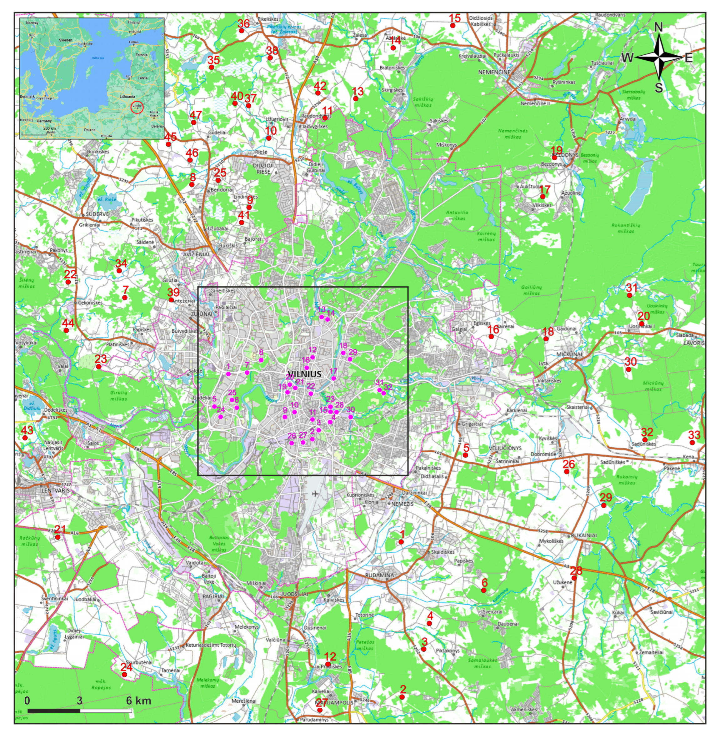
• Studying Quaternary geological maps and purposefully selecting topsoil sampling sites in the Vilnius peri-urban area considering different ages and genetic types of deposits, collecting composite samples, and determining different types of variables.
• Obtaining new information regarding the magnitude and variability of the variables and the correlation between their different types for identifying a preliminary list of influential non-elemental variables and potential reference elements (PREs) and adjusting this list after studying the clustering of basic variables selected, taking into account mineralogical groups of selected common minerals.
• Studying the influence of age, genetic type, and lithology of Quaternary deposits on topsoil variables and identifying which of them is the key property, determining whether BVs required for urban sites should be estimated using a subset of sites with relatively lower or with relatively higher levels of PHEs and PREs.
• Testing whether a cluster analysis dendrogram of samples compiled using basic variables is suitable for statistical site classification into BS and NBS and whether additional information about sites is helpful for selecting BS.
• Testing different variable type(s) for statistical site classification, followed by the estimation of BVs in the respective background subsets with the aim of proposing the most useful variables, i.e., reference variables.
• Comparing statistical site classifications based on the most useful variables determined in topsoil with two selected nonstatistical site classifications, one of which is based on the key property of Quaternary deposits while the other relies on the most useful non-elemental variables related to this property.

2.2. Sampling and Adjustment of Information about Properties of Quaternary Deposits in Sites

The selection of topsoil sampling sites in the peri-urban area of Vilnius was purposeful, with planning based on a geological map and proportional representation of the areas covered by different ages and genetic types of Quaternary deposits. The sites were chosen in shallow relief meadows, as far as possible from past or current urban activities (Figure 1). Each primary composite sample, weighing approximately 2.5–5 kg, consisted of five subsamples collected from the corners and center of a square measuring approximately 10 m × 10 m. The subsamples were mixed in a plastic bucket and quartered to reduce the mass of the final composite sample to around 2–3 kg. In total, 47 composite samples were collected.

Revised information about the properties of underlying Quaternary deposits in peri-urban sites was acquired from digital maps of the Lithuanian Geological Survey and their respective database [50] according to the coordinates recorded during sampling (

Table 1. Stratigraphy and lithology of underlying Quaternary deposits in the study sites and certain urban sites according to the Lithuanian Quaternary geological map.

Area	Age a and Genetic Type b	Sites and Lithology c
Peri-urban	gt II md	1 (gt), 2 (gt), 3 (gt), 4 (gt), 5 (gt), 6 (gt)
	g III gr and gt III gr	7 (gt), 8 (gt), 9 (gt), 10 (gt), 11 (gt), 12 (gt), 13 (gt), 14 (gt), 15 (gt), 16 (gt), 17 (gt), 18 (gt), 19 (gt), 20 (gt)
	f III gr and ft III gr	21 (sv), 22 (sg), 23 (sg), 24 (sg), 25 (sg), 26 (sv)
	lg III gr	27 (sf), 28 (sf), 29 (sf), 30 (sf), 31 (sf), 32 (sf), 33 (sf)
	gt III bl	34 (gt), 35 (gt), 36 (gt), 37 (gt), 38 9 gt)
	f III bl and ft III bl	39 (sg), 40 (sf), 41 (sv), 42 (sv)
	lg III bl	43 (cl), 44 (sm), 45 (cs), 46 (cs), 47 (cs)
Part of urban	ft II md	1 (sf), 2 (sv), 3 (sv), 4 (sv), 32 (sf)
	f III bl and ft III bl	5 (sv), 6 (sf), 7 (sv), 8 (sv), 9 (sf), 10 (sf), 11 (sg), 12 (sg), 13 (sv), 14 (sv), 15 (sf)
	a III bl	16 (sv), 17 (sf), 18 (sf)
	a IV	19 (sf), 20 (sf), 21 (sf), 22 (sf), 23 (sf)
	d IV	24 (sc), 25 (sc), 26 (sc), 27 (sc), 28 (sc), 29 (sc), 30 (sc), 31 (sc)

^a II md—Middle Pleistocene Medininkai, III gr—Late Pleistocene Grūda, III bl—Late Pleistocene Baltija, and IV—Holocene. ^b lg—proglacial glaciolacustrine, g—basal till, gt—marginal till, f—proglacial glaciofluvial, ft—marginal glaciofluvial, a—alluvial, and d—deluvial. ^c gt—glacial till, sg—gravelly sand, sv—various sand, sm—medium sand, sf—fine sand, cl—clay, cs—silty clay, and sc—clayey sand.

). Similar information, using coordinates, was also collected for 32 urban sites where topsoil geochemical investigations for monitoring purposes had been previously conducted most frequently (Figure 1 and Table 1).

2.3. Sample Preparation and Determination of Variables

Composite samples of topsoil were brought to the laboratory, where they were air-dried, quartered, and sieved through a 2 mm nylon sieve to produce representative portions of about 0.5–1.5 kg. Representative sub-portions were selected from each portion for all types of analysis. These sub-portions were further denominated as laboratory samples.

The procedure of preparing laboratory samples for X-ray fluorescence (XRF) analysis was as follows: (i) two independent laboratory subsamples (each being ≥ 5.0 g) were chosen and ground for 10 min at 27 Hz using a MM 400 mill with zirconium oxide grinding jars and grinding balls; (ii) then, 4.00 g of each powdered material was homogenized with 0.90 g of Licowax binder (dilution factor 0.816, as recommended by the equipment manufacturers) and pressed for 3 min using 15 kN (press PP15) to produce 32 mm diameter pellets.

The pellets were analyzed using the energy-dispersive XRF equipment Xepos HE (SPECTRO Analytical Instruments GmbH, Kleve, Germany) and TurboQuant (TQ) II calibration for the pressed pellets module, as specified by the manufacturer. The TQ method combines different procedures: calculation of the mass attenuation coefficient, using the extended Compton module, and a final calibration based on the fundamental parameter method. The advantages of the polarization method and TQ calibration method were described by Schramm and Heckel [51]. TurboQuant II, the latest modification of the TQ method intended for XEPOS HE, is offered by the manufacturer for samples with various matrices [52]. More detailed information on the analysis quality and detection limits is provided in [53]. A detailed description of the XRF conditions used was provided earlier [51]. Duplicates of the pressed pellets were analyzed twice to quantify the contents of the following 26 elements: Na, Mg, Al, Si, P, S, K, Ca, Fe, Ti, V, Cr, Mn, Co, Ni, Cu, Zn, Ga, As, Br, Rb, Sr, Nb, Mo, Ba, and Pb.

The compliance with quality assurance requirements was ensured in the following five aspects: (1) limits of detection (LOD), (2) levels of relative standard deviation (%RSD, see pages 8 and 25–28 in [54]) calculated for the data of analyzed duplicates, (3) participation in the International Soil-Analytical Exchange (ISE) program, (4) using the reference materials (RMs) and certified reference materials (CRMs), and (5) adjusting via recalibration procedures. Accordingly, (i) all analyte contents were higher than the respective lower LOD values (see in Table 2 in [53]); (ii) the %RSD values were 5.0%–7.0% for Na, S, V, Cr, Co, As, and Mo, while the values were below 5.0% for Mg, Al, Si, P, K, Ca, Fe, Ti, Mn, Ni, Cu, Zn, Ga, Br, Rb, Sr, Nb, Ba, and Pb; and (iii) averaged values of the duplicate measurements were adjusted via recalibration procedures using both a large number of RMs obtained during our laboratory’s participation (period 1998–2019) in ISE, organized by WEPAL [55], and CRMs intended for soils, such as NIST 2702, NIST 2704, NIST 2709, NIST 2711, and NIST 2782; CRM 277 and CRM 320; and DC73022 and DC73317a, as well as OKOOO201, OKOOO202, OKOOO203, OKOOO204, OKOOO301, OKOOO302, and OKOOO303. The used RMs and CRMs were prepared pari passu with our analyzed topsoil samples. Earlier, we mentioned these procedures in a series of publications including [3,56,57,58,59,60,61].

Grain size measurements were conducted using the Fritsch Laser Particle Sizer Analysette 22 MicroTec Plus, which was also employed in [62]. Loss-on-ignition (LOI) variables were determined via combustion until 550 °C (550′) and further combustion until 950 °C (950′) [63]. The quantitative assessment of the bulk mineralogical composition was carried out at Tartu University using the X-ray diffraction (XRD) method with a Bruker D8 Advance diffractometer equipped with CuKα radiation and a LynxEye positive 192 sensitive detector in the 2–70° 2 Θ range. The bulk mineralogical composition was characterized by the following 13 minerals: quartz, orthoclase, microcline, albite, anorthite, hornblende, muscovite, illite, kaolinite, chlorite, calcite, dolomite, and hematite.

2.4. Statistical Methods

The results that require special algorithms were obtained using the software STATISTICA, version 8 [64]. The following algorithms were employed: (1) identifying significant (p < 0.01) Spearman’s correlation coefficients (rS), (2) principal component analysis with varimax rotation, (3) hierarchical cluster analysis of variables with 1-rS distance measure and Ward’s method, (4) hierarchical cluster analysis of sites using Ward’s method and the city block distance measure between standardized variables, (5) hierarchical cluster analysis of site classifications using Ward’s method and the percent disagreement (PD) as the distance measure, (6) Mann–Whitney U-test for comparing two groups, and (7) H-test of the Kruskal–Wallis ANOVA with multiple comparisons for comparing more than two groups, taking into account two-sided significance levels with Bonferroni adjustment.

Microsoft Office Excel 2003 [65] was used to calculate robust coefficients of variation, determine BVs using the Median ± 2MAD method [36] (where MAD is median of absolute deviations from the median), compute certain indices, prepare most figures, except dendrograms, and reorganize data. Conditional color formatting, as described in [60], was performed using Excel in Microsoft 365 [66].

3. Results

3.1. Topsoil Variables

The arrangement of major elements in descending order of mean or median contents is as follows: Si > Al > K > Fe > Ca > Mg > Na > Ti (

Table 2. Statistical estimates of elemental contents and grain size and loss-on-ignition variables.

Groups of Variables	Variable a	Mean	CV (%) b	RCV (%) c	LQ d	Median	UQ e
Major elements	Al	27,331	22.2	11.1	23,383	26,900	28,714
	Ca	5787	72.3	23.9	3323	4287	5309
	Fe	10,160	40.6	22.8	7206	9071	11,322
	K	14,495	19.6	9.11	12,856	14,249	15,308
	Mg	4274	58.7	32.6	2480	3341	5454
	Na	1995	20.0	17.6	1610	1993	2300
	Si	363,436	7.18	3.82	344,283	371,807	383,242
	Ti	1365	29.7	15.0	1145	1291	1486
Minor or trace elements	As *	2.57	60.0	41.9	1.45	1.84	3.48
	Ba *	302	13.5	10.5	268	302	330
	Co *	3.69	40.3	25.0	2.45	3.52	4.26
	Cr *	18.0	40.3	24.2	12.8	16.2	21.8
	Cu *	13.0	34.7	20.2	10.1	12.4	15.1
	Mo *	0.60	44.9	38.6	0.34	0.55	0.78
	Ni *	11.3	35.0	19.6	8.45	10.5	12.7
	Pb *	17.5	11.9	6.76	16.2	17.1	18.8
	V *	42.5	33.4	21.9	32.4	39.9	49.2
	Zn *	36.8	32.1	16.3	29.3	33.1	41.0
	Br	2.78	26.3	16.4	2.23	2.75	3.14
	Ga	6.16	26.1	12.5	5.07	6.01	6.60
	Mn	302	34.8	20.6	243	297	362
	Nb	6.22	26.6	14.9	5.35	5.89	6.84
	P	729	22.9	18.1	598	718	843
	Rb	48.9	23.6	11.5	42.6	47.9	51.4
	S	191	60.9	30.1	114	155	219
	Sr	72.3	11.1	6.52	67.1	71.6	75.8
Grain size fractions, %	<2′ f	14.6	54.4	29.2	9.69	11.9	17.1
	2–63′ g	43.1	27.6	17.0	37.4	43.7	51.1
	<63′ h	57.7	26.9	14.4	50.7	56.3	65.0
	>63′ i	42.3	36.8	18.7	35.0	43.6	49.3
Loss-on-ignition (LOI) variables, %	550′ j	3.29	33.8	19.4	2.58	2.89	3.77
	950′ k	0.46	79.9	35.0	0.23	0.34	0.52

^a Mean, median contents, and quartiles of elements are in mg kg⁻¹. PHEs are denoted by an asterisk. ^b Coefficient of variation. ^c Robust coefficient of variation. ^d Lower quartile (25th percentile). ^e Upper quartile (75th percentile). ^f Clay fraction. ^g Silt fraction. ^h Clay and silt (fine) fraction. ⁱ Sand fraction. ^j LOI at 550 °C. ^k LOI at 950 °C.

). In this group, Si has the lowest variability, while Mg and Ca have the highest. The decrease in PHEs based on their mean or median contents is as follows: Ba > V > Zn > Cr > Pb > Cu > Ni > Co > As > Mo. Among them, Pb has the lowest variability and As has the highest. According to the descending mean values, presumably nonharmful minor or trace elements are arranged as follows: P > Mn > S > Sr > Rb > Nb > Ga > Br. Strontium has the lowest variability, while S has the highest.

The dominant fraction is 2–63′, followed by >63′, while the <2′ fraction percentage is the lowest. However, the dataset is more homogeneous, according to the 2–63′ and >63′ percentages, than according to the <2′ percentage. The mean and median values of 550′ exceed the respective values of 950′, but the variability of 550′ is lower than that of 950′.

The arrangement of the 13 minerals according to descending mean percentages is as follows: quartz > illite > orthoclase > albite > microcline > anortite > chlorite > kaolinite > muscovite > dolomite > hornblende > calcite > hematite (

Table 3. Topsoil bulk mineralogical composition (%) and its variability (%) in peri-urban sites.

Minerals, % (Abbreviations)	Mean	CV a	RCV a	10th b	LQ	Median	UQ	90th c
Quartz (Q)	71.5	10.0	4.81	63.3	69.5	72.0	75.6	80.1
Illite (IT)	7.09	54.1	28.5	3.66	4.58	6.03	7.97	12.2
Orthoclase (OR)	6.03	22.7	12.7	4.80	5.18	5.74	6.79	7.97
Albite (AL)	4.09	17.8	13.3	3.10	3.58	5.46	4.63	4.96
Microcline (MC)	4.02	53.4	58.1	1.74	1.93	4.10	6.04	6.47
Anorthite (AN)	1.89	25.7	20.5	1.31	1.47	1.85	2.27	2.62
Chlorite (CH)	1.56	59.2	46.4	0.65	0.77	1.50	1.98	2.72
Kaolinite (KA)	1.29	64.4	37.0	0.25	0.48	1.30	1.69	2.19
Muscovite (MU)	0.90	83.3	67.7	0.03	0.21	0.89	1.37	1.86
Dolomite (DO)	0.50	113.6	45.9	0.14	0.19	0.42	0.48	1.14
Hornblende (HO)	0.48	42.6	38.7	0.22	0.30	0.35	0.65	0.77
Calcite (CA)	0.35	92.7	75.3	0.06	0.08	0.25	0.53	0.68
Hematite (HE)	0.26	35.0	29.0	0.17	0.19	0.23	0.35	0.39

^a Most abbreviations of statistical estimates are in Table 2. ^b 10th percentile. ^c 90th percentile.

). Quartz has the lowest variability compared to the other minerals. Most feldspars (orthoclase, albite, and anorthite) have relatively lower variability compared to illite and other minerals.

Nine common minerals, known as representatives of terrigenous or carbonate rocks, were selected for factor analysis (

Table 4. Factor-loading matrix of selected minerals in topsoil.

Factor	IT a	KA	MU	OR	Q	DO	CA	AL	AN	Expl. Var, % b
F1	0.95 *	0.89 *	0.77 *	0.67 *	−0.98 *	0.05	−0.22	0.10	−0.03	41.8
F2	0.01	−0.22	−0.22	0.05	−0.03	0.95 *	0.91 *	0.17	−0.15	20.9
F3	0.18	−0.20	−0.33	0.36	0.17	−0.05	0.02	−0.63 *	−0.84 *	16.1

^a Abbreviations of minerals are as in Table 3; they are listed in descending order of their significance (p < 0.01), denoted by asterisks, of loadings on F1, followed by F2 and, finally, F3. ^b Percentage of total variance explained by the factor.

). Five of them have significant (p < 0.01) loadings on the first factor (F1), namely illite, kaolinite, muscovite, orthoclase, and quartz. This factor exhibits the highest variability. The other two factors, F2 with significant loadings of dolomite and calcite and F3 with significant loadings of albite and anorthite, have lower variability.

3.2. Correlation between Different Types of Variables in Topsoil

The Spearman’s correlation coefficients of elemental contents with non-elemental variables (Table S1) are valuable for determining which of the latter are more suitable to be used in site classification. Based on their correlation with PHEs, the non-elemental variables can be categorized into three groups: (i) influential, which include clay (<2′), sand (>63′), and fine (<63′) fractions; 950′; illite, kaolinite, orthoclase, and quartz; (ii) partly influential, consisting of silt (2–63′), muscovite (MU), and 550′; (iii) weakly influential, such as dolomite, calcite, albite, and anorthite. Influential non-elemental variables exhibit a significant (p < 0.01) relationship (either positive or negative) with all PHEs. Four minerals in this influential group have significant loadings on F1 (Table 4) and are also significantly correlated with other non-elemental variables (Table S2).

In addition, all eight influential non-elemental variables consistently show significant (p < 0.01) correlations with nine presumably nonharmful elements, i.e., Al, Fe, K, Mg, Si, Ti, Ga, Rb, and Nb (Table S1). They will be referred to as potential reference elements (PREs). The significant correlation of influential non-elemental variables with both all of the PHEs and the nine PREs indicates that their selection for site classification is justified. This also suggests that the nine PREs can potentially replace influential non-elemental variables.

Partly influential variables (2–63′, MU, and 550′) are also quite suitable for site classification, as they exhibit a significant (p < 0.01) correlation with a subset of PHEs (Table S1). Furthermore, the significant correlation of 2–63′ and MU with all PREs indicates that these variables are more suitable for site classification than 550′, which correlates with only seven PREs.

The correlation of weakly influential non-elemental variables (four minerals) with PHEs is mostly insignificant, with only three exceptions: Ba–albite and Pb–albite show positive correlations, and Ba–calcite shows a negative correlation. None of these minerals have a significant correlation with PREs. This result suggests that they are the least suitable for site classification.

3.3. Grouping of Different Types of Variables

The contrast observed among variables of certain types—specifically, grain size, minerals, or elements—and expressed through significant negative correlation proves that they are highly beneficial for site classification. This is demonstrated in dendrograms of basic (40 or 39) variables (Figure 2). Considering the partial overlap between fractions 2–63′ and <63′, only <63′ was selected for its stronger correlation with PHEs and PREs (Table S1). Influential non-elemental variables are in different branches: significantly positively correlated quartz and sand fractions (>63′) are in the upper, while closely positively intercorrelated clay (<2′) and fine (<63′) fractions and illite, orthoclase, and kaolinite (Table S2) are in the lower. Muscovite, partly influential, contributes to the lower branch. If 950′ is included, it is also placed in the lower branch (Figure 2a). However, 550′, which has the highest positive correlation with S and Br (Table S1), is in the upper branches due to insignificant correlations with minerals and clay fractions.

Eight PHEs are positioned in the lower branches. The placement of Pb and Ba in the upper branches is attributed to their significant correlation with albite and also because Pb has the highest positive correlation with 550′ among the PHEs.

All PREs, except Si, closely correlated with the sand fraction and quartz, are in the lower branch due to correlations with clay; fine fractions; and four minerals: IT, KA, MU, and OR (Table S1).

The location of Ca is different; if 950′ is included (Figure 2a), the element is in the lower branch, although its correlation with influential non-elemental variables <2′, MU, KA, and OR is insignificant (Table S1). The reason is that Ca is significantly negatively correlated with the sand fraction (>63′) and, therefore, significantly positively correlated with the fine fraction (<63′). Moreover, Ca and Mg are somewhat separated from most variables of the lower branch, since both have significant and the highest positive correlation with 950′ in comparison with the other non-elemental variables (Table S1). However, 950′ is significantly positively correlated not only with IT, KA, MU, and OR but also with the weakly influential dolomite (Table S2), although this correlation is lower. Only Ca has a significant correlation with dolomite but not Mg (Table S1). Therefore, if 950′ is included, both elements are not in the same branch as dolomite and calcite (Figure 2a); otherwise, Ca is closer to carbonates, while Mg is closer to clay minerals (Figure 2b).

The correlation of Ca (Table S1) and 950′ (Table S2) with minerals attributed to different factors (Table 3) confirms that it was logical to avoid including Ca in the PREs and raises doubt about the need for the 950′ variable in site classification, as the interpretation of the results might become more complicated. The fact that Mg is associated with Ca and 950′ also suggests eliminating Mg from the nine PREs.

3.4. Influence of Properties of Quaternary Deposits on Topsoil Variables

To analyze the influence of age, genetic type, and lithology of Quaternary deposits on topsoil variables, sampling sites were classified into three groups in three ways: (i) sites on deposits of Medininkai, Grūda, and Baltija ages; (ii) sites on glacial, glaciofluvial, and glaciolacustrine genetic types; and (iii) sites on sandy, clayey deposits, and glacial till.

The question of whether age or genetic type of Quaternary deposits has a greater influence on topsoil variables is complicated. We attempted to address this by fixing one of the two properties to judge the other when possible.

The influence of the age of Quaternary deposits on topsoil variables appeared to vary depending on the genetic type (Table S3). It was noticeable in sites on glacial deposits, where the number of variables with statistically significant (p < 0.05 or even p < 0.01) age-related differences was seven (Fe, Mg, Ni, P, <2′, illite, and 950′), but invisible in sites on glaciofluvial deposits and clearly expressed in sites on glaciolacustrine deposits, where this number was 25, including all grain size fractions; five minerals that significantly load F1 (Table 3); seven PHEs; and seven PREs (Al, Fe, K, Ti, Ga, Nb, and Rb).

The influence of Quaternary genetic type on topsoil variables could not be studied for the Medininkai age, as all sampling sites were on glacial deposits. The results regarding other ages were also controversial. In sites on Grūda age deposits, the influence of genetic type was low, with only four slightly significant differences: Ca, Sr, albite, and anorthite—elements not attributed to PREs and minerals related to the least variable factor, F3 (Table 4). Meanwhile, in sites on Baltija age deposits, this influence was found to be much greater, with 19 statistically significant differences, including most grain size fractions, two clay minerals, five PREs, six PHEs, 550′, and S and Br, which are correlated with it.

Such controversial results suggest analyzing seven groups according to a combination of age and genetic type. In this case, much more (27) statistically significant differences in topsoil variables are revealed, including <2′ and 2–63′ fractions, five minerals with significant loadings on F1, seven PREs, six PHEs, and both LOI variables.

However, the classification of sites according to the lithology of Quaternary deposits demonstrates the highest influence, as reflected in 34 from 41 tested topsoil variables, including almost all elements (Figure 3); all four grain size fractions; 550′; and six minerals: IT, KA, OR, Q, DO, and AL (Table S3). It is the only one that reveals significant differences in the topsoil content of Si and the percentage of dolomite. Lithology is related to both age and genetic type and, therefore, inevitably has the highest influence on topsoil variables. Using classification according to this key property, the p-values of multiple comparisons show that most of the elements have a statistically higher (p < 0.05 or p < 0.01) mean rank in sites on clayey deposits than on sandy deposits or glacial till (Figure 3).

3.5. Reflection of Quaternary Lithology and Topsoil Texture in Dendrograms of Sites

Since the classification of sites according to the lithology of Quaternary deposits provides the highest number of statistically significant differences in the values of topsoil variables (Table S3), and this property is related to the proportion of sandy and clayey components in samples (Figure 3), it might be presumed that sites will be clustered according to this feature. However, the dendrogram compiled using the basic 40 variables demonstrates that the reflection of this feature is far from ideal (Figure 4a): (i) 18 sites on sandy Quaternary deposits are distributed not only in clusters C1 (n = 2) and C2 (n = 16) but also in C3 (n = 9) and C4 (n = 1); (ii) 20 sites on glacial till are in almost all clusters, except C1; and (iii) four sites on clayey deposits are in the C5 (n = 3) and C4 (n = 1) clusters. An analogous result is when clustering is without a 950′ variable (Figure 4b).

On the other hand, the clustering of sites is a useful tool for determining subsets with different levels of PHEs or PREs, selecting a background subset (BS), and estimating the respective BVs. This becomes evident after applying conditional color formatting to the rearranged data matrix (Figure 5), where the basic 39 variables are sorted as shown in Figure 2b and the sites as in Figure 4b. The downward decrease in Si, quartz, and the sand fraction in five clusters of sites is visible. On the contrary, the contents of most PREs (Al, Fe, K, Rb, Ga, Ti, and Nb) and PHEs (Cr, Ni, Co, As, Zn, Cu, and V) increase in this direction. The shading of their values mainly corresponds to that of illite, <2′, and 2–63′ fractions.

Since urban sites of Vilnius are often on sandy Quaternary deposits (Table 1), the BS should include clusters mainly with green-shaded values of the aforementioned elements, i.e., the 18 uppermost samples.

The insufficient reflection of the Quaternary lithology in the dendrograms of the cases can be explained by pedogenic processes, which influence the absence of a one-to-one correspondence between the Quaternary lithology and topsoil texture classes (Figure 6). However, the greater part of topsoil on sandy Quaternary deposits is either sandy loam (SL) or loam (L).

Topsoil texture classes are reflected in clusters better than Quaternary lithology. For example, both background subsets in Figure 4 include only sites with a coarser texture, i.e., all SL samples and part of the L samples. The advantage of the coarser texture SL + L criterion is confirmed by the decrease in relative medians of Si and the tendency of an increase in 23 other basic elements (except Na and P) in the sequence of topsoil texture classes: SL < L< SiL < finer texture (Figure 7).

3.6. Clusters Distinguished Using a Certain Type of Variables or a Combination of Clay Fraction and Soil Organic Matter Indicator

Is the inclusion of all variables in the cluster analysis necessary for reasonable site classification and the selection of BS? It is quite possible that some of them are redundant and distort the clustering version that is most helpful for the choice of BS. Moreover, it might be useful to determine the relative role of the different types of variables in site classification.

Using solely grain size fractions, the BS is formed from C1 and C2, with 21 sites in these two clusters (Figure S1a). This version well reflects the topsoil texture classes: all the SL samples and about half of the L samples are in these clusters; moreover, C1 consists solely of SL. Meanwhile, if the variables <2′ and 550′ are used (Figure S1b), the BS contains more (27) sites in the C1 and C2 clusters. However, this clustering version insufficiently reflects texture classes: (i) not all SL sites are in the BS, and (ii) the BS includes not only SL and L but also silt loam (SiL). Both versions in this figure are similar according to the same scheme of the amalgamation of clusters: (C1–C2)–[(C3–C4)–C5].

A comparison of four versions of clustering using solely elemental contents was conducted (Figure S2). The versions using all 26 elements (Figure S2a) or only eight PREs, i.e., Al, Fe, Ga, K, Ti, Nb, Si, and Rb (Figure S2b), are similar according to the number of sites included in the BS and the scheme of the amalgamation of five clusters, i.e., [(C1–C2)–(C3–C4)]–C5. But the b-version better reflects the texture classes: (i) BS does not include the SiL sample, and (ii) SL dominates in the C1 cluster, while L dominates in the C2 cluster. The version based on 11 elements (Figure S2c) when S, Br, and P, which are related to 550′ (Figure 2a), are added to PREs shows that the BS includes the same 19 sites as the dendrogram compiled using only eight PREs (Figure S2b), despite the arrangement in the C1 and C2 clusters of two dendrograms slightly differing. The version based on 10 PHEs (Figure S2d) demonstrates that the BS has more sites (28) from the C1 and C2 clusters; moreover, it includes almost all sites from the BS of the a-version, except site 24. But in the d-version, the relation of the BS to a coarser topsoil texture is weaker, since it includes two silt loam (SiL) samples.

Two versions of clustering using only mineralogical data (Figure S3a,b) are similar according to the same number of sites in the BS and the amalgamation scheme of clusters, i.e., (C1–C2)–[C3–(C4–C5)]. But both versions insufficiently reflect the soil texture classes, and it is difficult to judge which version is better due to controversial results: (i) in the a-version, the BS includes four SiL samples, while, in the b-version, there are only three; (ii) in the a-version, BS includes eight SL sites, while, in the b-version, there are only seven. The fact that, in the b-version, the CT value of C3 is higher than that of C2 causes doubt regarding whether C1 + C2 or C1 + C3 should be included in the BS. Therefore, solely mineralogical data are less helpful for site classification than grain size fractions or elemental contents.

3.7. Comparison of Eight Site Classifications into Background Subsets and Non-Background Subsets

There are two identical site classifications to background subset BS and non-background subset NBS: using 11 elements (Figure S2c) and using PREs (Figure S2b). This means that, in our study area, S, Br, and P, which are related to the 550′ variable, have a much lower influence on site classification in comparison with Al, Ga, Fe, K, Nb, Rb, Si, and Ti.

All eight versions of site classification are rather similar: six sites, i.e., 2, 8, 18, 19, 27, and 41, are always in BS, while 12 sites, i.e., 10, 13, 21, 28, 33, 34, 36, 39, 43, 45, 46, and 47, are never in it (Table S4). Six sites, which are in each BS, have coarser texture: five are attributed to SL and only one to L. Meanwhile, Quaternary deposits in BS sites are variable: four sites are on glacial till and two on sand; their ages and sedimentation types are also different.

The dendrogram of eight site classifications using the percent disagreement (PD) (Figure 8) as a distance measure demonstrates that two pairs of versions are most similar: (i) using nine minerals and using five minerals and (ii) using three grain size fractions and using eight PREs (or PREs with S, Br, and P).

Both pairs have PD = 0.04, which is the lowest (

Table 5. The percent disagreement between eight versions of site classification into BS and NBS.

Variables Used in Cluster Analysis	<2′, <63′ and >63′	8 PREs	26 Elements	40 Variables	<2′ and 550′	10 PHEs	9 Minerals c	5 Minerals d
<2′, <63′ and >63′ a	0.00	0.04	0.06	0.09	0.38	0.19	0.26	0.26
8 PREs a	0.04	0.00	0.06	0.04	0.38	0.23	0.26	0.30
26 elements a	0.06	0.06	0.00	0.06	0.36	0.17	0.23	0.28
40 variables a	0.09	0.04	0.06	0.00	0.38	0.23	0.30	0.34
<2′ and 550′ b	0.38	0.38	0.36	0.38	0.00	0.23	0.47	0.51
10 PHEs b	0.19	0.23	0.17	0.23	0.23	0.00	0.36	0.36
9 minerals b	0.26	0.26	0.23	0.30	0.47	0.36	0.00	0.04
5 minerals b	0.26	0.30	0.28	0.34	0.51	0.36	0.04	0.00

^a Associated group (AG) of site classifications. ^b Less-associated group (LAG) of site classifications. ^c IT, KA, MU, OR, Q, DO, CA, AL, and AN. ^d IT, KA, MU, OR, and Q. The arrangement of versions is the same as in Figure 8.

). The first pair shows the natural similarity of site classifications using the same variable type; meanwhile, the second pair demonstrates similarity when using different types of variables.

The latter result is very useful for application in practice, since it indicates that PREs can substitute for grain size fractions that describe the topsoil texture. Moreover, the fact that site classification using 40 basic variables is very similar to that using eight PREs (PD = 0.04) demonstrates the efficiency of PREs among all the variables.

Four site classifications, i.e., using grain size variables, eight PREs, 26 elements, and 40 basic variables, are most similar and form an associated group (AG) (Figure 8). All 17 sites in BS when using 40 variables (Figure 4a) are also in background subsets of the other three versions, but the latter three versions include some additional sites (Table S4).

Meanwhile, two site classifications using mineralogical data are less similar to the AG versions (PD > 0.23) (Table 5); the same results are found in the site classification using <2′ and 550′ (PD > 0.36). Only the site classification using 10 PHEs is slightly closer (PD range is 0.17–0.23). We can entitle these four versions as less-associated group (LAG). Compared to the members of LAG, site classifications of AG result in a higher contrast between NBS and BS (Table S5): (i) contrast ratios (CR), i.e., the median in NBS divided by the median in BS, are slightly higher for 23 basic elements (except Si, Na, and P), and (ii) the significance level of differences is higher, especially for PREs and As, Co, Cr, Cu, Ni, and Pb.

Site classification using 10 PHEs is most similar to the version using 26 elements (PD = 0.17). Its lower similarity to versions using grain size fractions (PD = 0.19) or eight PREs (PD = 0.23) can be explained by the influence of topsoil organic matter on the contents of some PHEs. This presumption is confirmed by the clustering of site classification using 10 PHEs with that using <2′ and 550′ variables (Figure 8) with PD = 0.23 (Table 5). Moreover, site classification using 10 PHEs is even less similar to both versions of site classification using mineralogical data (PD = 0.36).

Although the inclusion of mineralogical data among the 40 variables does not decrease similarity with site classification using 10 PHEs (PD = 0.23), it seems that the determination of bulk mineralogy is redundant. The lower contrast between BS and NBS when using solely mineralogical data for site classification (Table S5) confirms this presumption.

To conclude, two versions of site classification based on elemental contents are advantageous: (i) using 26 elements and (ii) using eight PREs. Both ensure a less expensive estimation of BVs, since the determination of grain size fractions and LOI variables is not necessary. The first version uses a wide elemental group, including not only PHEs but also PREs, which are necessary for the calculation of EFs. It has a rather low PD = 0.06 with all versions in AG and relatively the lowest PD = 0.17 with the version using 10 PHEs. However, its drawback can manifest when elevated contamination by PHEs exists in the peri-urban area. In this case, although PHEs are determined, their inclusion among other elements can distort clustering, so it is better to rely on site classification using solely PREs. Greater similarity with site classification based on grain size or even all 40 variables (PD = 0.04) confirms the advantage of this version, although it is slightly less similar to the version based solely on PHEs (PD = 0.23).

3.8. Comparison of Background Values (BVs) Obtained from Eight Background Subsets (BSs)

Even if cluster analysis enables the selection of BSs, it can still include anomalies of some elements. Therefore, it is necessary to eliminate them. Of course, they can be identified by the conditional color formatting of 39 variables (Figure 5) and respective sites removed for further estimation of BVs according to the remaining samples. For example, it seems that, according to the non-elemental variables, there are two anomalous samples: (i) 20 (elevated values of <63′ resulting in SiL texture and also 550′, IT, and OR) and (ii) 31 (increased values of CA, DO, and 550′).

But we preferred to use the Median ± 2MAD method, because it performs individual elimination of anomalies for each element. In this way, the refined background subsets (BSr) were obtained and BVs were estimated as their medians (Table S6). The number of sites in the BSr is different for each element but is always lower or equal to the number of sites in the initial BS.

For most elements (16 out of 26), the eight versions of refined background subsets are similar (p-value of H-test exceeds 0.05), while statistically significant differences exist only for ten elements (Table S6). However, four of these elements—Al, Ti, Br, and Nb—have only slightly significant (p < 0.05) differences, and multiple comparisons do not show statistically significantly different pairs of versions. Such pairs exist only for six elements: K, Rb, Co (p < 0.01), Ba, Cu, and Ga (p < 0.05). The greatest number of statistically significant differences is between BSr based on <2′ and 550′ variables and based on other versions. The version based on PHEs results in additional statistically significant differences: two for K and one for Ga. But there are no statistically significant differences between refined background subsets of AG site classifications.

Most similar AG site classifications (Figure 8) result in similar BVs (Table S6). In this group, the ratio of maximum to minimum BV (MaxMin) for 23 elements is lower than 1.1, with only three higher values, namely for Co (1.2), Cu (1.2), and Mo (1.3). Meanwhile, LAG site classifications are less similar; therefore, MaxMin < 1.1 only for 14 elements, while, for 10 (Fe, K, Mg, As, Cu, Ni, V, Br, Ga, and Rb), it is within the interval 1.1–1.3, and for two, it is even higher, namely for Co (1.4) and S (1.3). The MaxMin values calculated according to eight site classifications are within the following intervals: ≤1.1 for 7 elements (Ca, Si, Pb, Zn, Mn, P, and Sr); 1.10–1.3 for 12 elements (Al, K, Na, Ti, As, Ba, Cr, Ni, V, Br, Nb, and Rb); and ≥1.3 for 7 elements, namely Fe (1.3), Mg (1.4), Co (1.7), Cu (1.4), Mo (1.3), Ga (1.3), and S (1.3). The wider range of MaxMin calculated according to eight site classifications indicates that the main differences are between versions from AG and LAG. According to multiple comparisons, the greatest number of statistically significant differences is between two background subsets: (i) based on the <2′ and 550′ variables and (ii) based on 40 basic variables (Table S6). In comparison with a version of 40 variables, the BVs based on site classification using the <2′ and 550′ variables are higher for most elements, except Na, Si, S, and P. Moreover, for Co, Cu, Mo, and Ga, the respective ratios of BVs are the highest.

4. Discussion

4.1. Mineralogical Specificity of the Study Area

Due to challenges in finding XRD-determined published topsoil bulk mineralogical results in neighboring countries, a comparison of our data was conducted with the results of soil analyses in two continental-scale transects across the United States and Canada [67], where mineral soil was sampled not only from the A-horizon but also deeper [68].

The main difference from the American results is a much higher percentage of quartz, orthoclase, and plagioclases in Vilnius peri-urban topsoil (Table 3). The mean value of quartz is 1.8 times, of orthoclase is 1.7 times, and of plagioclases is 1.5 times higher. Meanwhile, in the American A-horizon and in deeper soil, the mean values of quartz and orthoclase are even below the respective 10th percentiles of data around Vilnius (Table 3).

In contrast, the topsoil in our study area is deficient in many other minerals, as demonstrated by their arrangement based on decreasing ratios obtained by dividing the mean values in American soil from the A-horizon [67] by the respective mean values around Vilnius (Table 3): calcite (13) > kaolinite (4.7) > dolomite (3.2) > muscovite (2.8) > chlorite (1.9) > microcline (1.6). In both the A-horizon and deeper soil of the American transects, the mean values of these minerals, except for dolomite, exceed the 90th percentiles in the Vilnius surroundings (Table 3). The sum of the mean values of illite, kaolinite, chlorite, and muscovite, i.e., minerals attributed to layer silicates (phylosilicates) [69], in topsoil around Vilnius is 1.6 times lower than in the American A-horizon.

The main mineralogical similarity between the two areas lies in the percentage of illite, as its mean values in the American A-horizon and deeper soil fall within the interval from the 10th to 90th percentile of our data. Based on this criterion, the topsoil of the two areas is also comparable in the hornblende, hematite, dolomite, and albite percentages.

Comparison with highly developed soils of Central Spain [70] also confirms that topsoil around Vilnius is enriched in quartz; its mean percentage is 1.2 times higher. Additionally, there are 5.5 times more feldspars but 3.3 times fewer phylosilicates.

4.2. Relationship of Minerals with Grain Size and Elemental Contents

Quartz, constituting up to 95% of quartz in the sand [71], naturally shows a significant positive correlation (0.70) with the >63′ fraction (Table S2). The relationship extends to Si (0.71) being a constituent of quartz. Similarly, albite is the only mineral with a significant correlation with Na (0.48) (Table S1). Both results are analogous to those in the American soil A-horizon, where the Si–quartz relationship has an r² value of 0.74 and the Na–plagioclases correlation is 0.89 [67]. Clusters like quartz–sand–Si and Na–albite–anorthite include different types of variables (Figure 2).

In the peri-urban topsoil of Vilnius, quartz is about 2.5 times more abundant than the sum of the other minerals, while, in American soil, it is only two times [67]. Quartz plays a high role in the topsoil of the Netherlands as well [71].

The increase in quartz and the sand fraction (>63′) inevitably leads to a decrease in the fine fraction (<63′) and its constituents, namely clay and silt fractions, as well as the minerals accumulating in them. In our study, four minerals (illite, kaolinite, muscovite, and orthoclase) exhibit significant positive loadings on F1, contrasting with the significant negative loading of quartz (Table 4). Almost all elements, except Na, Si, Br, P, and Sr, also exhibit a significant negative correlation with quartz (Table S1), indicating that it acts as a diluent agent for their concentrations and background levels.

It is natural for illite and kaolinite, acknowledged representatives of clay minerals, to accumulate in the <2′ fraction, resulting in the highest significant correlation coefficients with it (Table S2). However, in topsoil around Vilnius, both of these minerals are also related to the 2–63′ fraction, albeit with lower rS compared to <2′ (Table S2). A possible explanation can be inferred from a study on soils in Central Spain, which demonstrates that these minerals are also present in fine silt, although with a lower percentage than in the clay fraction [70].

The contents of most elements, except Na, Si, Br, Mn, P, S, and Sr (Table S1), are significantly positively correlated with both clay minerals. An analogous finding was obtained in the study of soil in Spain [70], where phylosilicates and Al, Fe, V, Cu, Cr, Zn, and Ni form the highest positive loadings on the first most variable factor, while quartz and Si form the highest negative loadings. Our study demonstrates that elements are more strongly correlated with illite than with kaolinite (Table S1). The explanation is a higher specific surface area of illite (10–100 m²/g) in comparison with kaolinite (5–40 m²/g) [69]. Therefore, the adsorption of PHEs on illite is more obvious. An additional explanation is from the following facts about this mineral: (i) it has more element constituents in its formula, i.e., not only Al but also Mg, Fe, and K; (ii) it is a 2:1 type layer silicate but not 1:1 type; and (iii) “its tetrahedral sheet has more negative charge” because 20% of Si atoms are replaced by Al [69].

While feldspars are generally recognized as a group from which clay minerals form through hydrolysis [69], plagioclases (albite and anorthite) stand out due to their lack of significant correlation with fine fractions (Table S2). Furthermore, their abundance is lower compared to orthoclase (Table 2), which is similar to the lower mean of albite compared to orthoclase in the American soil A-horizon [67]. This suggests that plagioclases weather much more rapidly, a notion supported by observations of natural soil demonstrating a more rapid weathering of albite compared to K-feldspar [72]. Plagioclases and clay minerals may undergo separation and accumulation in different grain size fractions. This could explain the absence of a correlation between albite or anorthite with clay and silt fractions (Table S2), as well as the fact that plagioclases contribute significantly to the least variable mineralogical factor, F3 (Table 4). Consequently, in addition to Na, only a few elements exhibit a significant correlation with albite (Ba, Mn, Pb, and Sr) or anorthite (Sr) (Table S1).

During weathering, feldspars function as the primary minerals for both illite and kaolinite [69]. Therefore, the correlation of orthoclase with clay and silt fractions is quite natural. The higher percentage of feldspars in two silt fractions compared to the clay fraction in soil from Spain [70] suggests that this mineral should be correlated primarily with silt. A higher correlation of orthoclase with the clay fraction (Table S2) may be indirect, given its correlation with illite, known as a modified weathering product not only of feldspars but also of muscovite [69]. Muscovite, representing mica, i.e., a layered silicate, correlates with the <2′ fraction but not with the silt fraction (2–63′).

The mean values of dolomite and calcite are even lower than those of plagioclases (Table 2). Carbonate minerals have significant loadings on F2, which is also less variable than the F1 factor (Table 4). Their correlation with grain size fractions is insignificant (Table S2), and the influence on elemental contents is negligible (Table S1). The fact that only Ca is significantly correlated with dolomite (Table S1) suggests that Mg is mainly related to clay minerals, muscovite, or orthoclase. This presumption is confirmed by the table with the most common minerals in the Netherlands, where Mg is shown as a minor component in illite, muscovite, and alkali felspars [71].

4.3. Correlation of LOI Variables with Other Variables

The correlation between minerals and LOI variables differs: 950′ is significantly correlated with all minerals that load F1 significantly, as well as with dolomite; meanwhile, 550′ shows a correlation only with illite (Table S2).

In sediment analysis, both LOI variables have been in use for a considerable time [73,74] and currently assist us in paleoclimate reconstruction [75], while, in soil studies, mainly 550′ or organic carbon variables are employed [76,77] and are helpful as predictors of BVs for PHEs [38]. However, the variable 950′ might also be valuable for soil geochemical research, considering two important aspects of carbonates [78]: (i) coprecipitation of trace elements with incorporation into the structure of these minerals and (ii) precipitation of Fe and Mn oxides onto carbonates, thereby increasing the sorption of trace elements. In soils rich in CaCO₃, the hydrated hydroxides and insoluble carbonates of metals easily form [79].

Applying the LOI method for the assessment of inorganic carbon was successful in arid soils [80]. Meanwhile, our study shows that, despite the existence of the Ca–Mg–950′ cluster in the lower branch of the dendrogram (Figure 2a), the 950′ variable is a poor indicator of carbonates in the topsoil. A couple of facts contribute to this doubt: (i) an insignificant correlation of this variable with calcite (Table S2), leading to the separation of the three aforementioned variables from both carbonate minerals located in the upper branch, and (ii) an even higher positive relationship of 950′ with clay minerals (IT and MU) (Table S2). This can be explained by the finding that the increase in 950′ values may be due to the loss of some volatile noncarbonate components, especially lattice water in clays [74]. Experiments conducted by researchers on the thermal decomposition of illite have shown that the gradual removal of the hydroxyl groups from its tetrahedral sheet continues up to 850 °C [81]. The higher correlation of the 950′ variable with clay minerals than with carbonates in our topsoil also explains its significant relationship with the clay fraction (0.80), silt fraction (0.46), and fine fraction <63′ (0.75), as well as with muscovite and orthoclase, which directly associate with clay minerals in F1 (Table 4). The elements that have a significant correlation with 950′ are the same as those closely related to the clay fraction and include all PHEs; the only difference is that 950′ is additionally related to Ca and Sr (Table S1).

A possible explanation for the significant correlation of 550′ with illite (Table S2) is that this mineral tends to accumulate in clay fractions, where an increase in organic matter is commonly observed [69]. Clays are known to stabilize soil organic matter [82], suggesting a correlation between them. However, our present study shows that the 550′ variable has an insignificant correlation with the clay fraction (rS = 0.12) but a significant correlation with silt (rS = 0.70). Similar results were obtained in our earlier investigations of minerogenic topsoil around Vilnius [40], as well as by researchers studying topsoil in Spitsbergen [83].

Despite the insignificant correlation between 550′ and <2′ in our study, a more pronounced influence of organic matter in the clay fraction on the contents of most PHEs is evident. This is observed for As, Cr, and Zn, which are significantly correlated with 550′, and Mo, Cu, Ni, V, and Co, which have an insignificant correlation (Table S1). There are only two exceptions, namely Pb and Ba. Lead, which exhibits the highest significant correlation with 550′ (0.58), demonstrates a higher correlation with silt (0.84) than with the clay fraction (0.55) (Table S1) and is positioned in the upper branch of the dendrogram, along with 550′ (Figure 2). Experiments on the competitive sorption of PHEs by various soil components have shown that Pb is preferentially sorbed by humified organic matter, as well as Fe and Mn oxides [84]. Presumably, their contents are higher in the silt fraction coinciding with a higher organic matter content. Meanwhile, As, Cr, and Zn show a stronger correlation with the clay fraction and are, therefore, in the lower branch; moreover, they are closer to <2′ than to <63′.

According to our results, the role of soil organic matter for PHEs seems to be relatively lower compared to the clay fraction. This presumption can be partly confirmed by other studies. For example, multiple regression experiments to predict the transformed contents of nine PHEs using clay and organic carbon as predictors have shown that, in the Cr equation, the second variable should be excluded [38]. An additional argument can be found in Dutch soil-type correction formulas, where some PHEs, namely Cr and Ni [85], as well as Ba, Co, and V [86], have zero coefficients before organic matter. Moreover, even an alternative model, namely robust linear regression based only on the clay fraction, has been proposed by Spijker [86]. Our results support this proposal, as most other elements that correlate with the clay fraction are also significantly correlated with the 550′ variable, with the only exception being K (Table S1).

However, the variable 550′ has additional significant correlation coefficients with S, Br, and P, with the first two especially high (Table S1). All four variables are significantly intercorrelated and form a cluster in the upper branch of the dendrogram (Figure 2). Therefore, S, Br, and P are presumed indicators of organic matter in topsoil. The clustering of organic matter with Br was determined in the topsoil of rural domains in the London region [87]. The association of S with organic matter is quite natural, as it is a constituent of the functional group SH in humic acids, which are easily adsorbed by soil clay and oxides [78]. The significant correlation of P with organic matter is also understandable, as P is a nutrient and constitutes about 0.2% of the dry weight of plants [88]. However, in the topsoil of Spitsbergen, the correlation of P with organic matter has been assessed as insignificant [83], most probably due to the absence of a significant correlation between organic matter and the clay fraction, in contrast to that with the silt fraction. An earlier study of Vilnius peri-urban topsoil showed a significant correlation of 550′ with S but not with P [40]. A possible explanation is that the total P in the soil consists not only of 30%–65% of organic forms but also 35%–70% inorganic forms, namely phosphates, and also sorbed or dissolved forms [88]. However, the significant P–S correlation in our present research (0.40), as well as in the former one (0.30) [40], indicates that P can be attributed to slightly weaker organic matter indicators.

4.4. Influence Level of Quaternary Deposits on Topsoil Variables

The elemental contents and other variables in the topsoil around Vilnius are influenced by the properties of underlying Quaternary deposits (Table S3). The reflection of parent material in soil geochemistry has been demonstrated in Eastern England, where site classification according to parent material types accounted for 14%–48% of the variance in elements [89]. This has also been observed in both rural and urban domains of the London region [87], as well as in Pforzheim Town [90]. The influence of bedrock lithology on soil elemental contents has been found in other countries as well [23,91,92]. In most of these countries, a wide range of bedrock types exist; in Eastern England, the bedrock types range from Permian to Holocene and from solid rocks to Quaternary deposits [89].

In most of Lithuania, soil is developed from Quaternary glacial and post-glacial deposits, as demonstrated in the map of the maximum extent of the European ice sheets presented in the Geochemical Atlas of Europe [93]. A thick cover of Quaternary deposits in the study area implies that the geochemical fingerprint of pre-Quaternary deposits is not expected to be noticeable. As a result, the variety of parent material types is lower and depends on the ages and genetic types to which the lithology is related. Even though 75.86% of the surface area in Lithuania is covered by the deposits of the Late Weichselian (Nemunas) age, the part of late-glacial and Holocene deposits is 20.35%, and the part of the Saalian (Medininkai) age is only 2.25% [94]. The latter, more rare deposits occur in Vilnius surroundings (Table 1). Moreover, the Late Nemunas advance consists of the older Grūda Stadial and the younger Baltija Stadial [94]. Deposits from both these ages are also spread near Vilnius (Table 1). This variety enables the classification of sites into seven parent material groups according to a combination of age and genetic type. The fact that they reveal 27 statistically significant differences (Table S3) confirms their obvious influence on the topsoil variables. It is especially important that the levels of six PHEs, i.e., As, Ba, Co, Cu, Ni, and Pb, and also seven PREs, i.e., Al, Fe, K, Ti, Ga, Nb, and Rb, are related to the parent material groups. These groups not only influence the percentages of all minerals related to F1 (Table 4) but also affect the albite, clay, and silt fractions, as well as both LOI variables.

However, the classification of sites according to lithology reveals even more statistically significant differences, especially in all four grain size fractions, with three of them showing more significant (p < 0.01) differences (Table S3). This also applies to the 550′ variable and four influential minerals (IT, KA, OR, and Q) related to F1 (Table 4). Consequently, the contents of eight PREs, including Si, exhibit more significant differences than when sites are classified according to seven parent material groups (Table S3). Only the content of Mo is not influenced by the lithological classification of sites, while the other nine PHEs show statistically significant differences. The effectiveness of the latter classification is due to the notable differences in grain size between sandy and clayey Quaternary deposits and their reflection in the topsoil texture. Even in Portugal, with a great variety of pre-Quaternary deposits, the heterogeneity of the soil texture greatly depends on the parent material lithology [95]. Since our previous research has demonstrated that the textural classification of sites, specifically according to clay and silt fractions in topsoil, was highly ranked and very similar to geochemical classification [40], it implies that elemental contents should also be related to the grain size of underlying Quaternary deposits. The study in the Tallinn region supports this, as it mentions the increase in SiO₂ in the soil where the underlying deposits contain more sandy components and higher contents of Al₂O₃ and K₂O where they are clayey [91]. However, contrary to the study in Estonia, where more Al and K were found in the soil in the areas with prevailing Pleistocene till [91], our study demonstrates that the topsoil contents of these and many other elements in sites on glacial till are very close to those on sandy Quaternary deposits (Figure 3). Moreover, the topsoil on these two Quaternary lithologies is very similar in grain size and rather similar in mineralogical composition, as multiple comparison tests revealed only slightly significant (p < 0.05) differences between them in the percentages of orthoclase and albite (Figure S4).

Glacial till is defined as unsorted material deposited directly by glacial ice, but Quaternary digital maps do not provide information about percentages of its grain size fractions. They can depend on the material brought by the glacier lobe and its degree of weathering. Additionally, the natural geochemical composition of soil is influenced by pedogenic processes [89]. Therefore, the topsoil on the glacial till in our study area is heterogeneous. This heterogeneity is the reason for significant differences in the 950′ variable and slightly significant differences in the topsoil clay percentage and illite, as well as Fe, Mg, and Ni, which are directly correlated with these variables (Table S3). The older age of glacial till implies a longer duration of its weathering and more pronounced eluviation–illuviation (lessivage) processes. They cause vertical variability in soil texture, as demonstrated in Luvisols from Northern Poland [96]. Therefore, a gradual decrease in the aforementioned variables in topsoil is observed as the age of the underlying till increases (Figure S5). Multiple comparisons show that topsoil on the oldest Medininkai till has statistically significantly lower contents of these variables compared to that on the youngest Baltija till. The geochemical atlas of Lithuania also shows that sandy–loamy or loamy–clayey topsoil on Medininkai glacial sediments has a lower median content of Ni compared to that on younger basal moraines of several phases [97]. Additionally, the medians of some other trace elements, i.e., Co, Cr, Cu, Sr, V, Ga, and Rb, are also the lowest [97]. This list includes four PHEs and two PREs. A lower content of Sr can be related to the greater leaching of carbonates during a longer weathering duration. Similar to the atlas results [97], our present study demonstrates a slightly significantly higher content of P in the topsoil of the oldest till (Figure S5). The study of pedons on glacial deposits in Sweden and Finland has demonstrated that P has minimal chemical weathering losses in comparison with the major elements and Mn [98]. The higher topsoil P on the Medininkai till can also be explained by the agricultural origin of this element [97].

Topsoil on glaciofluvial deposits of the Grūda and Baltija ages has rather similar elemental contents (Figure S6), since all these deposits are sandy (Table 1). The similarity in Quaternary lithology is reflected in the topsoil, where no significant differences in its variables were revealed (Table S3). On the contrary, topsoil on glaciolacustrine deposits of the same two ages has statistically significant differences in the contents of many elements, including seven PREs and seven PHEs (Figure S6). The reason is that glaciolacustrine deposits of the Grūda age in all sampling sites are represented by fine sand, while those of the Baltija age are mostly clay or silty clay (Table 1). These lithological differences are well reflected in the topsoil grain size and mineralogical composition (Figure S7). Significant differences (p < 0.01) are observed for quartz, sand, and fine fractions.

Since the weathering of Grūda age deposits lasted longer than of the Baltija age, different genetic types of this age deposits have a relatively small influence on topsoil variables: the Kruskal–Wallis H-test revealed slightly significant differences only in the values of Ca, Sr, and both plagioclases (Table S3). Multiple comparisons further reduced this number: only the values of Sr (p < 0.05), albite (p < 0.01), and anorthite (p < 0.05) in topsoil on glaciofluvial deposits appeared to be statistically significantly higher compared to those on glaciolacustrine deposits. The association of Sr and Ba with plagioclases has been confirmed by the analysis of albite from Norway [99].

Meanwhile, the genetic types of the Baltija age deposits greatly influence the geochemistry of the topsoil formed on them (Table S3). The decreasing median contents of most elements in the topsoil on three genetic types of deposits are arranged as follows: glaciolacustrine > glacial > glaciofluvial (Figure S8). Multiple comparisons revealed statistically significantly higher contents of many elements in topsoil on glaciolacustrine deposits compared to that on glaciofluvial deposits. These include PREs (K, Ga, Nb, and Rb) and PHEs (As, Ba, Co, Cu, and Zn), as well as organic matter indicators (S and Br). These abundant differences are obviously determined by the lithology of Quaternary deposits: glaciolacustrine deposits are mainly clayey, while glaciofluvial deposits are sandy (Table 1). Therefore, topsoil on the youngest glaciolacustrine deposits has a statistically significantly higher percentage of fine fraction (<63′), illite, and kaolinite but a statistically significantly lower amount of sand compared to topsoil on glaciofluvial deposits (Figure S9).

The clayey lithology of the youngest glaciolacustrine deposits (lg III bl) explains why the topsoil on them is distinguished among seven age and genetic groups by the highest median contents of all PHEs and 11 other elements: Al, Fe, K, Mg, Ti, Br, Ga, Mn, Nb, Rb, and Sr. Multiple comparisons revealed that statistically significant geochemical differences exist among five of these groups, which include glacial and glaciolacustrine deposits (Figure S10). The contents of six PREs and five PHEs in topsoil on lg III bl are statistically higher than in topsoil on one of the older glacial or glaciolacustrine deposits. The explanation is that topsoil on the youngest glaciolacustrine deposits contains a statistically higher percentage of kaolinite and orthoclase but a statistically lower amount of quartz. Additionally, the medians of the illite, <2′, and <63′ fractions are the highest, while the median of the >63′ fraction is the lowest (Figure S11). The fact that topsoil on the youngest glacial deposits (gt III bl) has the second-highest medians of the illite, kaolinite, <2′, and <63′ variables and the highest median of muscovite (Figure S11), as well as of many PREs and PHEs (Figure S10), corresponds to the shortest weathering duration of these deposits. The statistically higher clay fraction percentage in topsoil on gt III bl means that the deillitization processes were not pronounced.

4.5. Background Subsets Based on Quaternary Lithology and on the Clustering of Sites Using Selected Topsoil Variables

The influence of Quaternary deposits, particularly their lithology, on topsoil variables allows us to consider selecting background subsets based solely on information from digital maps. In our case, the BS should include 18 sites on sandy deposits, while the remaining 29 sites, either on clayey deposits or on glacial till, should be attributed to NBS. However, comparing this site classification with eight versions based on clustering according to the selected topsoil variables (Table S4) reveals serious drawbacks (Figure 9): (i) only three elements (Ca, K, and Rb) show statistically significantly different contents in these two subsets; (ii) many elements exhibit improper (lower than 1) values of the contrast ratio (CR) as a result of the slightly lower median Si content in BS compared to NBS and, conversely, higher values for 11 out of 23 basic elements, including some PHEs and PREs; and (iii) very low (<1.1) CR values for 11 basic elements and only 1.2 for K. These drawbacks indicate a similarity between BS and NBS, the low contrast between them and, therefore, the lack of meaningfulness of such site classification, as the BV estimated according to BS will not always be lower than that estimated according to NBS.

The inadequacy of site classification based on Quaternary lithology is demonstrated by the fact that, for most elements, except Ca, K, Na, and P, the CR is closer to 1 than the median CR values in each of the two groups of site classifications based on the topsoil variables (Figure 9). These drawbacks are understandable, because site classification is based on Quaternary deposits as reference materials, which differs from the topsoil material where BVs should be determined (Figure 6). Weathering and pedogenic processes explain these differences.

Hence, site classifications based on topsoil variables are preferable, especially those attributed to AG. The advantage of AG site classifications is that they result in a greater contrast between BS and NBS, with more statistically significant differences and median CR values more distant from 1 in comparison with the respective values in the LAG (Figure 9).

Furthermore, the comparison of two site classifications from the AG and the LAG, each being based solely on non-elemental variables, indicates that site classification using three grain size fractions ensures statistically significant differences between BS and NBS for each PRE and PHE, while that based on the <2′ and 550′ variables does not ensure them for three PREs (K, Nb, and Rb) and five PHEs (Ba, Co, Cu, Ni, and V) (Table S5 and Figure 9). Therefore, site classification based on three grain size fractions is preferable compared to that based solely on the clay fraction and 550′. Of course, the latter has some advantages as well, since it ensures the greatest CR values for S and Br, which are elemental indicators of soil organic matter, as well as for Si, one of the PREs negatively related to the other seven.

Site classification selected from the LAG and based on PHEs seems more attractive compared to that using the <2′ and 550′ variables, because it also ensures statistically significant differences between BS and NBS for each PRE and PHE (Table S5). However, site classification using PREs is superior to using PHEs, since it ensures higher CR values not only for PREs but also for PHEs. These elemental site classifications are less similar (PD = 0.23) in comparison with the pair of versions based on grain size fractions and on PREs (PD = 0.04). The explanation could be that site classification using PHEs is slightly affected by additional, possibly anthropogenic, factors.

The drawback of site classifications based on minerals is that they do not ensure statistically significant differences between BS and NBS for Si, Mo, and V (Table S5). Still, in comparison with the site classifications using <2′ and 550′ or PHEs, they are ranked higher according to the basic contrast ratio (BCR), which takes into account the PHEs and seven PREs (Al, Fe, K, Ti, Ga, Nb, and Rb) (Figure 10). According to this index, all AG site classifications are superior to LAG site classifications. Moreover, the one based on eight PREs is ranked in the first place, while another one based only on PHEs is in last place.

Another finding is that BCR values in AG are very similar (Figure 10). This means that, using each of the four AG site classifications, similar BVs can be estimated for elements necessary for the calculation of GIs in the Vilnius urban area. Therefore, instead of 40 variables, it is sufficient to use only grain size fractions or elemental contents. This fact indicates the importance of these two types of variables compared to mineralogical or LOI variables.

The values of the extended contrast ratio (ECR), which additionally takes into account soil organic matter indicators S and Br, as well as the inverse contrast ratio of Si, are also very similar in AG site classifications (Figure 10). The fact that site classification according to eight PREs resulted in the highest values of BCR and ECR indicates its high utility. This means that, to minimize expenditure, it might be sufficient to determine only the total contents of 18 chemical elements, namely ten PHEs and eight PREs.

Although site classification based on Quaternary deposits differs from the respective versions based on topsoil variables, it is more similar to the versions based on (i) eight PREs, nine minerals, or all variables (PD = 0.40) and (ii) three grain size fractions or five minerals (PD = 0.45). This finding means that Quaternary deposits have a greater influence on topsoil PREs, grain size, and minerals than on PHEs or LOI variables.

4.6. Is Cluster Analysis Helpful for Site Classification?

The rather high similarity between site classifications based on the lithology of Quaternary deposits and topsoil grain size fractions (PD = 0.45) is quite natural, as both reflect the proportion of the sandy component, albeit in different reference materials. This property is also evident in topsoil texture classes, which demonstrate an increasing tendency for 23 basic elements (Figure 7). This implies that topsoil texture classes are also suitable for assessing BVs, especially when considering the appropriateness of the reference material. Such site classification has been successfully utilized [44]. It can be presumed that, instead of employing cluster analysis of the sites using the <2′, <63′, and >63′ variables, it is sufficient to simply determine the texture classes, especially given that they are distinguished according to similar fractions (<2′, 2–63, and >63′). The challenge arises when the number of sites for estimating BVs in a selected texture class is too low, necessitating the amalgamation of classes. In our case, ten sites with SL texture are insufficient, so it seems natural to form a group with SL and L. This includes more sites (30), but the question arises as to whether all L texture sites are needed for BV estimations, prompting the consideration of cluster analysis. A comparison of three site classifications related to the proportion of the sandy component once again highlights the drawbacks of the version based on Quaternary deposits and reveals the similarity of the other two versions where topsoil is used as the reference material (Figure 11).

Furthermore, when considering PREs and PHEs, site classification using the clustering of sites according to the <2′, <63′, and >63′ variables is superior to that based on the SL + L group of sites. This is because (i) all these elements exhibit more significant differences between their respective BS and NBS; (ii) all these elements possess proper CR values; and (iii) most of these elements have CR values more distant from 1, namely seven PREs (except Si) and six PHEs (Co, Cr, Cu, Ni, V, and Zn). The most probable reason for this advantage is that, instead of relying on the internationally adopted limit values of soil texture classes [47], cluster analysis considers the scatter of sites based on actual grain size data, revealing the most separated groups.

A higher contrast between groups ensures an additional advantage of site classification using cluster analysis based on the topsoil <2′, <63′, and >63′ variables, which is obvious from the comparison of the ratios of the BVs (Figure 12a).

For most elements (except Ca, Na, Si, and P), these BVs are not only lower compared to the BVs estimated using sites on sandy Quaternary deposits but also compared to sites with SL or L topsoil texture. Naturally, there are more statistically significant differences between the first pair of background subsets than between the second pair. Site classification based on topsoil PREs also results in lower BVs for most elements compared to versions based on sandy Quaternary deposits (except Na and Si) or on topsoil SL + L texture (except Na, Si, P, and S) (Figure 12b). This analogous advantage is quite natural, considering the very high similarity between site classification based on the topsoil <2′, <63′, and >63′ variables and that based on topsoil PREs (Figure 8 and Table 5).

4.7. Importance of Reference Variables

In studies of topsoil contamination by PHEs, it is essential to minimize the influence of natural factors on their contents. The case study of Vilnius peri-urban topsoil demonstrates that eight PREs (Al, Fe, K, Si, Ti, Ga, Nb, and Rb) are highly beneficial for achieving this objective. The following facts support this assertion: (i) a strong direct influence of <2′, <63′, illite, kaolinite, and orthoclase and a strong inverse influence of >63′ and quartz are observed not only on the contents of all ten PHEs but also on all eight PREs (Table S1), and (ii) statistically significant differences among three groups of sites based on the lithology of underlying Quaternary deposits exist not only in the values of the seven aforementioned granulometric and mineralogical variables but also in the contents of all eight PREs and nine PHEs (Table S3).

It was noted in the review by Dung et al. [13] that, to compensate for grain size and mineralogical differences in soils or sediments, normalization via granulometric or geochemical methods is employed. According to Wang et al. [100], these methods have predominantly been applied in sedimentary geochemistry. Given the experience of researchers of sediments indicates that grain size differences do not capture all mineralogical variations, Dung et al. [13] appeared to favor geochemical normalization and mentioned its various modes. Their description by Herut and Sandler [101] clarified that geochemical normalization encompasses not only the calculation of EFs using a selected reference element but also various regression methods. Therefore, in a broader sense, geochemical normalization refers to methods for the determination of variable BVs. Consequently, not only elements used in the formula of EFs but also those employed as predictors in different types of regression or even in any other function should be treated as reference elements.

In multi-parameter normalization [101], the predictors include not only chemical elements but also non-elemental variables, such as grain size. In guidelines for the study of marine sediments [102], they are termed normalization factors and include (i) sand (>63′), mud (<63′), and clay (<2′) fractions; (ii) three major elements, namely, Si, Al, and Fe; (iii) three trace elements, namely, Sc, Cs, and Li; and (iv) organic carbon. In our topsoil research, the same grain size fractions are influential and effective for site classification; therefore, they can be referred to as reference variables. The aforementioned major elements, i.e., Si, Al, and Fe, are attributed in our study to PREs. Two other major elements among the PREs, namely, K and Ti, along with trace element Rb, were identified by Grant and Middleton [103] as candidates for normalization. Trace elements attributed in our study to PREs, namely Ga, Rb, and Nb, were identified as potential normalizers in the research of riverbed sediments [104]. Considering that our PREs demonstrate efficiency in site classification, we can also designate them as reference variables.

In soil studies, predominantly major elements directly correlated with the <2′ or <63′ variables are employed for normalization, such as Al [18,49,100,105], Fe [49,100,106], and Ti [100]. However, there is a lack of information regarding Si as a normalizer, possibly because it is correlated with the >63′ variable, which acts as a dilution agent. Among the trace elements attributed to our PREs, Ga has been utilized as a normalizer in the formula of EFs during an urban topsoil study [41]. Sometimes, the normalizer is an element selected from a certain group considering the significance of its positive correlation with PHEs and treated as the most suitable for use in linear regression, such as Fe from the group of Al, Fe, Ti, Mn, and Sc in the soil study by Zhang et al. [107]. This group contains two of our eight PREs. Additionally, Zhang et al. stated that the reference element should be relatively immobile and must be “an important constituent of one or more of the major trace element carriers”.

Several major elements have also been used for normalization, such as Al and Ti [108] or Al, K, and Ti [34,109]. Sometimes, larger groups of elements are used to identify variables suitable for the prediction of BVs. For example, Wang et al. [100] compiled multiple linear regression equations, selecting from two types of variables: (i) soil organic matter and (ii) scores of three geochemical common factors determined via the principal component analysis of Al, Ca, Fe, K, Mg, Mn, Na, P, and Ti.

The separation of elements from most PHEs in the dendrogram can serve as a criterion that they are suitable as reference variables for normalization. Furthermore, the separation of Si from the other seven PREs is evident both in the dendrograms of the peri-urban topsoil of Vilnius (Figure 2) and in the two clusters obtained by Appleton et al. [87] in the rural domain of the London region, despite these researchers applying cluster analysis to centered log ratio-transformed elemental contents [110], i.e., using a compositional data analysis approach [111]. Their dendrogram contains cluster 1, namely {[Al–(K–Rb)]–Th}–[Ga–(Nb–Ti)]}–[(Cs–Mg)–(Fe–V)–Sc], and cluster 2, namely Ba–[(Hf–Zr)–Si], and demonstrates that our PREs are within these clusters. Appleton et al. [87] explained this separation as topsoil on clay-rich parent material from that on arenaceous parent material. Our results, demonstrating a close association of Si with the >63′ variable and quartz, confirm this explanation. Both regions exhibit similar patterns in the two closest associations of PREs, namely K–Rb and Nb–Ti. Our dendrograms show that K–Rb is closely related to <2′ and illite, while Nb–Ti is associated with <63′ and orthoclase (Figure 2).

The two aforementioned regions also share similarities in the grouping of an organic matter indicator (550′ variable) with Br in the branches of dendrograms not containing PREs. However, in contrast to our study, P in the London region is slightly separated from them. Unlike marine sediments, where organic carbon is one of the recommended normalization factors as indicators of fine-grained organic matter [102], in the peri-urban topsoil of Vilnius, the attribution of 550′ or Br to the reference variables is not substantiated. The explanation is as follows: (i) the sampled topsoil has low (≤7.33%) values of 550′, indicating that it is minerogenic; (ii) 550′ is only partly influential on the contents of PHEs (Table S1) and, even together with the <2′ variable, is insufficiently effective for site classification (Figure 10); (iii) 550′ has no significant (p < 0.01) correlation with the <2′ variable and most minerals (Table S2), except for illite (also chlorite), and is less correlated with PREs compared to the granulometric reference variables (Table S1); and (iv) the correlation of Br with all minerals and the <2′ fraction is insignificant (Table S1). This implies that 550′ and Br are insufficiently effective in compensating for grain size and mineralogical differences.

5. Conclusions

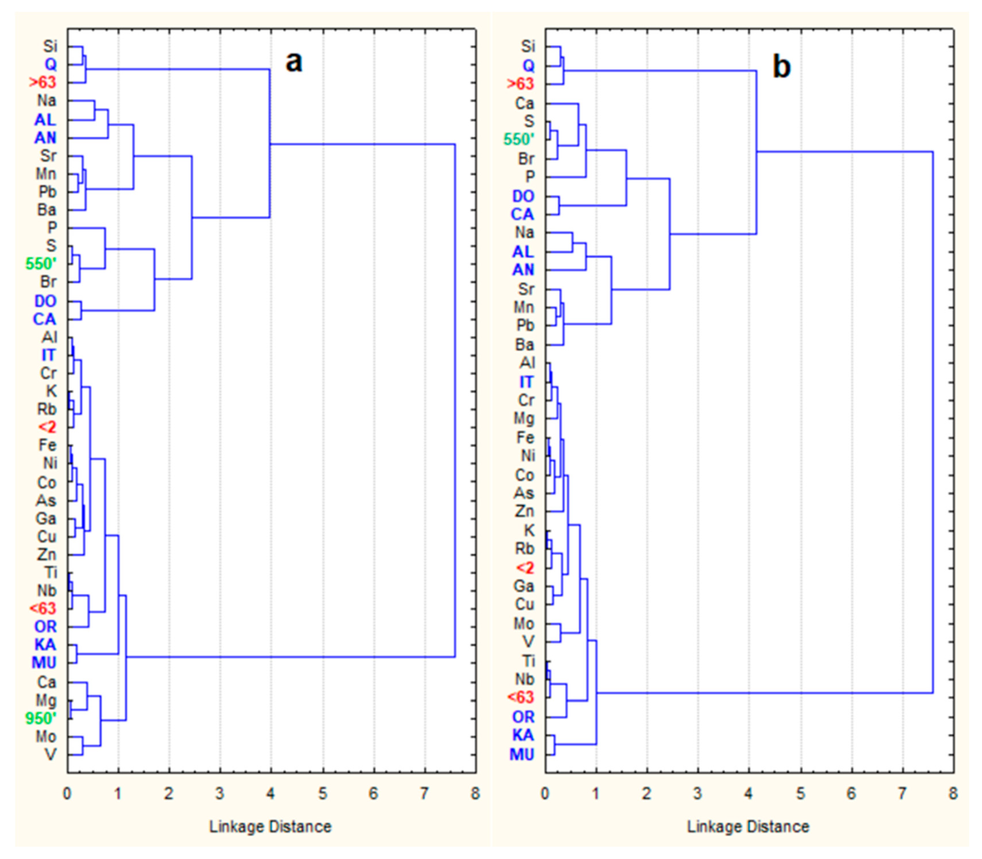
• This research has revealed the following eight influential non-elemental variables that are significantly (p < 0.01) correlated with all ten studied PHEs: (i) clay (<2 μm), sand (>63 μm), and fine (<63 μm) fractions; (ii) illite, kaolinite, orthoclase, and quartz with significant loadings on the most variable mineralogical factor; and (iii) LOI at 950 °C (950′). Partly influential non-elemental variables included (i) muscovite related to the same factor and significantly correlated with eight PHEs, i.e., As, Ba, Co, Cr, Cu, Ni, V, and Zn; (ii) a silt fraction (2–63 μm) significantly correlated with nine PHEs, i.e., As, Ba, Co, Cr, Cu, Mo, Ni, Pb, and Zn; and (iii) LOI at 550 °C (550′) significantly correlated with four PHEs, i.e., As, Cr, Pb, and Zn. Dolomite, calcite, albite, and anorthite had either an insignificant influence on the PHEs or were correlated with only one or two of them. The group of influential non-elemental variables was adjusted, excluding LOI at 950 °C due to its insignificant correlation with calcite and lower correlation with dolomite than with the most variable mineral group. Presumably nonharmful chemical elements significantly correlated with all influential non-elemental variables were Al, Ga, Fe, K, Nb, Rb, Si, Ti, and Mg. The first eight elements were attributed to potential reference elements (PREs) but not Mg due to its ambiguous clusters in two dendrograms of basic variables: (i) Ca–Mg–950′ when the 950′ variable was included and (ii) Al–illite–Cr–Mg when this variable was omitted.
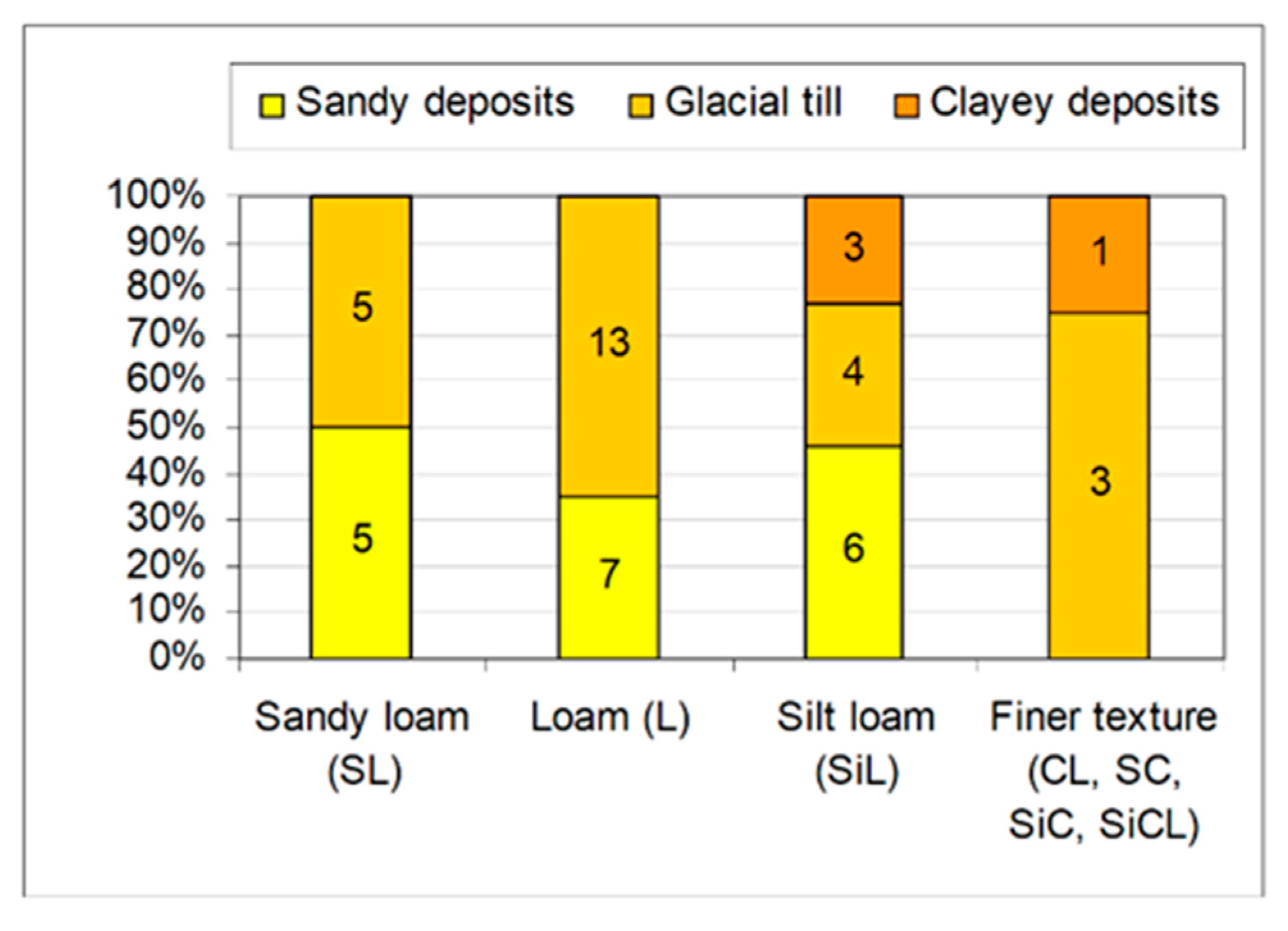
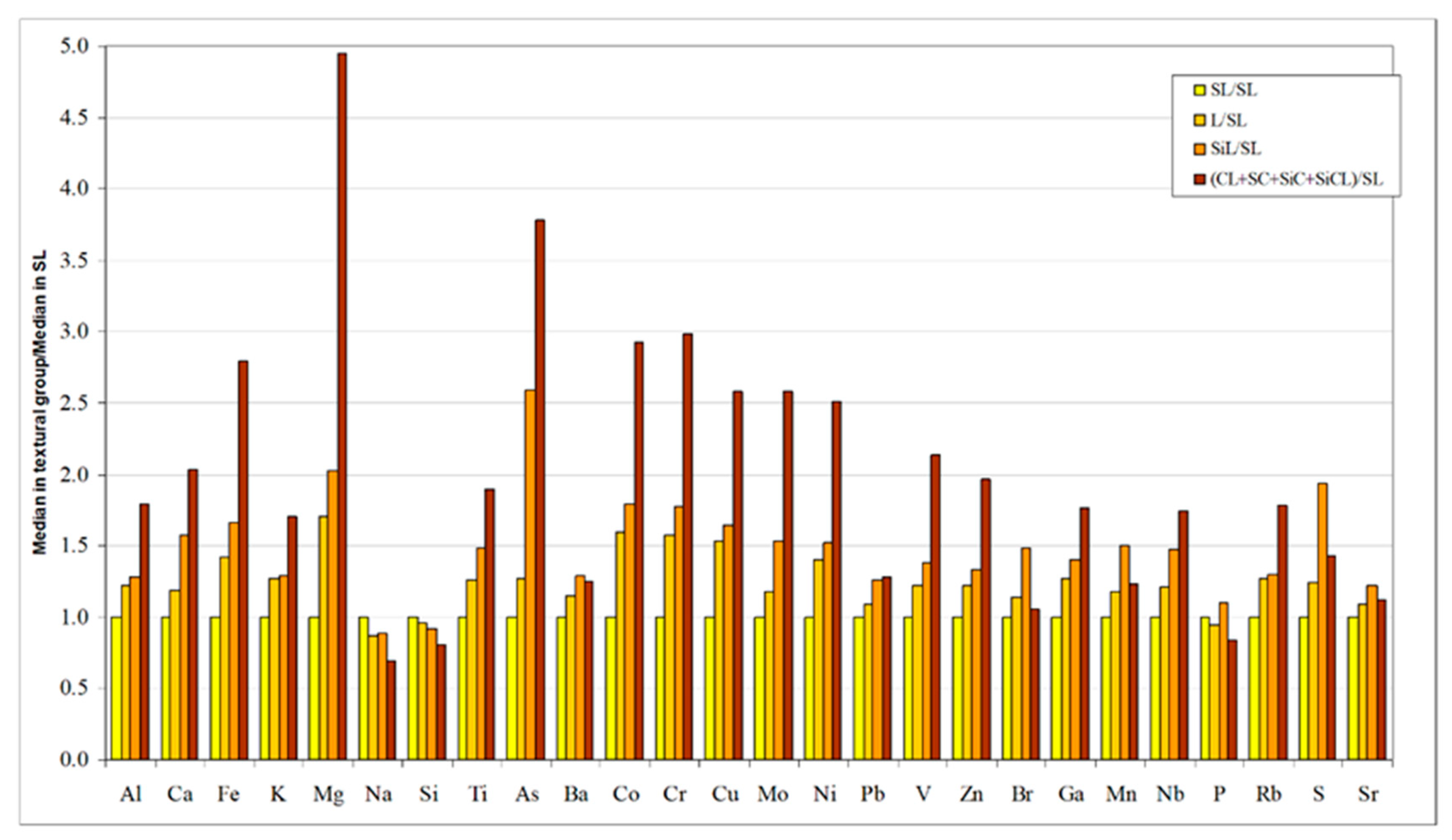
• Lithology is the key property of Quaternary deposits that influences the values of 34 out of the 41 tested variables, as evident from the comparison of groups of sites on sandy deposits, glacial till, and clayey deposits. Statistically significant (p < 0.05) differences among groups were found for (i) four grain size fractions, namely clay, silt, sand, and the fine fraction; (ii) six minerals, namely illite, kaolinite, orthoclase, quartz, albite, and dolomite; (iii) LOI at 550 °C, which is an indicator of organic matter; and (iv) the contents of nine PHEs, namely As, Ba, Co, Cr, Cu, Ni, Pb, V, and Zn, and all eight PREs, namely Al, Ga, Fe, K, Nb, Rb, Si, and Ti, as well as Ca, Sr, Mn, Br, and S. This indicates that Quaternary lithology is reflected in all influential non-elemental variables, all PREs, and almost all PHEs in the topsoil. The results of multiple comparisons among the aforementioned groups, as well as the prevalence of sandy Quaternary deposits in Vilnius City, suggest that, for a substantiated estimation of the geochemical indices of PHEs, the background subset (BS) selected from peri-urban sites should have relatively lower contents of PHEs and many possibly nonharmful chemical elements compared to the sites attributed to the non-background subset (NBS).
• The dendrogram of sites, compiled using 40 basic variables—26 elements, including As, Ba, Co, Cr, Cu, Mo, Ni, Pb, V, and Zn (ten PHEs); Al, Fe, Ga, K, Nb, Rb, Si, and Ti (eight PREs); Ca, Mg, Na, Br, Mn, P, S, and Sr (eight presumably nonharmful elements); <2 µm, <63 µm, and >63 µm grain size fractions; LOI at 550 °C and LOI at 950 °C; and also illite, kaolinite, muscovite, orthoclase, quartz, dolomite, calcite, albite, and anorthite (nine common minerals)—demonstrates that topsoil texture classes are much better reflected in clusters than lithological groups of Quaternary deposits. The increase in the median contents of PHEs and a greater portion of presumably nonharmful elements towards finer topsoil texture shows that the percentage of sandy loam and loam in each cluster can be a useful criterion when selecting clusters for inclusion in BS.
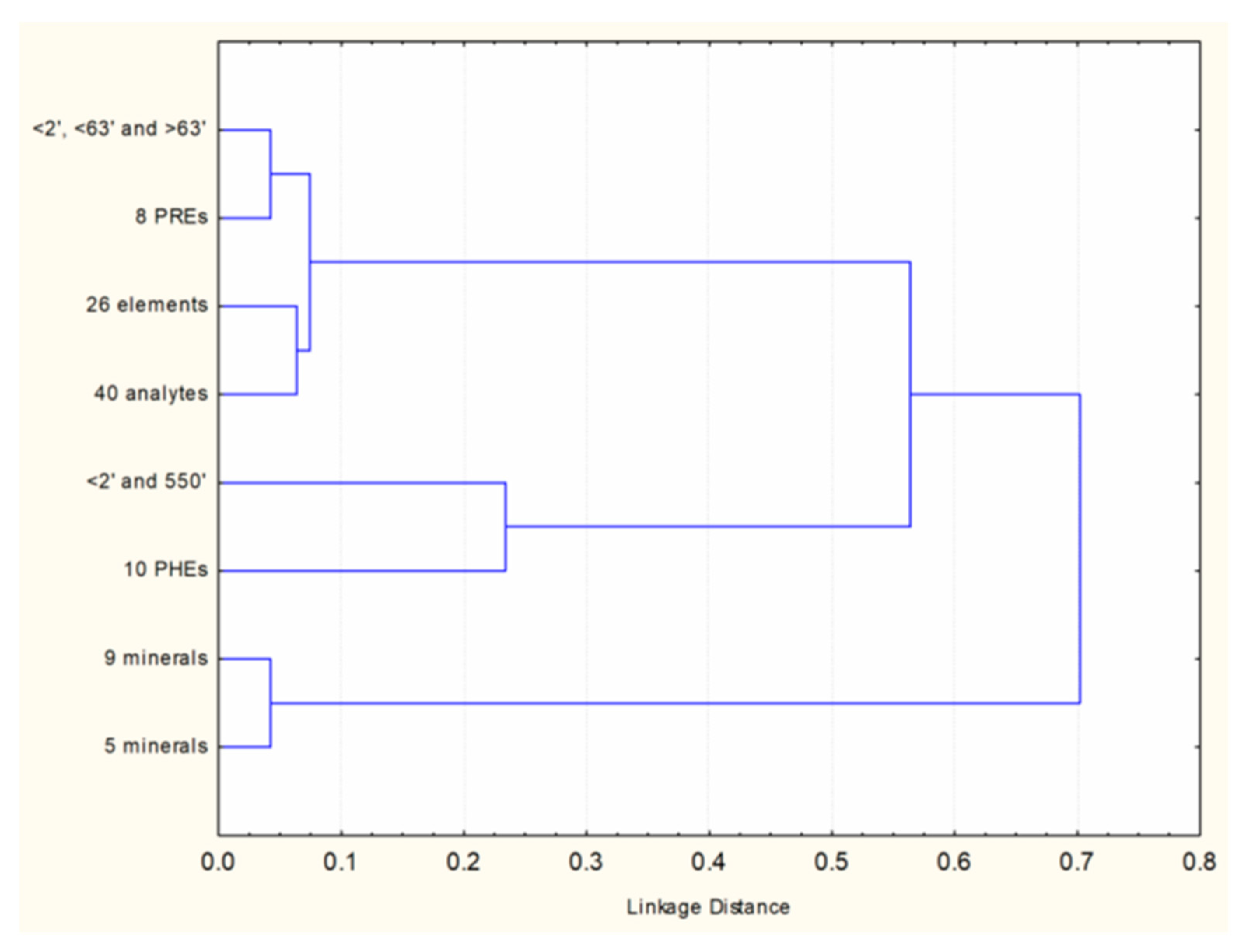
• The ranking of eight statistical site classifications into BS and NBS, using cluster analysis of the selected variables, was based on generalized indices of elemental contrast ratios—the median in the subset with relatively higher values divided by the median in the subset with relatively lower values. The dendrogram of these eight versions revealed an associated group of four high-ranked site classifications: (i) using the aforementioned 40 basic variables; (ii) using the aforementioned 26 elements, i.e., ten PHEs, eight PREs, and eight presumably nonharmful elements; (iii) using <2 µm, <63 µm, and >63 µm grain size fractions; and (iv) using PREs Al, Fe, Ga, K, Nb, Rb, Si, and Ti. Multiple comparisons did not reveal statistically significant (p < 0.05) differences in the elemental contents between the refined background subsets based on these four site classifications, so the respective BVs were very similar. The last two versions, based on either a few elements or a few non-elemental variables, are less expensive and are recommended for the selection of BS. The fractions 2 μm, <63 μm, and >63 μm, as well as PREs Al, Fe, Ga, K, Nb, Rb, Si, and Ti, can be recommended as reference variables. Meanwhile, the less-associated group of four low-ranked site classifications—two of which are based on mineralogical variables, one on the contents of PHEs, and one on <2 μm and LOI at 550 °C variables—are less effective for the selection of BS, especially the last version. This result provides a BS where the contents of K, Ba, Co, Cu, Ga, and Rb statistically differ from some other versions of background subsets, and the respective BVs are higher.
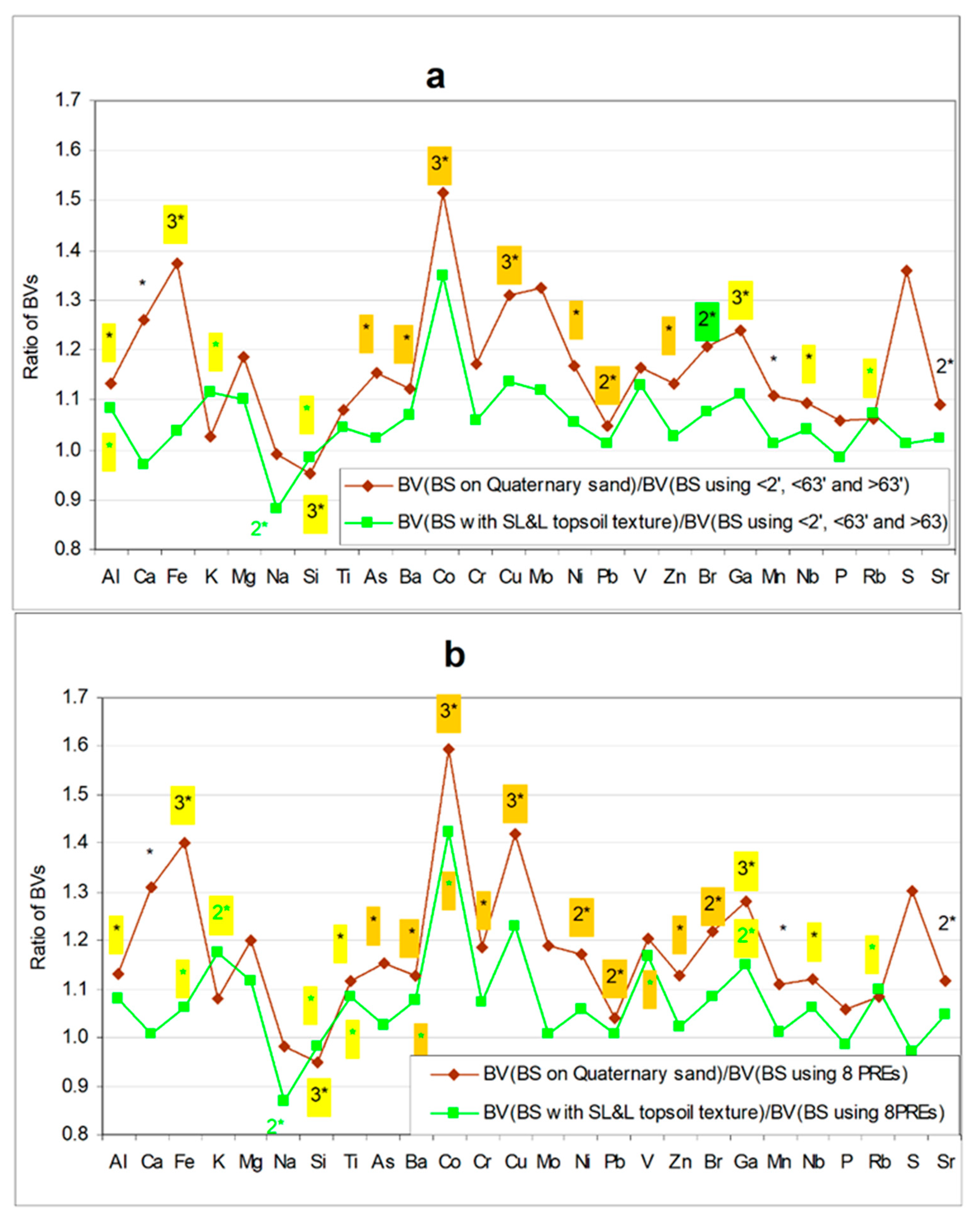
• The advantage of statistical site classification based on clusters distinguished using the <2 µm, <63 µm, and >63 µm fractions determined in topsoil in comparison with nonstatistical site classifications based on Quaternary deposits or topsoil texture classes is confirmed by the higher elemental contrast ratios and more significant differences between BS and NBS. Both statistical site classifications based on reference variables <2 µm, <63 µm, and >63 µm or Al, Fe, Ga, K, Nb, Rb, Si, and Ti ensure higher BVs of Si and lower BVs of the other PREs, as well as PHEs and potentially useful elements S and Br, which are related to the partly influential indicator of organic matter (LOI at 550 °C). Therefore, the substantiation of these BVs seems to be adequate.

References

1. Nag, R.; O’Rourke, S.M.; Cummins, E. Risk factors and assessment strategies for the evaluation of human or environmental risk from metal(loid)s—A focus on Ireland. Sci. Total Environ. 2022, 802, 149839. [Google Scholar] [CrossRef] [PubMed]
2. Massas, I.; Ehaliotis, C.; Kalivas, D.; Panagopoulou, G. Concentrations and availability indicators of soil heavy metals; the case of children’s playgrounds in the City of Athens (Greece). Water Air Soil Pollut. 2010, 212, 51–63. [Google Scholar] [CrossRef]
3. Taraškevičius, R.; Zinkutė, R.; Gedminienė, L.; Stankevičius, Ž. Hair geochemical composition of children from Vilnius kindergartens as an indicator of environmental conditions. Environ. Geochem. Health 2018, 40, 1817–1840. [Google Scholar] [CrossRef] [PubMed]
4. Zhang, Y.; Dong, J.; Li, X.; Liu, B.; Wang, J.; Cao, Y.; Li, T. Comprehensive investigation of multi-trace metals/metalloids in urban soil and street dust within Xi’an ancient city wall (NW, China). Environ. Earth Sci. 2021, 80, 587. [Google Scholar] [CrossRef]
5. Kolawole, T.O.; Olatunji, A.S.; Jimoh, M.T.; Fajemila, O.T. Heavy metal contamination and ecological risk assessment in soils and sediments of an industrial area in Southwestern Nigeria. J. Health Pollut. 2018, 8, 180906. [Google Scholar] [CrossRef]
6. Carlon, C.; D’Alessandro, M.; Swartjes, F. Derivation Methods of Soil Screening Values in Europe: A Review and Evaluation of National Procedures towards Harmonization; EUR 22805-EN; Carlon, C., Ed.; European Commission, Joint Research Centre: Ispra, Italy, 2007; 306p, ISBN 978-92-79-05238-5. ISSN 1018-5593. Available online: https://esdac.jrc.ec.europa.eu/ESDB_Archive/eusoils_docs/other/EUR22805.pdf (accessed on 25 January 2022).
7. Swartjes, F.A. Risk-based assessment of soil and groundwater quality in the Netherlands: Standards and remediation urgency. Risk Anal. 1999, 19, 1235–1249. [Google Scholar] [CrossRef] [PubMed]
8. Albanese, S.; Cicchella, D.; Lima, A.; De Vivo, B. Geochemical mapping of urban areas. In Environmental Geochemistry: Site Characterization, Data Analysis and Case Histories, 2nd ed.; De Vivo, B., Belkin, H.E., Lima, A., Eds.; Elsevier: Amsterdam, The Netherlands, 2018; pp. 133–151. ISBN 978-0-444-63763-5. [Google Scholar] [CrossRef]
9. Díaz Rizo, O.; Fonticiella Morell, D.; Arado Lopez, J.O.; Borrell Munoz, J.L.; D’Alessandro Rodriguez, K.; Lopez Pino, N. Spatial distribution and contamination assessment of heavy metals in urban topsoils from Las Tunas City, Cuba. Bull. Environ. Contam. Toxicol. 2013, 91, 29–35. [Google Scholar] [CrossRef]
10. Tahmasbian, I.; Nasrazadani, A.; Shoja, H.; Sinegani, S.; Akbar, A. The effects of human activities and different land-use on trace element pollution in urban topsoil of Isfahan (Iran). Environ. Earth Sci. 2014, 71, 1551–1560. [Google Scholar] [CrossRef]
11. Labaz, B.; Kabala, C.; Waroszewski, J. Ambient geochemical baselines for trace elements in Chernozems—Approximation of geochemical soil transformation in an agricultural area. Environ. Monit. Assess. 2019, 191, 19. [Google Scholar] [CrossRef]
12. Zhang, H.; Yu, M.; Xu, H.; Wen, H.; Fan, H.; Wang, T.; Liu, J. Geochemical baseline determination and contamination of heavy metals in the urban topsoil of Fuxin City, China. J. Arid Land 2020, 12, 1001–1017. [Google Scholar] [CrossRef]
13. Dung, T.T.T.; Cappuyns, V.; Swennen, R.; Phung, N.K. From geochemical background determination to pollution assessment of heavy metals in sediments and soils. Rev. Environ. Sci. Biotechnol. 2013, 12, 335–353. [Google Scholar] [CrossRef]
14. Lee, C.S.; Li, X.D.; Shi, W.Z.; Cheung, S.C.; Thornton, I. Metal contamination in urban, suburban and country park soils of Hong Kong: A study based on GIS and multivariate statistics. Sci. Total Environ. 2006, 356, 45–61. [Google Scholar] [CrossRef]
15. Struijs, J.; van de Meent, D.; Peijnenburg, W.J.G.M.; van den Hoop, M.A.G.T.; Crommentuijn, T. Added risk approach to derive maximum permissible concentrations for heavy metals: How to take natural background levels into account. Ecotox. Environ. Saf. 1997, 37, 112–118. [Google Scholar] [CrossRef] [PubMed]
16. Crommentuijn, T.; Sijm, D.; de Bruijn, J.; van den Hoop, M.; van Leeuwen, K.; van de Plassche, E. Maximum permissible and negligible concentrations for metals and metalloids in the Netherlands, taking into account background concentrations. J. Environ. Manag. 2000, 60, 121–143. [Google Scholar] [CrossRef]
17. Gałuszka, A. A review of geochemical background concepts and an example using data from Poland. Environ. Geol. 2007, 52, 861–870. [Google Scholar] [CrossRef]
18. Kara, M.; Dumanoğlu, Y.; Altıok, H.; Elbir, T.; Odabasi, M.; Bayram, A. Spatial distribution and source identification of trace elements in topsoil from heavily industrialized region, Aliaga, Turkey. Environ. Monit. Assess. 2014, 186, 6017–6038. [Google Scholar] [CrossRef]
19. Bityukova, L.; Shogenova, A.; Birke, M. Urban geochemistry: A study of element distributions in the soils of Tallinn (Estonia). Environ. Geochem. Health 2000, 22, 173–193. [Google Scholar] [CrossRef]
20. Yay, O.D.; Alagha, O.; Tuncel, G. Multivariate statistics to investigate metal contamination in surface soil. J. Environ. Manag. 2008, 86, 581–594. [Google Scholar] [CrossRef]
21. Wang, X.S.; Qin, Y.; Sang, S.X. Accumulation and sources of heavy metals in urban topsoils: A case study from the city of Xuzhou, China. Environ. Geol. 2005, 48, 101–107. [Google Scholar] [CrossRef]
22. Gong, M.; Wu, L.; Bi, X.; Ren, L.; Wang, L.; Ma, Z.; Bao, Z.; Li, Z. Assessing heavy-metal contamination and sources by GIS-based approach and multivariate analysis of urban–rural topsoils in Wuhan, central China. Environ. Geochem. Health 2010, 32, 59–72. [Google Scholar] [CrossRef]
23. Zhang, C. Using multivariate analyses and GIS to identify pollutants and their spatial patterns in urban soils in Galway, Ireland. Environ. Pollut. 2006, 142, 501–511. [Google Scholar] [CrossRef]
24. Zhang, X.P.; Deng, W.; Yang, X.M. The background concentrations of 13 soil trace elements and their relationship to parent materials and vegetation in Xizang (Tibet), China. J. Asian Earth Sci. 2002, 21, 167–174. [Google Scholar] [CrossRef]
25. Díaz Rizo, O.; Coto Hernández, I.; Arado López, J.O.; Díaz Arado, O.; López Pino, N.; D′Alessandro Rodríguez, K. Chromium, cobalt and nickel contents in urban soils of Moa, Northeastern Cuba. Bull. Environ. Contam. Toxicol. 2011, 86, 189–193. [Google Scholar] [CrossRef] [PubMed]
26. Reimann, C.; de Caritat, P. Distinguishing between natural and anthropogenic sources for elements in the environment: Regional geochemical surveys versus enrichment factors. Sci. Total Environ. 2005, 337, 91–107. [Google Scholar] [CrossRef] [PubMed]
27. Chen, J.; Wei, F.; Zheng, C.; Wu, Y.; Adriano, D.C. Background concentrations of elements in soils of China. Water Air Soil Pollut. 1991, 57, 699–712. [Google Scholar] [CrossRef]
28. Gosar, M.; Šajn, R.; Bavec, Š.; Gaberšek, M.; Pezdir, V.; Miler, M. Geochemical background and threshold for 47 chemical elements in Slovenian topsoil. Geologija 2019, 62, 5–57. [Google Scholar] [CrossRef]
29. Reimann, C.; Garrett, R. Geochemical background—Concept and reality. Sci. Total Environ. 2005, 350, 12–27. [Google Scholar] [CrossRef] [PubMed]
30. Yang, Z.; Lu, W.; Long, Y.; Bao, X.; Yang, Q. Assessment of heavy metals contamination in urban topsoil from Changchun City, China. J. Geochem. Explor. 2011, 108, 27–38. [Google Scholar] [CrossRef]
31. Zhang, M.; Li, X.; Yang, R.; Wang, J.; Ai, Y.; Gao, Y.; Zhang, Y.; Zhang, X.; Yan, X.; Liu, B.; et al. Multipotential toxic metals accumulated in urban soil and street dust from Xining City, NW China: Spatial occurrences, sources, and health risks. Arch. Environ. Contam. Tox. 2019, 76, 308–330. [Google Scholar] [CrossRef]
32. Díaz Rizo, O.; Echeverría Castillo, F.; Arado López, J.O.; Hernández Merlo, M. Assessment of heavy metal pollution in urban soils of Havana City, Cuba. Bull. Environ. Contam. Toxicol. 2011, 87, 414–419. [Google Scholar] [CrossRef]
33. Zinkutė, R.; Taraškevičius, R.; Jankauskaitė, M.; Stankevičius, Ž. Methodological alternatives for calculation of enrichment factors used for assessment of topsoil contamination. J. Soil Sediment. 2017, 17, 440–452. [Google Scholar] [CrossRef]
34. Lu, W.; Liu, J.; Wang, Y.; Zhang, N.; Ren, L.; Bao, L. Cumulative risk assessment of soil-crop potentially toxic elements accumulation under two distinct pollution systems. Minerals 2022, 12, 1134. [Google Scholar] [CrossRef]
35. Matschullat, J.; Ottenstein, R.; Reimann, C. Geochemical background—Can we calculate it? Environ. Geol. 2000, 39, 990–1000. [Google Scholar] [CrossRef]
36. Reimann, C.; Filzmoser, P.; Garrett, R.G. Background and threshold: Critical comparison of methods of determination. Sci. Total Environ. 2005, 346, 1–16. [Google Scholar] [CrossRef] [PubMed]
37. Chen, T.B.; Zheng, Y.-M.; Lei, M.; Huang, Z.-C.; Wu, H.-T.; Chen, H.; Fan, K.-K.; Yu, K.; Wu, X.; Tian, Q.-Z. Assessment of heavy metal pollution in surface soils of urban parks in Beijing, China. Chemosphere 2005, 60, 542–551. [Google Scholar] [CrossRef]
38. Tack, F.M.G.; Verloo, M.G.; Vanmechelen, L.; van Ranst, E. Baseline concentration levels of trace elements as a function of clay and organic carbon contents in soils in Flanders (Belgium). Sci. Total Environ. 1997, 201, 113–123. [Google Scholar] [CrossRef]
39. Delbecque, N.; van Ranst, E.; Dondeyne, S.; Mouazen, A.M.; Vermeir, P.; Verdoodt, A. Geochemical fingerprinting and magnetic susceptibility to unravel the heterogeneous composition of urban soils. Sci. Total Environ. 2022, 847, 157502. [Google Scholar] [CrossRef] [PubMed]
40. Zinkutė, R.; Taraškevičius, R.; Jankauskaitė, M.; Kazakauskas, V.; Stankevičius, Ž. Influence of site-classification approach on geochemical background values. Open Chem. 2020, 18, 1391–1411. [Google Scholar] [CrossRef]
41. Wang, X.-S.; Qin, Y. Some characteristics of the distribution of heavy metals in urban topsoil of Xuzhou, China. Environ. Geochem. Health 2007, 29, 11–19. [Google Scholar] [CrossRef]
42. Rothwell, K.A.; Cooke, M.P. A comparison of methods used to calculate normal background concentrations of potentially toxic elements for urban soil. Sci. Total Environ. 2015, 532, 625–634. [Google Scholar] [CrossRef]
43. Zinkutė, R.; Taraškevičius, R.; Gulbinskas, S.; Stankevičius, Ž.; Jankauskaitė, M. Variability of estimated contamination extent depending on calculation methods. In Environment. Technology. Resources, Proceedings of the 10th International Scientific and Practical Conference, Rezekne, Latvia, 18–20 June 2015; Rezeknes Augstskola: Rezekne, Latvia, 2015; Volume II, pp. 337–343. [Google Scholar] [CrossRef]
44. Zhao, F.J.; McGrath, S.P.; Merrington, G. Estimates of ambient background concentrations of trace metals in soils for risk assessment. Environ. Pollut. 2007, 148, 221–229. [Google Scholar] [CrossRef] [PubMed]
45. Salonen, V.-P.; Korkka-Niemi, K. Influence of parent sediments on the concentration of heavy metals in urban and suburban soils in Turku, Finland. Appl. Geochem. 2007, 22, 906–918. [Google Scholar] [CrossRef]
46. Baltrūnas, V.; Karmaza, B.; Pukelytė, V.; Karmazienė, D. Pleistocene architecture and stratigraphy in the contact zone of ice streams and lobes in the south-eastern part of the Baltic Region. Quat. Int. 2019, 501, 21–32. [Google Scholar] [CrossRef]
47. World Reference Base for Soil Resources 2014. International Soil Classification System for Naming Soils and Creating Legends for Soil Maps; Update 2015. World Soil Resources Reports 106; FAO: Rome, Italy, 2015; Available online: http://www.fao.org/3/i3794en/I3794en.pdf (accessed on 20 April 2019).
48. Santisteban, J.I.; Mediavilla, R.; López-Pamo, E.; Dabrio, C.J.; Ruiz-Zapata, M.B.; Garcia, M.J.G.; Castano, S.; Martinez-Alfaro, P.E. Loss on ignition: A qualitative or quantitative method for organic matter and carbonate mineral content in sediments? J. Paleolim. 2004, 32, 287–299. [Google Scholar] [CrossRef]
49. Prohić, E.; Miko, S.; Peh, Z. Normalisation and trace element contamination of soils in a Karstic Polje—An example from the Sinjsko Polje, Croatia. Geol. Croat. 1995, 48, 67–86. Available online: http://www.geologiacroatica.hr/index.php/GC/article/view/GC.1995.06 (accessed on 20 May 2019).
50. Kvartero Geologinis Žemėlapis M 1:200,000 (in Lithuanian). Available online: https://www.lgt.lt/epaslaugos/elpaslauga.xhtml (accessed on 10 January 2022).
51. Schramm, R.; Heckel, J. Fast analysis of traces and major elements with ED(P)XRF using polarized Xrays: TURBOQUANT. J Phys. IV 1998, 8, Pr5-335–Pr5-342. [Google Scholar] [CrossRef]
52. SPECTRO XEPOS. ED-XRF Spectrometers. Introducing a New Era in Analytical Performance. Available online: www.spectro.com/-/media/ametekspectro/documents/brochure/spectro_xepos_en.pdf (accessed on 9 November 2023).
53. Analyzing Trace Elements in Pressed Pellets of Geological Materials Using ED-XRF. Available online: https://extranet.spectro.com/-/media/5C512E72-682D-45D8-AE56-6740529341BC.pdf (accessed on 19 November 2023).
54. MCERTS Standard for Laboratories Undertaking Chemical Testing of Soil. LIT 6625. Environmental Agency, October 2023. Available online: https://assets.publishing.service.gov.uk/media/654a396ee2e16a000d42aaec/LIT_6625_-_MCERTS_-_performance_standard_for_laboratories_undertaking_chemical_testing_of_soil.pdf (accessed on 9 November 2023).
55. International Soil-Analytical Exchange Programme—ISE. Proficiency Tests. Available online: https://www.wepal.nl/en/wepal/home/proficiency-tests/soil/ise.htm (accessed on 9 November 2023).
56. Jurgelėnė, Ž.; Montvydienė, D.; Stakėnas, S.; Poviliūnas, J.; Račkauskas, S.; Taraškevičius, R.; Skrodenytė-Arbačiauskienė, V.; Kazlauskienė, N. Impact evaluation of marking Salmo trutta with Alizarin Red S produced by different manufacturers. Aquat. Toxicol. 2022, 242, 106051. [Google Scholar] [CrossRef]
57. Taraškevičius, R.; Motiejūnaitė, J.; Zinkutė, R.; Eigminienė, A.; Gedminienė, L.; Stankevičius, Ž. Similarities and differences in geochemical distribution patterns in epiphytic lichens and topsoils from kindergarten grounds in Vilnius. J. Geochem. Explor. 2017, 183, 152–165. [Google Scholar] [CrossRef]
58. Matulevičiūtė, D.; Motiejūnaitė, J.; Uogintas, D.; Taraškevičius, R.; Dagys, M.; Rašomavičius, V. Decline of a protected coastal pine forest under impact of a colony of great cormorants and the rate of vegetation change under ornithogenic influence. Silva fenica 2018, 52, 7699. [Google Scholar] [CrossRef]
59. Taraškevičius, R.; Kazakauskas, V.; Sarcevičius, S.; Zinkutė, R.; Suzdalev, S. Case study of geochemical clustering as a tool for tracing sources of clays for archaeological and modern bricks. Baltica 2019, 32, 139–155. [Google Scholar] [CrossRef]
60. Rapalis, P.; Zinkutė, R.; Lazareva, N.; Suzdalev, S.; Taraškevičius, R. Geochemistry of the dust collected by passive samplers as a tool for search of pollution sources: The case of Klaipėda Port, Lithuania. Appl. Sci. 2021, 11, 11157. [Google Scholar] [CrossRef]
61. Šatavičė, E.; Skridlaitė, G.; Grigoravičiūtė-Puronienė, I.; Kareiva, A.; Selskienė, A.; Suzdalev, S.; Žaludienė, G.; Taraškevičius, R. Corded ware and contemporary hunter-gatherer pottery from Southeast Lithuania: Technological insights through geochemical and mineralogical approaches. Minerals 2022, 12, 1006. [Google Scholar] [CrossRef]
62. Šinkovičová, M.; Igaz, D.; Kondrlová, E.; Jarošová, M. Soil particle size analysis by laser diffractometry: Result comparison with pipette method. IOP Conf. Ser. Mater. Sci. Eng. 2017, 245, 072025. [Google Scholar] [CrossRef]
63. Bengtsson, L.; Enell, M. Chemical analysis. In Handbook of Holocene Palaeoecology and Palaeohydrology; Begrlund, B.E., Ed.; John Wiley & Sons: Chichester, UK, 1986; pp. 423–454. ISBN 0471 00691 3. [Google Scholar]
64. StatSoft, Inc. STATISTICA (Data Analysis Software System), Version 8.0. 2007. Available online: https://www.statsoft.com (accessed on 19 November 2023).
65. Microsoft, Inc. Microsoft Office Excel; Microsoft, Inc.: Redmond, WA, USA, 2003. [Google Scholar]
66. Microsoft 365, Inc. Excel in Microsoft 365. Available online: https://www.microsoft365.com/ (accessed on 10 September 2023).
67. Eberl, D.D.; Smith, D.B. Mineralogy of soils from two continental-scale transects across the United States and Canada and its relation to soil geochemistry and climate. Appl. Geochem. 2009, 24, 1394–1404. [Google Scholar] [CrossRef]
68. Drew, L.J.; Grunsky, E.C.; Sutphin, D.M.; Laurel, G.; Woodruff, L.G. Multivariate analysis of the geochemistry and mineralogy of soils along two continental-scale transects in North America. Sci. Total Environ. 2010, 409, 218–227. [Google Scholar] [CrossRef] [PubMed]
69. Kumari, N.; Mohan, C. Basics of clay minerals and their characteristic properties. In Clay and Clay Minerals; Do Nascimento, G.M., Ed.; IntechOpen: London, UK, 2021; pp. 1–29. ISBN 978-1-83969-565-0. [Google Scholar] [CrossRef]
70. Garcia-Gonzalez, M.T.; Aragonezes, F.J. Relationship between mineralogy and elemental composition in strongly developed soils using principal component analysis. Aust. J. Soil Res. 1992, 30, 395–408. Available online: http://hdl.handle.net/10261/24827 (accessed on 15 November 2022). [CrossRef]
71. Van der Veer, G. Geochemical soil survey of the Netherlands: Atlas of major and trace elements in topsoil and parent material; assessment of natural and anthropogenic enrichment factors. Neth. Geogr. Stud. 2006, 347, 1–245. Available online: https://dspace.library.uu.nl (accessed on 11 June 2023).
72. Blum, A.E. Felspars in weathering. In Feldspars and Their Reactions; Parsons, I., Ed.; Kluwer Academic Publishers: Dordrecht, The Netherlands, 1994; pp. 595–630. ISBN 0 7923 2722 5. [Google Scholar]
73. Dean, W.E., Jr. Determination of carbonate and organic matter in calcareous sediments and sedimentary rocks by loss on ignition: Comparison with other methods. J. Sed. Petrol. 1974, 44, 242–248. [Google Scholar] [CrossRef]
74. Heiri, O.; Lotter, A.F.; Lemcke, G. 2001. Loss on ignition as a method for estimating organic and carbonate content in sediments: Reproducibility and comparability of results. J. Paleolim. 2001, 25, 101–110. [Google Scholar] [CrossRef]
75. Gedminienė, L.; Šiliauskas, L.; Skuratovič, Ž.; Taraškevičius, R.; Zinkutė, R.; Kazbaris, M.; Ežerinskis, Ž.; Šapolaitė, J.; Gastevičienė, N.; Šeirienė, V.; et al. The Lateglacial-Early Holocene dynamics of the sedimentation environment based on the multi-proxy abiotic study of Lieporiai palaeolake, Northern Lithuania. Baltica 2019, 32, 63–77. [Google Scholar] [CrossRef]
76. De Vos, B.; Vandecasteele, B.; Deckers, J.; Muys, B. Capability of loss-on-ignition as a predictor of total organic carbon in non-calcareous forest soils. Commun. Soil Sci. Plan. 2005, 36, 2899–2921. [Google Scholar] [CrossRef]
77. De Vos, B.; Lettens, S.; Muys, B.; Deckers, J.A. Walkley-Black analysis of forest soil organic carbon: Recovery, limitations and uncertainty. Soil Use Manag. 2007, 23, 221–229. [Google Scholar] [CrossRef]
78. Kabata-Pendias, A.; Pendias, H. Trace Elements in Soils and Plants, 3rd ed.; CRC Press LCC: Washington, DC, USA, 2001; pp. 51–57+64–71. ISBN 0-8493-1575-1. [Google Scholar]
79. He, G.; Zhang, Z.; Wu, X.; Cui, M.; Zhang, J.; Huang, X. Adsorption of heavy metals on soil collected from Lixisol of typical karst areas in the presence of CaCO3 and soil clay and their competition behavior. Sustainability 2020, 12, 7315. [Google Scholar] [CrossRef]
80. Wang, J.P.; Wang, X.J.; Zhang, J. Evaluating loss-on-ignition method for determinations of soil organic and inorganic carbon in arid soils of northwestern China. Pedosphere 2013, 23, 593–599. [Google Scholar] [CrossRef]
81. De Araújo, J.H.; da Silva, N.F.; Acchar, W.; Gomes, U.U. Thermal Decomposition of Illite. Mater. Res. 2004, 7, 359–361. [Google Scholar] [CrossRef]
82. Sparks, D.L. Chemistry of soil organic matter. In Environmental Soil Chemistry, 2nd ed.; Academic Press, Elsevier Science: San Diego, CA, USA, 2003; pp. 75–113. ISBN 9780080494807. [Google Scholar] [CrossRef]
83. Szymański, W.; Siwek, J.; Skiba, M.; Wojtuń, B.; Samecka-Cymerman, A.; Pech, P.; Polechońska, L.; Smyrak-Sikora, A. Properties and mineralogy of topsoil in the town of Longyearbyen (Spitsbergen, Norway). Polar Rec. 2019, 55, 102–114. [Google Scholar] [CrossRef]
84. Covelo, E.F.; Vega, F.A.; Andrade, M.L. Competitive sorption and desorption of heavy metals by individual soil components. J. Hazard. Mater. 2007, 140, 308–315. [Google Scholar] [CrossRef]
85. Van den Hoop, M.A.G.T. Metal Speciation in Dutch Soils: Field-Based Partition Coefficients for Heavy Metals at Background Levels. Rijksinstituut voor Volksgesondheid en Milieu bildhoven. Rapport Nr. 719101013. 1995. Available online: https://www.rivm.nl/bibliotheek/rapporten/719101013.pdf (accessed on 15 December 2022).
86. Spijker, J. The Dutch Soil Type Correction. An Alternative Approach. RIVM Report 607711005. National Institute for Public Health and the Environment. Ministry of Health, Welfare and Sport. 2012. Available online: https://www.rivm.nl/bibliotheek/rapporten/607711005.pdf (accessed on 10 October 2022).
87. Appleton, J.D.; Johnson, C.C.; Ander, E.L.; Flight, D.M.A. Geogenic signatures detectable in topsoils of urban and rural domains in the London region, UK, using parent material classified data. Appl. Geochem. 2013, 39, 169–180. [Google Scholar] [CrossRef]
88. Phosphorus Basics: Understanding Phosphorus forms and Their Cycling in the Soil. Agriculture Extension. Alabama A&M and Auburn Universities. ANR-2535. Available online: https://www.aces.edu/wp-content/uploads/2019/04/ANR-2535-Phosphorus-Basics_041719L.pdf (accessed on 21 July 2022).
89. Rawlins, B.G.; Webster, R.; Lister, T.R. The influence of parent material on topsoil geochemistry in Eastern England. Earth Surf. Process. 2003, 28, 1389–1409. [Google Scholar] [CrossRef]
90. Norra, S.; Lanka-Panditha, M.; Kramar, U.; Stüben, D. Mineralogical and geochemical patterns of urban surface soils, the example of Pforzheim, Germany. Appl. Geochem. 2006, 21, 2064–2081. [Google Scholar] [CrossRef]
91. Bityukova, L.; Birke, M. Urban geochemistry of Tallinn (Estonia): Major and trace-elements distribution in topsoil. In Mapping the Chemical Environment of Urban Areas; Johnson, C.C., Demetriades, A., Locutura, J., Ottesen, R.T., Eds.; Wiley: Chichester, UK, 2011; pp. 348–363. ISBN 978-0-470-67007-1. [Google Scholar] [CrossRef]
92. Dantu, S. Spatial distribution and geochemical baselines of major/trace elements in soils of Medak district, Andhra Pradesh, India. Environ. Earth Sci. 2014, 72, 955–981. [Google Scholar] [CrossRef]
93. Plant, J.A.; Whittaker, A.; Demetriades, A.; De Vivo, B.; Lexa, J. The geological and tectonic framework of Europe. In Geochemical Atlas of Europe. Part 1: Background Information, Methodology and Maps; Salminen, R., Ed.; Geological Survey of Finland: Espoo, Finland, 2005; ISBN 951-690-013-2. Available online: http://weppi.gtk.fi/publ/foregsatlas/article.php?id=4 (accessed on 21 October 2022).
94. Guobytė, R.; Satkūnas, J. Pleistocene glaciations in Lithuania. In Developments in Quaternary Science. Quaternary Glaciations—Extent and Chronology. A Closer Look; Ehlers, J., Gibbard, P.L., Hughes, P.D., Eds.; Elsevier: Amsterdam, The Netherlands, 2011; Volume 15, pp. 231–246. ISBN 978-0-444-53447-7/978-0-444-535375. [Google Scholar] [CrossRef]
95. Camara, J.; Gomez-Miguel, V.; Martin, M.A. Lithologic control on soil texture heterogeneity. Geoderma 2017, 287, 157–163. [Google Scholar] [CrossRef]
96. Świtoniak, M.; Mroczek, P.; Bednarek, R. Luvisols or Cambisols? Micromorphological study of soil truncation in young morainic landscapes—Case study: Brodnica and Chełmno Lake Districts (North Poland). Catena 2016, 137, 583–595. [Google Scholar] [CrossRef]
97. Kadūnas, V.; Budavičius, R.; Gregorauskienė, V.; Katinas, V.; Kliaugienė, E.; Radzevičius, A.; Taraškevičius, R. Lietuvos Geocheminis Atlasas = Geochemical Atlas of Lithuania; Geological Survey of Lithuania, Geological Institute: Vilnius, Lithuania, 1999; ISBN 9986-623-26-X. (In Lithuanian and English). [Google Scholar]
98. Olsson, M.T.; Melkerud, P.-A. Weathering in three podzolized pedons on glacial deposits in northern Sweden and central Finland. Geoderma 2000, 94, 149–161. [Google Scholar] [CrossRef]
99. Alling, H.L. The mineralography of the feldspars. Part II (concluded). J. Geol. 1923, 30, 353–375. Available online: https://www.jstor.org/stable/30062478 (accessed on 15 December 2022). [CrossRef]
100. Wang, Z.; Darilek, J.L.; Zhao, Y.; Huang, B.; Sun, W. Defining soil geochemical baselines at small scales using geochemical common factors and soil organic matter as normalizers. J. Soils Sediments 2011, 11, 3–14. [Google Scholar] [CrossRef]
101. Herut, B.; Sandler, A. Normalization methods for pollutants in marine sediments: Review and recommendations for the Mediterranean. IOLR Rep. H 2006, 18, 23. [Google Scholar]
102. Loring, D.H.; Rantala, R.T.T. Manual for the geochemical analyses of marine sediments and suspended particulate matter. Earth Sci. Rev. 1992, 32, 235–283. [Google Scholar] [CrossRef]
103. Grant, A.; Middleton, R. An assessment of metal contamination of sediments in the Humber estuary, U.K. Estuar. Coast. Shelf Sci. 1990, 31, 71–85. [Google Scholar] [CrossRef]
104. Devesa-Rey, R.; Díaz-Fierros, F.; Barral, M.T. Assessment of enrichment factors and grain size influence on the metal distribution in riverbed sediments (Anllóns River, NW Spain). Environ. Monit. Assess. 2011, 179, 371–388. [Google Scholar] [CrossRef]
105. Zou, H.; Ren, B.; Deng, X.; Li, T. Geographic distribution, source analysis, and ecological risk assessment of PTEs in the topsoil of different land uses around the antimony tailings tank: A case study of Longwangchi tailings pond, Hunan, China. Ecol. Indic. 2023, 150, 110205. [Google Scholar] [CrossRef]
106. Ma, L.; Wang, J.; Zhu, L. Geochemical baseline of heavy metals in topsoil on local scale and its application. Pol. J. Environ. Stud. 2022, 31, 5805–5813. [Google Scholar] [CrossRef]
107. Zhang, H.B.; Luo, Y.M.; Wong, M.H.; Zhao, Q.G.; Zhang, G.L. Defining the geochemical baseline: A case of Hong Kong soils. Environ. Geol. 2007, 52, 843–851. [Google Scholar] [CrossRef]
108. Stančikaitė, M.; Bliujienė, A.; Kisielienė, D.; Mažeika, J.; Taraškevičius, R.; Messalc, S.; Szwarczewski, P.; Kusiak, J.; Stakėnienė, R. Population history and palaeoenvironment in the Skomantai archaeological site, West Lithuania: Two thousand years. Quat. Int. 2013, 308, 190–204. [Google Scholar] [CrossRef]
109. Taraškevičius, R.; Zinkutė, R.; Čyžius, G.J.; Kaminskas, M.; Jankauskaitė, M. Soil contamination in one of preschools influenced by metal working industry. In Environment. Technology. Resources. Proceedings of the 9th International Scientific and Practical Conference, Rezekne, Latvia, 20–22 June 2013; Rezeknes Augstskola: Rezekne, Latvia, 2013; Volume I, pp. 83–86. Available online: http://journals.ru.lv/index.php/ETR/article/view/832 (accessed on 12 November 2022).
110. Filzmoser, P.; Hron, K.; Reimann, C. Univariate statistical analysis of environmental (compositional) data: Problems and possibilities. Sci. Total Environ. 2009, 407, 6100–6108. [Google Scholar] [CrossRef]
111. Aitchison, J. The Statistical Analysis of Compositional Data; Chapman and Hall: London, UK, 1986; 416p, ISBN 978-0-412-28060-3. [Google Scholar]
Figure 1. Topsoil sampling sites in the peri-urban area of Vilnius, with the location of sites frequently used for topsoil geochemical investigations in the urban area indicated by a rectangle. Note: The location of the sites is shown using a base map of the Ministry of Agriculture of the Republic of Lithuania.
Minerals 13 01513 g001
Figure 2. Comparison of dendrograms of variables: (a) 40 variables; (b) 39 variables without 950′.
Minerals 13 01513 g002
Figure 3. Ratios of topsoil elemental medians in groups of sites on different lithologies of Quaternary deposits and results of the Kruskal–Wallis ANOVA with multiple comparisons. Notes. (1) The shading of labels for the group of sites on clayey deposits reflects the significance level of the H-test: gold indicates significance (p < 0.01), yellow indicates slight significance (p < 0.05), and grey indicates insignificance (p ≥ 0.05). (2) Asterisks, as labels of the groups on glacial till or sandy deposits, indicate p-values of multiple comparisons: * is p < 0.05; ** is p < 0.01. (3) Rose-colored asterisks indicate cases where the topsoil elemental content in the group on glacial till differs from the group on clayey deposits more significantly compared to the group on sandy deposits.
Minerals 13 01513 g003
Figure 4. Comparison of the clustering of 47 sites. (a) Using 40 basic variables; (b) using 39 basic variables without 950′. Notes. (1) Indices of Quaternary deposits and their lithology as explained in Table 1, followed by topsoil texture classes and site number. (2) Texture classes (their number): SL (10)—sandy loam; L (20)—loam; SiL (13)—silt loam; finer texture classes, including CL (1)—clay loam, SC (1)—sandy clay, SiC (1)—silty clay, and SiCL (1)—silty clay loam. (3) Characteristics of clusters: n—number of sites; CT—the percentage of SL + L, i.e., relatively coarser texture.
Minerals 13 01513 g004
Figure 5. Conditional color formatting of the rearranged data matrix. Notes. (1) Green shading indicates the lowest values, red the highest values, and yellow the medium values. (2) Horizontal lines separate clusters of sites, and vertical lines denote four clusters of variables at a linkage distance of about 2 (Figure 2b).
Minerals 13 01513 g005
Figure 6. Correspondence between topsoil texture classes and the lithology of Quaternary deposits. Note: Finer-texture classes are explained in Figure 4.
Minerals 13 01513 g006
Figure 7. Relative elemental medians in sites with four topsoil texture groups.
Minerals 13 01513 g007
Figure 8. The similarity of eight site classifications into background subsets and non-background subsets distinguished according to eight clustering versions using the selected variables.
Minerals 13 01513 g008
Figure 9. Comparison of the contrast ratio (CR) for site classification based on Quaternary lithology with median CR values in AG and LAG site classifications based on clustering using selected topsoil variables. Notes. (1) The label indicates the significance of the differences between BS and NBS: * denotes p < 0.01, 2* denotes p < 0.001, 3* denotes p < 0.0001, and 4* denotes p < 0.00001 for the selected site classifications. (2) The label in red font indicates site classification based on clustering using the <2′, <63′, and >63′ variables (represents AG); blue font indicates clustering using <2′ and 550′ (represents LAG); and black font indicates site classification using information about Quaternary lithology. (3) Labels of PREs are shaded in yellow, PHEs in gold, and organic matter indicators in green.
Minerals 13 01513 g009
Figure 10. Comparison of generalized contrast ratios of site classifications based on clustering using selected topsoil variables.
Minerals 13 01513 g010
Figure 11. Comparison of contrast ratio (CR) values among three site classifications related to the proportion of the sandy component. Notes. (1) Labels are provided for the version based on the clustering of sites using the <2′, <63′, and >63′ variables; labels related to PREs are shaded in yellow, while PHEs are shaded in gold. (2) The label “MS” indicates that this version, compared to the one based on topsoil texture classes, not only exhibits more significant differences between BS and NBS but also higher CR values, while the “ms” label indicates only more significant differences.
Minerals 13 01513 g011
Figure 12. Ratios of the BVs are estimated according to three background subsets. (a) When all background subsets are related to the proportion of the sandy component. (b) When the BS based on clustering using the <2′, <63′, and >63 variables is substituted by the BS obtained using eight PREs. Notes. (1) Labels are indicated only for statistically significant differences between refined background subsets: * denotes p < 0.01, 2* denotes p < 0.001, and 3* denotes p < 0.0001. (2) Labels related to PREs are shaded in yellow, while those related to PHEs are shaded in gold.
Minerals 13 01513 g012