Abstract
The development of mineral prospectivity mapping (MPM), which aims to outline and prioritize mineral exploration targets, has been spurred by advances in data-driven machine learning algorithms. Supervised data-driven MPM is a typical few-shot task, suffering from a scarcity of labeled data, the over-fitting of models and an uncertainty of predictions. The main objective of this contribution is to propose a robust framework of few-shot learning (FSL), combining data augmentation and transfer learning to enable the generation of prospectivity models with excellent predictive efficiency and low uncertainty. The mineral systems approach was used to transfer a conceptual mineral system into mappable exploration criteria. Synthetic minority over-sampling technique (SMOTE) was employed to augment and balance the labeled dataset, allowing for model pre-training with the large synthetic training dataset of a source domain. The knowledge derived from pre-trained models was then transferred to the target domain by fine-tuning, and the prospectivity model was generated in light of over-fitting and uncertainty assessments. The proposed FSL framework was applied to tungsten prospectivity mapping in southern Jiangxi Province. The results indicated that the SMOTE-ed balanced dataset boosted the classification accuracy in the training process. The FSL models yielded an arch-shaped prediction point pattern which was favorable for focusing potential targets with high probability and low uncertainty. The FSL models achieved a high predictive performance (test AUC = 0.9172) and the lowest quantitative over-fitting value compared to the models derived from the benchmark algorithms of random forest and support vector machine. Four levels of potential targeting zones, considering both predictive efficiency and uncertainty, were extracted from the resulting FSL prospectivity map. The final high-potential and low-risk exploration targets only cover 4.27% of the area, but capture 41.53% of known tungsten deposits, thus achieving a superior predictive performance. This study highlights the capability of FSL framework to control over-fitting and generate high-confidence exploration targets with low levels of uncertainty.
1. Introduction
Mineral prospectivity mapping (MPM) is a multi-criteria and computer-aided approach that aims to delineate and prioritize favorable exploration targets for use in efforts to discover new mineral deposits of the type sought [1,2]. Advances in geoscientific computer techniques facilitate the collection, integration, visualization, and modeling of geo-information representing vital ore-forming processes of mineral systems [3,4,5,6,7,8], a process which builds a sound foundation for MPM. In the past two decades, machine learning algorithms have flourished in the field of mineral potential modeling, among which supervised data-driven machine learning methods are the most commonly used [9,10,11,12,13,14]. Data-driven algorithms generate models and assign evidential weights based on the spatial relationship between evidential maps and known mineral deposits [15,16]. This method has flourished in the MPM due to the abundant publicly accessible multi-source data, excellent model performance and easy transfer of the state-of-the-art algorithms from other fields.
Supervised data-driven machine learning-based MPM is faced with three intrinsic challenges, that is: (i) scarcity of labeled data; (ii) over-fitting of models; and (iii) uncertainty of predictive results [4]. The origin of these challenges is rooted in the fact that machine learning is data-greedy, requiring a labeled dataset consisting of a large number of both positive and negative samples. However, in the MPM field, as end-products of rare mineralization events and complex interplays of ore-forming processes, mineral deposits, which serve as positive samples, are extremely scarce and leave behind their footprints in finitely acquirable evidential features [17]. On the other hand, machine learning algorithms, which mostly stem from the matured industrial field’s efforts to handle thousands of or even millions of samples, tend to have elaborately complex architectures. The introduction of these complex machine learning models to MPM scarce data easily induces severe over-fitting problems [18]. Additionally, issues inevitably emerge within the whole process of MPM modeling, such as uncertainty owing to the incomplete understanding of mineral systems, bias occurring in the observation and measurement of exploration criteria, as well as inherent and stochastic errors when training and applying machine learning models [19].
Few-shot learning (FSL), which aims to enable learning from a limited number of samples, is an alternative means to address the above-mentioned issues. The methods of few-shot learning can be roughly categorized into three threads, namely, data augmentation, transfer learning and meta-learning [20]. To the best of our knowledge, only the former two methods have been applied in the MPM field. A straightforward solution to few-shot issues is to enlarge the quantity of labeled data by data augmentation [21]. Synthetic minority over-sampling technique (SMOTE) has been employed by many scholars to over-sample labeled data of minor class in the MPM modeling, demonstrating the effectiveness of this technique in improving the performance of the models trained using imbalanced data [17,22,23]. Learning knowledge from related large data and transferring it to the target scarce data is the most intuitive solution for few-shot tasks [20]. However, there are few contributions related to the application of this method in the MPM field, except for an attempt at transferring classic image-based network models in order to map mineral potential [24,25,26]. Such a limited application results from the fact that it is hard to find a large transferable source dataset that is similar or related to target complex mineralization data.
A FSL framework combining data augmentation and transfer learning is proposed in this study. SMOTE augmented data serve as synthetic source data related to target mineralization dataset, and the knowledge learned from the source dataset transfers to map mineral prospectivity via fine-tuning. Another focus of this study is to quantitatively evaluate and control over-fitting and uncertainty, generating a robust and low-risk exploration targeting model. This framework has been applied to tungsten prospectivity mapping in southern Jiangxi Province. This is a representative brownfield area well-suited for use in data-driven prospectivity modeling.
2. Study Area and Data Used
2.1. Geological Setting
The southern Jiangxi Province, situated in the central part of the Cathaysian Block, constitutes the eastern segment of the giant Nanling metallogenic belt (Figure 1). The sedimentary successions exposed in this area span from Proterozoic to Cenozoic, with an absence of Silurian and Triassic units. The Proterozoic lower greenschist facies clastic rocks compose the metamorphic basement, which is overlain with Paleozoic shallow marine carbonate and siliclastic rocks. Mesozoic volcaniclastics and terrigenous red-bed sandstone are preserved in faulted basins [27]. The tectonic framework in this region comprises a group of NE-, EW- and NW-trending faults. More than 400 granitic intrusions outcrop in this area, occupying an extensive surface area of 14,000 km2 [27]. Four episodes of granitic magmatism have been identified, namely, Caledonian, Hercynian, Indosinian and Yanshanian, of which the Yanshanian intrusions are believed to be responsible for widespread tungsten mineralization in this area. The southern Jiangxi Province is well known as a tungsten-producing region, characterized by its dominant quartz vein-type wolframite deposits [27,28]. Considerable tungsten deposits, including 8 large-scale, 18 moderate-scale and numerous small-scale deposits, have been mined or discovered in this area, accumulating a proved tungsten reserve of 1.7 Mt [29]. Most tungsten deposits are located in four ore clustering districts including Chongyi–Dayu–Shangyou, Ganxian–Yudu, Longnan–Dingnan–Quanan and Ningdu–Xingguo (Figure 1).
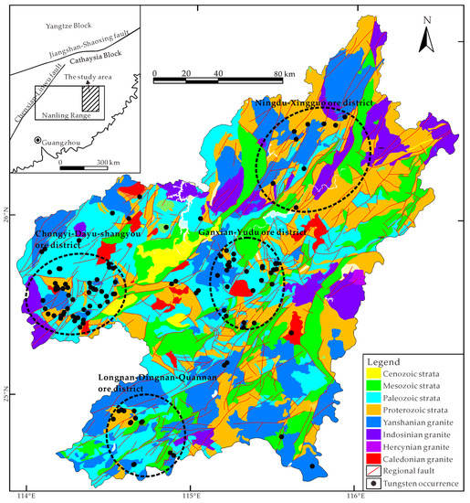
Figure 1.
Simplified geological map of southern Jiangxi Province, modified from [27,30,31].
2.2. Mineral System
In order to extract reliable targeting criteria for the subsequent prospectivity modeling, a mineral systems approach is employed to transfer understandings of tungsten mineral system into a set of mappable spatial proxies representing critical ore-forming processes related to source, transport, physical trap and chemical deposition [32,33,34,35] (Figure 2).
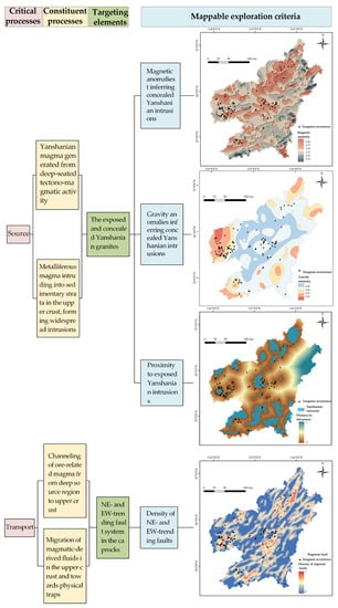
Figure 2.
Components of tungsten mineral system in the southern Jiangxi Province.
In many cases, a hydrothermal mineral system has a single source that provides not only the energy gradient, thus triggering mineralization events, but also the necessary components required for ore formation (e.g., metal, fluids and ligands) [34]. In the study area, the Yanshanian granitic intrusions are believed to play a role that provides ore-related fluids and metals, based on the understandings of previous studies. The chronological studies indicate that the formation of tungsten orebodies in the study area is temporally identical to their proximal granitic intrusions (mainly 170–150 Ma) [29,36,37]. Spatially, most of the tungsten orebodies are found at the inner and/or outer contacts of Yanshanian granitic intrusions [38,39]. Accordingly, proximity to exposed Yanshanian intrusions was employed as evidence of the source process. In addition, geophysical anomalies can provide information about buried anomalous bodies, mostly related to intrusive rocks, and therefore can be used to infer source components. Specifically, the density difference between the Yanshanian granite intrusions and their proximal Paleozoic wall rocks is approximately −100 kg/m3 [40], allowing for the detection of buried intrusions by low gravity. Intrusive rocks in this district exhibit magnetic susceptibility to a different extent [40], whereas sedimentary wall rocks have no magnetism. Thus, magnetic high is considered to be effective at tracing buried intrusions. Given that the magnetic inclination of this area is 44.6°, a reduction to the pole (RTP) transformation was applied to process the original magnetic data in order to remove the inclination effect of the Earth’s magnetic field.
Active pathways are essential for transporting ore-forming components from deep source regions to shallow trap zones [34]. As mentioned above, the Yanshanian tectono-magmatic activity is believed to be responsible for regional tungsten mineralization, while the regional fault system is believed to provide pathways for the ascent of ore-related magma. It is noteworthy that only those faults formed before or in the mineralization era can play the pathway role that promotes the mineralization process. By contrast, the faults formed after mineralization usually disconnect pre-formed ore-bearing structures and thus exert a negative impact on mineral prospecting. The previous spatial analyses indicate that the EW- and NE-trending faults, which serve as metalliferous magma-/fluid-conducting conduits, were formed or re-activated in the Yanshanian epoch [41]. The density of these faults is used to reflect transport process.
Regarding hydrothermal deposits, physical traps are favorable loci that trap ore-forming fluids. These loci are mostly related to dilatational zones induced by ore-related structural activities [42]. In the study area, EW- and NE-trending faults in the caprocks constitute transport networks for metalliferous fluids, while the intersections of these faults provide dilatational zones with high permeability that are conducive to trapping and focusing the fluids [41].
A hydrothermal deposit is the direct result of massive metal deposition. This critical process stems from the reduction in metal solubility in fluids, which is induced by a variety of sub-processes associated with changes in physical and chemical conditions [34], e.g., fluid mixing, fluid-rock reactions, and cooling of fluids. Unfortunately, it is impossible to directly trace these sub-processes from the perspective of regional-scale spatial proxies. Instead, we employ geochemical anomalies, which are footprints of ore-induced chemical sub-processes, as effective proxies of metal deposition. W, Mn and Fe are selected as targeted geochemical elements since they are components of the wolframite (Fe,Mn)WO4) that dominates the ores in the study area.
2.3. Input Dataset
An integral and reliable input dataset is an essential prerequisite for the construction of a robust machine learning-based predictive modeling. For an MPM task, the preparation of input datasets includes the data generation of evidential layers and target variables.
The evidential layers are featured predictive maps representing critical ore-forming processes. They are employed as judging conditions for the prediction of mineral potential. As mentioned above, eight evidential layers were generated on the basis of analyses of the mineral systems approach (Figure 2). The mappable intrusions, faults and geophysical anomalies were derived from the Database of Ganzhou Bureau of Geology and Mineral Resources (DGBGMR) based on field investigations since the 1980s. Geochemical anomalies of W, Mn and Fe were extracted from stream sediment data of Nanling Range, which stem from China’s National Geochemical Mapping Project with sampling density of one sample per km2 [43,44]. The eight predictor maps were generated by rasterizing mappable ore-related features. The rasterizing cell size, i.e., predictive resolution, was 450 m. This was determined based on the resolution of evidential maps and distance between any two nearest deposits [9,45,46]. A total of 195, 174 cells were generated, covering the whole study area.
The target variables of MPM include positive and negative samples used for training and testing models. A total of 118 mines, historic mines and mineralized spots representing known deposit locations were derived from DGBGMR and the online database of the China Geology Survey [31]; these were employed as positive samples. The negative samples, representing non-deposit locations, were selected based on the criteria proposed by Carranza and Zuo [47,48]. A total of 346 non-deposit locations were selected as negative samples in this study, allowing for an experiment of data imbalance.
3. Methods
3.1. Few-Shot Learning Framework
The proposed few-shot learning framework is composed of two components, including data augmentation for addressing imbalanced dataset and transfer learning for training prospectivity model by limited labeled data, as shown in Figure 3.
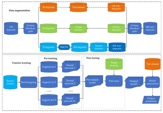
Figure 3.
Flow chart of proposed few-shot learning framework.
An imbalanced dataset consists of variable classes that are not approximately equally represented [49]. It is widely acknowledged that machine learning algorithms display poor performances in the analysis of highly imbalanced datasets [22]. However, it is a fact that non-deposit sites (negative samples) largely outnumber deposit locations (positive samples) in any case study of MPM, leading to a severe issue of imbalanced datasets. This issue can be addressed by assigning costs to training samples of different classes or by re-sampling the original dataset. The latter solution, which includes over-sampling the minority class and under-sampling the majority class, is commonly used in machine learning-based MPM. SMOTE, proven to be effective in MPM predictions [17,50], was employed in this study to over-sample minor deposits. SMOTE works by generating new synthetic samples from the existing samples of minority class based on their nearest neighbors in the feature space. As depicted in Figure 4, for a given minority-class sample Xi, k (k = 6 in this example) nearest neighboring minority-class samples are chosen. X2 is randomly selected from these four samples, and then a feature vector along the line segment between Xi and X2 is generated. A synthetic sample Xn is created by using Equation (1) [51].
where rand(0,1) denotes a random number ranging from 0 to 1.
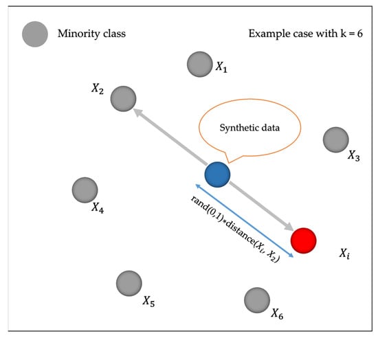
Figure 4.
Schematic description of synthetic minority over-sampling technique.
Data augmentation is task-specific and should be conducted to yield data that are well-suited to the subsequent training tasks. In this study, 20% and 15% deposit samples were randomly selected from the original dataset of positive labels. They were combined with an equal number of randomly selected non-deposits to constitute the test and target domain dataset, respectively. SOMTE was then conducted on the remaining 76 deposits and 304 non-deposits to generate a synthetically balanced dataset of the source domain (Figure 3).
Essentially, transfer learning is the reuse of a pre-trained model on a new domain. This includes two key tasks, namely, learning knowledge from a large quantity of available labeled data and transferring knowledge to a different but related problem. As mentioned above, the difficulty of finding a model of similar task transferable for training non-image-based ore-related data is the severest issue that impedes the application of transfer learning in the MPM field. In this study, the solution to this issue was to pre-train the transferable model based on the large synthetic dataset of source domain. The idea of meta-learning was introduced in the process of pre-training. Specifically, N subsets called support sets were generated by bootstrapping. Bootstrapping is a sampling procedure that randomly selects samples from the original dataset with replacement. A set of neural network models were trained by support sets, after which they were ensembled to generate a pre-trained model. The model parameters were assumed to reach a suboptimal state by multi-task pre-training in the source domain, and then a small number of samples in the target domain were used to train the model to achieve the optimal state by slightly tuning the model’s architecture [52]. Such a process is called fine-tuning. As a result of fine-tuning, the trained model displayed a satisfactory level of performance while fitting the data distribution of the target domain. The trained model was assessed with the test dataset and generated the final predictions.
3.2. Benchmark Machine Learning Algorithms
Benchmark algorithms allow for comparative study of model performance, which is strongly suggested in data-driven machine learning-based modeling [53]. Two widely applied models, namely, random forest and support vector machine, were employed as benchmark algorithms in this study.
Random forest, proposed by Breiman [54], is a classic ensemble learning algorithm that aggregates a large number of base tree models to perform repeated predictions of a specific phenomenon [1,16]. Two key random scenarios are employed to enhance the performance of model. Firstly, bootstrapping, as mentioned above, is used to create diverse subsets of original labeled data for training each base tree. Secondly, a randomly selected subset of input features is utilized to supply discriminative conditions at each node of the tree in the forest. The algorithm then searches across all the nodes to find the optimal one that maximizes the purity of the resulting trees. The purity can be measured by many indices, e.g., Gini index, Chi-square and gain ratio [16]. The final prediction is made by majority voting of all the base trees in the forest.
Support vector machine exhibits its great performance in conditional classification and operates based on theories of statistical learning and structural risk minimization [47,55,56]. The algorithm seeks to generate an optimal classifier that separates labels of different classes with the widest discriminative boundaries. This algorithm works by finding a hyperplane that has the largest margin in the feature space, i.e., the distance between the hyperplane and its closest data points of each class is at a maximum, which allows for the generation of a classier with the lowest errors [57,58].
Since benchmark algorithms are not the main theme of this study, only a brief introduction is presented above. Detailed descriptions of the algorithms can be referred to [47,54,55,56,57,58].
3.3. Performance Metric
The model performance can be evaluated by a set of quantitative measurements. The indices employed in this study demonstrate their capability to assess the robustness and predictive efficiency of the models.
Classification accuracy is used to rapidly appraise the effect of parameter optimization. It can be calculated by determining the ratio of the number of correctly classified samples to the total number of the samples; however, this index fails to evaluate the predictive performance of the model. The receiver operating characteristic (ROC) curve and success rate curve are used to measure the overall predictive performance of the model. These curves are drawn based on the varying discriminative thresholds that define the predictive results of a binary classification system [59,60]. A cell with a probability value greater or lower than the discriminative threshold is predicted to be a deposit or non-deposit. The sensitivity and specificity are computed by Equations (2) and (3) [61].
where TP represents a result whereby a deposit is correctly predicted as a deposit; FN means that a deposit is incorrectly predicted as a non-deposit; TN depicts a result whereby a non-deposit is correctly predicted as a non-deposit; and FP represents a result whereby a non-deposit is incorrectly predicted as a deposit. The ROC curve is generated by plotting sensitivity on the y axis against (1-specificity) on the x axis at gradually decreasing discriminative thresholds. The closer the ROC curve inflects towards the upper left corner, the better the model performs [62]. Such criteria can be quantified by the area under the curve (AUC), which ranges from 0 (the poorest performance) to 1 (perfect prediction). The success rate is the ratio of the number of deposits contained in the targeting regions to the total number of deposits. The success rate curve is generated by plotting the success rate on the y axis against the area percentage of targeting regions on the x axis at gradually decreasing discriminative thresholds.
In this study, the over-fitting of a predictive model is quantified by two indices, i.e., bias and variance. Bias is linked to the ability of a model to fit the labeled data of training dataset, while variance is related to the ability of a model to correlate with those labeled samples excluded from a training dataset [4,63,64]. Given that the AUC is used to assess overall predictive performance, the values of (1-AUC), calculated on the training and test dataset, are used to estimate bias and variance, respectively. The difference between bias and variance can be regarded as a quantitative measurement of over-fitting [65]. In order to measure the uncertainty of predictive results, 10-time randomly splitting of the original data was implemented together with bootstrapping, resulting in 10 predictive models. The mean and standard deviation of predictive values in each cell were considered as modulated predictive values and quantitative uncertainty.
Information gain (IG) was used to quantify the contribution of each featured layer to the trained model, which can be calculated by the following formula [66].
where Y is output class (deposit or non-deposit); Fi represents a specific featured layer; H(Y) is the entropy value of Y; and H(Y|Fi) is the entropy value Y after associating the feature values of Fi (see [66] for details).
4. Results
4.1. Data Imbalancing Analysis of SMOTE Augmentation
SMOTE was used in this study to augment minor positive samples to balance the training dataset. In order to reveal the effectiveness of data augmentation and determine the optimum composition of training dataset, a grid search procedure was implemented on 182 SMOTE-ed training datasets involving variable over-sampling and under-sampling rates. The accuracies of the trained models were calculated to measure their performances, as shown in Figure 5a.
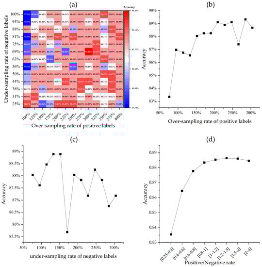
Figure 5.
Results of data imbalance analyses: (a) classification accuracies of model trained by various combinations of over-sampling and under-sampling rate; (b) accuracy curve regarding varying over-sampling rate; (c) accuracy curve regarding varying under-sampling rate; (d) accuracy curve regarding positive/negative rate.
The models with the lowest accuracies were those trained by datasets with low positive over-sampling rates and high negative under-sampling rates, mostly occupying the upper left corner of the graph. In contrast, the models with the highest accuracies generally had high positive over-sampling rates, occurring in the right half of the graph. The impact of individual sampling rate on model performance was further delineated by the statistical results of the accuracies of models that took a specific positive over-sampling rate or negative under-sampling rate (Figure 5b,c). The results indicate that the accuracies generally increased as the positive over-sampling rate increased, whereas the models’ performance became more unfavorable with the increasing negative under-sampling rate. More specifically, the rates of positive samples to negative samples were grouped into eight intervals to test the reasonable positive/negative ratio employed in the training dataset. The result indicates that the accuracies consistently increased as the positive/negative rate increased at the interval between 0.25 and 1, after which the models’ accuracies achieved a stably high level (Figure 5d). The above results suggest that models trained by datasets with high positive to negative ratios, i.e., greater than 1, tended to be more accurate and stable. In light of the criteria inferred from previous data-balancing studies [17], it seems that 1:1 balanced positive and negative samples generalize better model performance. Therefore, a dataset including 228 positive samples and 209 negative samples, which yielded the best model accuracy of 94.44% in this study (Figure 5a), was employed to train the FSL models.
4.2. Assessment of Model Precision and Generalization
A random data split procedure was used 10 times to create 10 different sub-datasets, allowing us to measure the overall performance and stochastic uncertainty of few-shot learning models in a robust way. RF and SVM models, which served as benchmark models in this study, were also generated from 10 random selected training datasets. For each algorithm, the resulting probability and uncertainty values of the 10 trained models were normalized to a [0–1] range (Figure 6, Figure 7, Figure 8, Figure 9 and Figure 10), allowing for a comparative analysis.
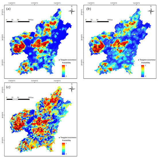
Figure 6.
Predictive maps showing average probability yielded by: (a) few-shot learning models; (b) random forest models; (c) support vector machine models.
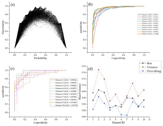
Figure 7.
Model performance of few-shot learning models: (a) scatter plot showing probability versus their quantified uncertainty; (b) ROC curves for training datasets; (c) ROC curves for test datasets; (d) measurement of over-fitting on different datasets.
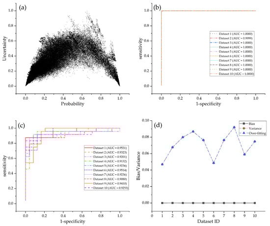
Figure 8.
Model performance of random forest models: (a) scatter plot showing probability versus their quantified uncertainty; (b) ROC curves for training datasets; (c) ROC curves for test datasets; (d) measurement of over-fitting on different datasets.
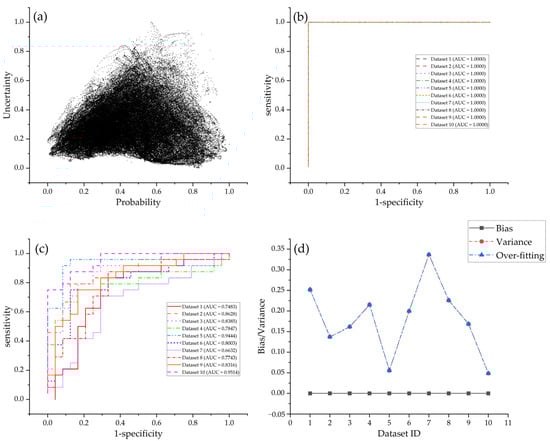
Figure 9.
Model performance of support vector machine models: (a) scatter plot showing probability versus their quantified uncertainty; (b) ROC curves for training datasets; (c) ROC curves for test datasets; (d) measurement of over-fitting on different datasets.
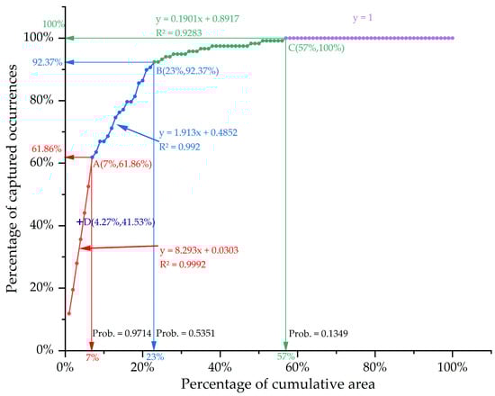
Figure 10.
Success rate curve of few-shot learning predictive model (Probability is abbreviated as Prob.).
FSL and RF models output arch-shaped point patterns in graphs of uncertainty versus probability (Figure 7a and Figure 8a). This pattern shows that the cells with low uncertainty either have a high mineralization probability or are close to zones of a low prospectivity, whereas those cells with moderate probability have high uncertainty. The points derived from SVM models are irregular. The cells with low uncertainty have probability values that vary from 0 to 1, with no clustering trends towards the lowest- or the highest-probability zones (Figure 9a). For a mineral explorers, the arch-shaped point pattern is more favorable for prospectivity mapping as their attention is more focused on high-probability cells, which are first-order targets of future exploration, as well as on low-probability cells that should be excluded from target selection. Conversely, these focused cells with low uncertainty are deemed robust and low-risk targets.
The ROC curves for the three machine learning algorithms show marked differences (Figure 7, Figure 8 and Figure 9). Two patterns of ROC curves are identified when the models are verified by training datasets, i.e., a perfect predictive curve with an AUC equal to 1 (for RF and SVM models, shown in Figure 8b and Figure 9b) and a step-shaped curve with an AUC varying from 0.9 to 1 (for FSL models, shown in Figure 7b). In contrast, all the three algorithms yield step-shaped curves when trained by test datasets. These patterns clearly show that RF and SVM models fall into the trap of over-fitting, which exhibits a perfect predictive performance on training datasets but fails to completely generalize using test datasets. Although the ROC curves of FSL models on both training and test datasets show step-shaped patterns, these models also suffer from over-fitting given that the AUCs of training datasets are greater than those of test datasets (Figure 7b,c). The over-fitting is quantified by bias and variance, as depicted in Figure 7d, Figure 8d and Figure 9d and Table 1. RF models have the lowest average variance, implying the superior performance of RF models on test datasets (average AUC = 0.9292); they are followed by FSL models, which also achieve high AUCs on test datasets (average AUC = 0.9172). FSL models have the lowest measured value of over-fitting (0.0313), which is far lower than that of RF (0.0708) and SVM models (0.1801).

Table 1.
Comparison of model generalization.
4.3. Targets of Predictive Modeling
Aiming to generate a robust prospectivity map with lowest uncertainty, the FSL models are chosen as the final predictive models. However, it is still a challenging task to extract the optimal exploration targets from resulting FSL models. Reliance on excessively extensive prospective zones would greatly increase exploration costs, whereas the use of too limited targeting zones would reduce the success rate of prospecting. Therefore, predictive efficiency, considering both success rate and delineated area, is essential for the targeting task. A success rate curve is employed here to measure the predictive efficiency of the proposed models, as shown in Figure 10. Four segments of success rate curves are clearly identified with fitting coefficients greater than 0.92. Given that the slope of the fitting curve indicates the ratio of successfully predicted deposits versus the delimited area, it can be employed as an effective means of quantifying the predictive efficiency. The first segment of success rate curve represents the predictive efficiency of those cells with top probabilities, thus reflecting the most important aspect of a model’s predictive efficiency. The slope of the first segment of success rate curve is 8.293, with high coefficient of determination of 0.9992. The end point of the first segment or the intersection point of the first and the second segments (Point A in Figure 10) corresponds to 7% of the cumulative area on the x axis and 61.86% of included deposits on the y axis, indicating that 61.86% of known mineral deposits are captured within 7% of the study area. This result is superior to the best predictive efficiency of 6.7797 yielded from previous MPM modeling in this region [9]. The slopes of the second and the third segments of the success rate curve dramatically decrease to 1.913 and 0.1901, respectively, depicting rapid decline in predictive efficiency with decreasing probability.
Different slopes of success rate curves suggest different predictive efficiencies. Thus, the intersections of different segments of success rate curves (i.e., Points A, B and C in Figure 10) imply possible threshold values for the classification of different prospectivity levels. In this regard, four levels of mineral prospectivity, namely, high potential, moderate potential, low potential, and barren zones, are identified from Figure 10, based on which a prospectivity map is generated (Figure 11). Uncertainty is employed to further estimate the reliability of predictive results, reducing exploration risk. However, there is no common criteria for selecting threshold value for masking high uncertain cells [4]. In this study, four levels of uncertainty, namely, very high, high, medium and low, are determined based on the threshold values of three quartiles of uncertainty values. Considering both predictive efficiency and exploration risk, the final targets for future exploration fall on the cells with high potential and low uncertainty, as shown with the brownfield zone in Figure 12. This zone represents updated targets from the high-potential regions, which can be projected to Point D in Figure 10, located above the first segment. The final low-risk exploration targets only cover 4.27% of the area but capture 41.53% of known tungsten deposits (Figure 11), achieving the best predictive efficiency of 9.7155.
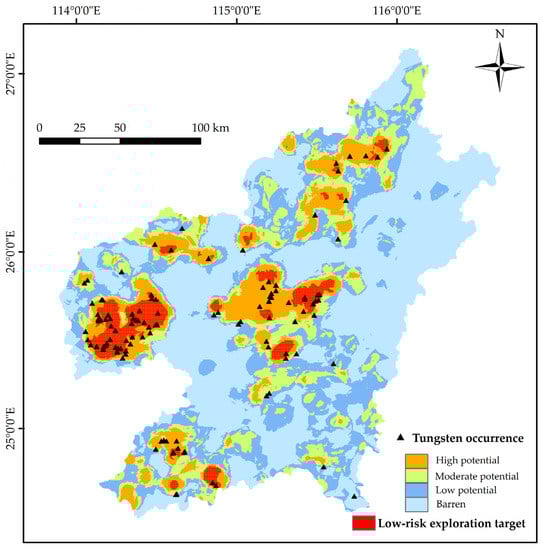
Figure 11.
Prospectivity map showing different potential areas and low-risk exploration targets.
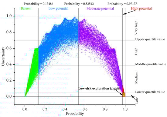
Figure 12.
Zoning of scatter plot based on threshold values of both probability and uncertainty.
5. Discussion
The objective of using MPM in this study was to generate a robust predictive model with low uncertainty, thus reducing the future exploration risk to the maximum extent. To achieve this goal, three aspects of scenarios were implemented.
Geologically, the mineral systems approach was employed to translate our understanding of the tungsten mineral system into mappable exploration criteria, resulting in 8 evidential maps that represent the source, transport, physical trap and chemical deposition processes critical to ore formation. The feature weights of evidential layers, measured by information gain, imply that most selected evidence makes major or significant contributions to the final predictions (Figure 13). As a direct indication of targeted mineralization, W anomalies impose the greatest influence on the predictive results. Proximity to Yanshanian intrusions and density of fault intersections, corresponding to spatial proxies of ore-forming parent magmatic rocks and regional structural that have been rightly recognized as ore-controlling factors, exert important influence on the predictions. It is interesting to observe that Mn anomalies make equal contributions to prediction as above-mentioned well-recognized elements, which is consistent with our previous study [9], implying that Mn derived from host rocks may exert a significant control on wolframite precipitation. Magnetic anomalies, fault density and Fe anomalies make secondary contributions to predictions. It is worth noting that gravity anomalies are interpreted as contributing little to predictive results, implying their failure in spatially representing buried intrusions. This raises a limitation problem of this study based on 2D maps, namely, the lack of evidential layers that can effectively portray ore-related processes at depth. Three-dimensional inversions of geophysical anomalies derived from high-resolution gravity, magnetic and resistivity data are excellent solutions to this problem. They are efficient at tracing intrusive rocks, fault network and ore-controlling/-bearing structures at depth [65,67]. Unfortunately, such data are costly and generally available at deposit-scale; thus, they cannot be utilized in a regional-scale MPM at present. Integrating such evidence into future work would improve the effectiveness of predictor maps and boost the performance of predictive models.
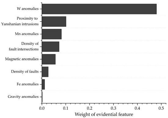
Figure 13.
Feature weights obtained by information gain.
Algorithmically, an FSL framework jointly employing data augmentation and transferring was proposed as this method appears to be effective at controlling over-fitting regarding model assessment (Figure 7 and Table 1). On the one hand, 10-time random data splitting was implemented, and bootstrapping was carried out based on the augmented data derived from a robust SMOTE algorithm. This multi-round random scenario not only provided a means of quantifying uncertainty and reducing fluctuation of predictive results but also greatly increased the diversity of input datasets and pre-trained models. Thus, we prevented the models from excessively over-fitting. On the other hand, the augmented synthetic data created a data-rich source domain. Meanwhile, they were intrinsically correlated with the labeled data in the target domain, which benefited the transfer of the knowledge obtained from source domain to the target domain, thereby enhancing the generalization capability of these models. In this regard, the FSL model cam be considered as the optimal one that can be well generalized for further exploration targeting.
Practically, this study employed performance metrics, linking predictive results to realistic mineral exploration activity. The confusion matrix-based indices are usually employed to assess the accuracy of binary classification. However, in this study, they were only used to rapidly measure the effect of parameter optimization but were not taken into account for performance evaluation. The reason for this was that the confusion matrix of binary classification takes 0.5 as a common threshold. The cell greater or lower than 0.5 is labeled as positive or negative. In the MPM field, the inclusion of such a criterion leads to excessively extensive “favorable regions” (often beyond 30% of the study area), which conflicts with one of the basic principles of mineral exploration, namely, narrowing down the area of exploration targets. Instead, performance metrics based on varying discriminative thresholds, i.e., ROC curve and success rate curve, were employed in this study, and attention were especially focused on the high-probability and low-uncertainty zones. The final targets, capturing 49 out of 118 known deposits within only 4.27% of the total area, allowed for an efficient and realistic exploration plan for future tungsten prospecting in this area.
6. Conclusions
A prospectivity map, generated from a robust modeling process, is crucial for efficient exploration targeting. In this study, we proposed an FSL framework, combining the mineral systems approach, SMOTE augmentation algorithm, transfer learning and performance metrics linked to realistic mineral exploration, and applied it in tungsten prospectivity mapping of southern Jiangxi Province. The resulting predictive model generated an arch-shaped point distribution pattern in the scatter plot of probability and uncertainty, which was favorable for selecting potential targets with high probability and low uncertainty; achieved a high AUC value of 0.9172 on the test dataset; and yielded the lowest quantitative over-fitting value compared to benchmark machine learning algorithms. The predictive results demonstrate the excellent performance of the proposed framework in controlling over-fitting and generating high-potential, low-risk exploration targets. The final exploration targets only covered 4.27% of the area, but captured 41.53% of known tungsten deposits, providing a significant reference for further tungsten prospecting in the study area.
Author Contributions
Conceptualization, T.S.; methodology, K.Z., T.S. and Y.L.; validation, K.Z. and M.F.; formal analysis, W.P. and J.T.; investigation, Y.L. and K.Z.; resources, J.H. and L.M.; writing—original draft preparation, K.Z. and T.S.; visualization, K.Z.; project administration, T.S.; funding acquisition, T.S. All authors have read and agreed to the published version of the manuscript.
Funding
This research was funded by National Natural Science Foundation of China (Grant Nos. 42062021 and 41963005); Natural Science Foundation of Jiangxi Province for Distinguished Young Scholars (Grant No. 20224ACB218003); China Postdoctoral Science Foundation (Grant No. 2019M662267); Natural Science Foundation of Jiangxi Province (Grant No. 20202BAB203016); Program of Qingjiang Excellent Young Talents, Jiangxi University of Science and Technology (Grant No. JXUSTQJBJ2020001); and Science and Technology Program of Ganzhou City (Grant No. 202101095156).
Data Availability Statement
The data presented in this study are not publicly available due to privacy.
Acknowledgments
We are grateful to two anonymous reviewers for their constructive comments that significantly improved the manuscript. We thank RapidMiner Team for their technical support via RapidMiner Studio.
Conflicts of Interest
The authors declare no conflict of interest.
References
- Carranza, E.J.M.; Laborte, A.G. Data-driven predictive mapping of gold prospectivity, Baguio district, Philippines: Application of Random Forests algorithm. Ore Geol. Rev. 2015, 71, 777–787. [Google Scholar] [CrossRef]
- Daviran, M.; Maghsoudi, A.; Ghezelbash, R.; Pradhan, B. A new strategy for spatial predictive mapping of mineral prospectivity: Automated hyperparameter tuning of random forest approach. Comput. Geosci. 2021, 148, 104688. [Google Scholar] [CrossRef]
- Zuo, R.G. Geodata Science-Based Mineral Prospectivity Mapping: A Review. Nat. Resour. Res. 2020, 29, 3415–3424. [Google Scholar] [CrossRef]
- Parsa, M.; Lentz, D.R.; Walker, J.A. Predictive Modeling of Prospectivity for VHMS Mineral Deposits, Northeastern Bathurst Mining Camp, NB, Canada, Using an Ensemble Regularization Technique. Nat. Resour. Res. 2022, 32, 19–36. [Google Scholar] [CrossRef]
- Hu, X.; Li, X.; Yuan, F.; Ord, A.; Jowitt, S.M.; Li, Y.; Dai, W.; Zhou, T. Numerical Modeling of Ore-forming Processes within the Chating Cu-Au Porphyry-type Deposit, China: Implications for the Longevity of Hydrothermal Systems and Potential Uses in Mineral Exploration. Ore Geol. Rev. 2020, 116, 103230. [Google Scholar] [CrossRef]
- Hu, X.; Chen, Y.; Liu, G.; Yang, H.; Luo, J.; Ren, K.; Yang, Y. Numerical modeling of formation of the Maoping Pb-Zn deposit within the Sichuan-Yunnan-Guizhou Metallogenic Province, southwestern China: Implications for the spatial distribution of concealed Pb mineralization and its controlling factors. Ore Geol. Rev. 2022, 140, 104573. [Google Scholar] [CrossRef]
- Qin, Y.; Liu, L. Quantitative 3D Association of Geological Factors and Geophysical Fields with Mineralization and Its Significance for Ore Prediction: An Example from Anqing Orefield, China. Minerals 2018, 8, 300. [Google Scholar] [CrossRef]
- Hu, X.; Liu, G.; Chen, Y.; Luo, J.; Yang, H.; Yang, Y.; Ren, K.; Li, Y.; Gao, L. Combination model-based numerical simulation of the mineralizing processes within iron oxide-apatite systems. Ore Geol. Rev. 2023, 156, 105394. [Google Scholar] [CrossRef]
- Sun, T.; Li, H.; Wu, K.; Chen, F.; Zhu, Z.; Hu, Z. Data-Driven Predictive Modelling of Mineral Prospectivity Using Machine Learning and Deep Learning Methods: A Case Study from Southern Jiangxi Province, China. Minerals 2020, 10, 102. [Google Scholar] [CrossRef]
- Zuo, R.G.; Wang, Z.Y. Effects of Random Negative Training Samples on Mineral Prospectivity Mapping. Nat. Resour. Res. 2020, 29, 3443–3455. [Google Scholar] [CrossRef]
- Meng, F.; Li, X.; Chen, Y.; Ye, R.; Yuan, F. Three-Dimensional Mineral Prospectivity Modeling for Delineation of Deep-Seated Skarn-Type Mineralization in Xuancheng–Magushan Area, China. Minerals 2022, 12, 1174. [Google Scholar] [CrossRef]
- Zhang, S.; Carranza, E.J.M.; Wei, H.; Xiao, K.; Yang, F.; Xiang, J.; Zhang, S.H.; Xu, Y. Data-driven Mineral Prospectivity Mapping by Joint Application of Unsupervised Convolutional Auto-encoder Network and Supervised Convolutional Neural Network. Nat. Resour. Res. 2021, 30, 1011–1031. [Google Scholar] [CrossRef]
- Silva dos Santos, V.; Gloaguen, E.; Hector Abud Louro, V.; Blouin, M. Machine Learning Methods for Quantifying Uncertainty in Prospectivity Mapping of Magmatic-Hydrothermal Gold Deposits: A Case Study from Juruena Mineral Province, Northern Mato Grosso, Brazil. Minerals 2022, 12, 941. [Google Scholar] [CrossRef]
- Qin, Y.Z.; Liu, L.M.; Wu, W.C. Machine Learning-Based 3D Modeling of Mineral Prospectivity Mapping in the Anqing Orefield, Eastern China. Nat. Resour. Res. 2020, 29, 3099–3120. [Google Scholar] [CrossRef]
- Porwal, A.; Carranza, E.J.M. Introduction to the special issue: GIS-based mineral potential modelling and geological data analyses for mineral exploration. Ore Geol. Rev. 2015, 71, 477–483. [Google Scholar] [CrossRef]
- Rodriguez-Galiano, V.; Sanchez-Castillo, M.; Chica-Olmo, M.; Chica-Rivas, M. Machine learning predictive models for mineral prospectivity: An evaluation of neural networks, random forest, regression trees and support vector machines. Ore Geol. Rev. 2015, 71, 804–818. [Google Scholar] [CrossRef]
- Prado, E.M.G.; Filho, C.R.S.; Carranza, E.J.M.; Motta, J.G.M. Modeling of Cu-Au prospectivity in the Carajás mineral province (Brazil) through machine learning: Dealing with imbalanced training data. Ore Geol. Rev. 2020, 184, 103611. [Google Scholar] [CrossRef]
- Sun, T.; Chen, F.; Zhong, L.; Liu, W.; Wang, Y. GIS-based mineral prospectivity mapping using machine learning methods: A case study from Tongling ore district, eastern China. Ore Geol. Rev. 2019, 109, 26–49. [Google Scholar] [CrossRef]
- Zuo, R.G.; Kreuzer, O.P.; Wang, J.; Xiong, Y.H.; Zhang, Z.J.; Wang, Z.Y. Uncertainties in GIS-Based Mineral Prospectivity Mapping: Key Types, Potential Impacts and Possible Solutions. Nat. Resour. Res. 2021, 30, 3059–3079. [Google Scholar] [CrossRef]
- Wu, J.Y.; Zhao, Z.B.; Sun, C.; Yan, R.Q.; Chen, X.F. Few-shot transfer learning for intelligent fault diagnosis of machin. Measurement 2020, 166, 108202. [Google Scholar] [CrossRef]
- Sun, X.; Wang, B.; Wang, Z.R.; Li, H.; Li, H.C.; Fu, K. Research Progress on Few-Shot Learning for Remote Sensing Image Interpretation. IEEE J. Sel. Top. Appl. Earth Obs. Remote Sens. 2021, 14, 2387–2402. [Google Scholar] [CrossRef]
- Hariharan, S.; Tirodkar, S.; Porwal, A.; Bhattacharya, A.; Joly, A. Random Forest-Based Prospectivity Modelling of Greenfield Terrains Using Sparse Deposit Data: An Example from the Tanami Region, Western Australia. Nat. Resour. Res. 2017, 26, 489–507. [Google Scholar] [CrossRef]
- Li, T.; Xia, Q.; Zhao, M.; Gui, Z.; Leng, S. Prospectivity Mapping for Tungsten Polymetallic Mineral Resources, Nanling Metallogenic Belt, South China: Use of Random Forest Algorithm from a Perspective of Data Imbalance. Nat. Resour. Res. 2019, 29, 203–227. [Google Scholar] [CrossRef]
- Li, H.; Li, X.H.; Yuan, F.; Jowitt, S.M.; Zhang, M.M.; Zhou, J.; Zhou, T.F.; Li, X.L.; Ge, C.; Wu, B.C. Convolutional neural network and transfer learning based mineral prospectivity modeling for geochemical exploration of Au mineralization within the Guandian–Zhangbaling area, Anhui Province, China. Appl. Geochem. 2020, 122, 104747. [Google Scholar] [CrossRef]
- Wu, B.C.; Li, X.H.; Yuan, F.; Li, H.; Zhang, M.M. Transfer learning and siamese neural network based identification of geochemical anomalies for mineral exploration: A case study from the Cu–Au deposit in the NW Junggar area of northern Xinjiang Province, China. J. Geochem. Explor. 2022, 232, 106904. [Google Scholar] [CrossRef]
- Ding, K.; Xue, L.F.; Ran, X.J.; Wang, J.B.; Yan, Q. Siamese network based prospecting prediction method: A case study from the Au deposit in the Chongli mineral concentrate area in Zhangjiakou, Hebei Province, China. Ore Geol. Rev. 2022, 148, 105024. [Google Scholar] [CrossRef]
- Feng, C.Y.; Zeng, Z.L.; Zhang, W.J.; Qu, W.J.; Du, A.D.; Li, D.X.; She, H.Q. SHRIMP zircon U–Pb and molybdenite Re–Os isotopic dating of the tungsten deposits in the Tianmenshan–Hongtaoling W–Sn orefield, southern Jiangxi Province, China, and geological implications. Ore Geol. Rev. 2011, 43, 8–25. [Google Scholar] [CrossRef]
- Mao, J.; Cheng, Y.; Chen, M.; Pirajno, F. Major types and time–space distribution of Mesozoic ore deposits in south China and their geodynamic settings. Miner. Depos. 2013, 48, 267–294. [Google Scholar]
- Feng, C.; Zhang, D.; Zeng, Z.; Wang, S. Chronology of the tungsten deposits in southern Jiangxi Province, and episodes and zonation of the regional W-Sn mineralization-evidence from high-precision zircon U-Pb, molybdenite Re-Os and muscovite Ar-Ar ages. Acta Geol. Sin.-Engl. Ed. 2012, 86, 555–567. [Google Scholar]
- Fang, G.; Chen, Z.; Chen, Y.; Li, J.; Zhao, B.; Zhou, X.; Zeng, Z.; Zhang, Y. Geophysical investigations of the geology and structure of the Pangushan-Tieshanlong tungsten ore field, South Jiangxi, China—Evidence for site-selection of the 2000-m Nanling scientific drilling project (SP-NLSD-2). J. Asian Earth Sci. 2015, 110, 10–18. [Google Scholar] [CrossRef]
- GeoCloud Database of China Geological Survey. Available online: http://geocloud.cgs.gov.cn (accessed on 25 April 2023).
- Wyborn, L.A.I.; Heinrich, C.A.; Jaques, A.L. Australian Proterozoic mineral systems: Essential ingredients and mappable criteria. Australas. Inst. Min. Metall. Publ. Ser. 1994, 5, 109–115. [Google Scholar]
- Kreuzer, O.P.; Miller, A.V.M.; Peters, K.J.; Payne, C.; Wildman, C.; Partington, G.A.; Puccioni, E.; McMahon, M.E.; Etheridge, M.A. Comparing prospectivity modelling results and past exploration data: A case study of porphyry Cu–Au mineral systems in the Macquarie Arc, Lachlan Fold Belt, New South Wales. Ore Geol. Rev. 2015, 71, 516–544. [Google Scholar] [CrossRef]
- Hagemann, S.G.; Lisitsin, V.A.; Huston, D.L. Mineral system analysis: Quo vadis. Ore Geol. Rev. 2016, 76, 504–522. [Google Scholar] [CrossRef]
- McCuaig, T.C.; Beresford, S.; Hronsky, J. Translating the mineral systems approach into an effective exploration targeting system. Ore Geol. Rev. 2010, 38, 128–138. [Google Scholar] [CrossRef]
- Yang, J.H.; Kang, L.F.; Peng, J.T.; Zhong, H.; Gao, J.F.; Liu, L. In-situ elemental and isotopic compositions of apatite and zircon from the Shuikoushan and Xihuashan granitic plutons: Implication for Jurassic granitoid-related Cu-Pb-Zn and W mineralization in the Nanling Range, south China. Ore Geol. Rev. 2018, 93, 382–403. [Google Scholar] [CrossRef]
- Yang, J.H.; Kang, L.F.; Liu, L.; Peng, J.T.; Qi, Y.Q. Tracing the origin of ore-forming fluids in the Piaotang tungsten deposit, south China: Constraints from in-situ analyses of wolframite and individual fluid inclusion. Ore Geol. Rev. 2019, 111, 102939. [Google Scholar] [CrossRef]
- Zhao, W.W.; Zhou, M.F.; Li, Y.H.M.; Zhao, Z.; Gao, J.F. Genetic types, mineralization styles, and geodynamic settings of Mesozoic tungsten deposits in south China. J. Asian Earth Sci. 2017, 137, 109–140. [Google Scholar] [CrossRef]
- Liang, X.; Dong, C.; Jiang, Y.; Wu, S.; Zhou, Y.; Zhu, H.; Fu, J.; Wang, C.; Shan, Y. Zircon U–Pb, molybdenite Re–Os and muscovite Ar–Ar isotopic dating of the XitianW–Sn polymetallic deposit, eastern Hunan Province, south China and its geological significance. Ore Geol. Rev. 2016, 78, 85–100. [Google Scholar] [CrossRef]
- Editorial Committee of China Mineral Geological Record. The Mineral Geological Records of China: Volume of Jiangxi Province; Geology Publishing House: Beijing, China, 2015; pp. 967–976. (In Chinese) [Google Scholar]
- Nanling Range Group of Ministry of Geology and Mineral Resources. Study on Regional Tectonic Characteristics and Ore-Forming Structures in the Nanling Range; Geology Publishing House: Beijing, China, 1988; pp. 102–134. (In Chinese) [Google Scholar]
- Joly, A.; Porwal, A.; McCuaig, T.C. Exploration targeting for orogenic gold deposits in the Granites-Tanami Orogen: Mineral system analysis, targeting model and prospectivity analysis. Ore Geol. Rev. 2012, 48, 349–383. [Google Scholar] [CrossRef]
- Chen, X.; Fu, J. Geochemical Maps of Nanling Range; China University of Geoscience Press: Wuhan, China, 2012; pp. 50–109. (In Chinese) [Google Scholar]
- Xie, X.J.; Mu, X.Z.; Ren, T.X. Geochemical mapping in China. J. Geochem. Explor. 1997, 60, 99–113. [Google Scholar]
- Carranza, E.J.M. Objective selection of suitable unit cell size in data-driven modeling of mineral prospectivity. Comput. Geosci. 2009, 35, 2032–2046. [Google Scholar] [CrossRef]
- Hengl, T. Finding the right pixel size. Comput. Geosci. 2006, 32, 1283–1298. [Google Scholar] [CrossRef]
- Zuo, R.; Carranza, E.J.M. Support vector machine: A tool for mapping mineral prospectivity. Comput. Geosci. 2011, 37, 1967–1975. [Google Scholar] [CrossRef]
- Carranza, E.J.M.; Hale, M.; Faassen, C. Selection of coherent deposit-type locations and their application in data-driven mineral prospectivity mapping. Ore Geol. Rev. 2008, 33, 536–558. [Google Scholar] [CrossRef]
- Chawla, N.V.; Bowyer, K.W.; Hall, L.O.; Kegelmeyer, W.P. SMOTE: Synthetic Minority Over-sampling Technique. J. Artif. Intell. Res. 2002, 16, 321–357. [Google Scholar] [CrossRef]
- Shahinfar, S.; Al-Mamun, H.A.; Park, B.; Kim, S.; Gondro, C. Prediction of marbling score and carcass traits in Korean Hanwoo beef cattle using machine learning methods and synthetic minority oversampling technique. Meat Sci. 2020, 161, 107997. [Google Scholar] [CrossRef] [PubMed]
- Sohrawordi, M.; Hossain, M.A. Prediction of lysine formylation sites using support vector machine based on the sample selection from majority classes and synthetic minority over-sampling techniques. Biochimie 2022, 192, 125–135. [Google Scholar] [CrossRef]
- Jia, S.; Jiang, S.G.; Lin, Z.J.; Meng, X.; Yu, S.Q. A survey: Deep learning for hyperspectral image classification with few labeled samples. Neurocomputing 2021, 448, 179–204. [Google Scholar] [CrossRef]
- Carranza, E.J.M.; van Ruitenbeek, F.J.A.; Hecker, C.; van der Meijde, M.; van der Meer, F.D. Knowledge-guided data-driven evidential belief modeling of mineral prospectivity in Cabo de Gata, SE Spain. Int. J. Appl. Earth Obs. Geoinf. 2008, 10, 374–387. [Google Scholar] [CrossRef]
- Breiman, L. Random forests. Mach. Learn. 2001, 45, 5–32. [Google Scholar] [CrossRef]
- Vapnik, V. The Nature of Statistical Learning Theory; Springer: Berlin/Heidelberg, Germany, 2000; pp. 302–314. [Google Scholar]
- Shabankareh, M.; Hezarkhani, A. Application of support vector machines for copper potential mapping in Kerman region, Iran. J. Afr. Earth Sci. 2017, 128, 116–126. [Google Scholar] [CrossRef]
- Mahvash Mohammadi, N.; Hezarkhani, A. Application of support vector machine for the separation of mineralised zones in the Takht-e-Gonbad porphyry deposit, SE Iran. J. Afr. Earth Sci. 2018, 143, 301–308. [Google Scholar] [CrossRef]
- Asadi, H.H.; Hale, M. A predictive GIS model for mapping potential gold and base metal mineralization in Takab area, Iran. Comput. Geosci. 2001, 27, 901–912. [Google Scholar] [CrossRef]
- Nykänen, V.; Lahti, I.; Niiranen, T.; Korhonen, K. Receiver operating characteristics (ROC) as validation tool for prospectivity models—A magmatic Ni–Cu case study from the Central Lapland Greenstone Belt, Northern Finland. Ore Geol. Rev. 2015, 71, 853–860. [Google Scholar] [CrossRef]
- Nykänen, V.; Niiranen, T.; Molnár, F.; Lahti, I.; Korhonen, K.; Cook, N.; Skyttä, P. Optimizing a knowledge-driven prospectivity model for gold deposits within Peräpohja Belt, Northern Finland. Nat. Resour. Res. 2017, 26, 571–584. [Google Scholar] [CrossRef]
- Liu, C.; Berry, P.M.; Dawson, T.P.; Pearson, R.G. Selecting thresholds of occurrence in the prediction of species distributions. Ecography 2005, 28, 385–393. [Google Scholar] [CrossRef]
- Truong, X.; Mitamura, M.; Kono, Y.; Raghavan, V.; Yonezawa, G.; Truong, X.; Do, T.; Tien Bui, D.; Lee, S. Enhancing prediction performance of landslide susceptibility model using hybrid machine learning approach of bagging ensemble and logistic model tree. Appl. Sci. 2018, 8, 1046. [Google Scholar] [CrossRef]
- Parsa, M.; Carranza, E.J.M.; Ahmadi, B. Deep GMDH Neural Networks for Predictive Mapping of Mineral Prospectivity in Terrains Hosting Few but Large Mineral Deposits. Nat. Resour. Res. 2021, 31, 37–50. [Google Scholar] [CrossRef]
- Kuhn, M.; Johnson, K. Applied Predictive Modeling; Springer: Berlin/Heidelberg, Germany, 2013; pp. 13–26. [Google Scholar]
- Yan, J.Y.; Lü, Q.T.; Chen, M.C.; Deng, Z.; Qi, G.; Zhang, K.; Liu, Z.D.; Wang, J.; Liu, Y. Identification and extraction of geological structure information based on multi-scale edge detection of gravity and magnetic fields: An example of the Tongling ore concentration area. Chin. J. Geophys. 2015, 58, 4450–4464, (In Chinese with English abstract). [Google Scholar]
- Tien Bui, D.; Ho, T.C.; Pradhan, B.; Pham, B.T.; Nhu, V.H.; Revhaug, I. GIS-based modelling of rainfall-induced landslides using data mining-based functional trees classifier with AdaBoost, Bagging, and MultiBoost ensemble frameworks. Environ. Earth Sci. 2016, 75, 1101. [Google Scholar] [CrossRef]
- Li, X.; Yuan, F.; Zhang, M.; Jia, C.; Jowitt, S.M.; Ord, A.; Zheng, T.; Hu, X.; Li, Y. Three-dimensional mineral prospectivity modelling for targeting of concealed mineralization within the Zhonggu iron orefield, Ningwu Basin, China. Ore Geol. Rev. 2015, 71, 633–654. [Google Scholar] [CrossRef]


Disclaimer/Publisher’s Note: The statements, opinions and data contained in all publications are solely those of the individual author(s) and contributor(s) and not of MDPI and/or the editor(s). MDPI and/or the editor(s) disclaim responsibility for any injury to people or property resulting from any ideas, methods, instructions or products referred to in the content. |
© 2023 by the authors. Licensee MDPI, Basel, Switzerland. This article is an open access article distributed under the terms and conditions of the Creative Commons Attribution (CC BY) license (https://creativecommons.org/licenses/by/4.0/).