
Combining Electrical Resistivity, Induced Polarization, and Self-Potential for a Better Detection of Ore Bodies

 ,
,  , and
, and 
Abstract
:1. Introduction
2. Methodology
2.1. Self-Potential Method
2.2. Electrical Resistivity Tomography
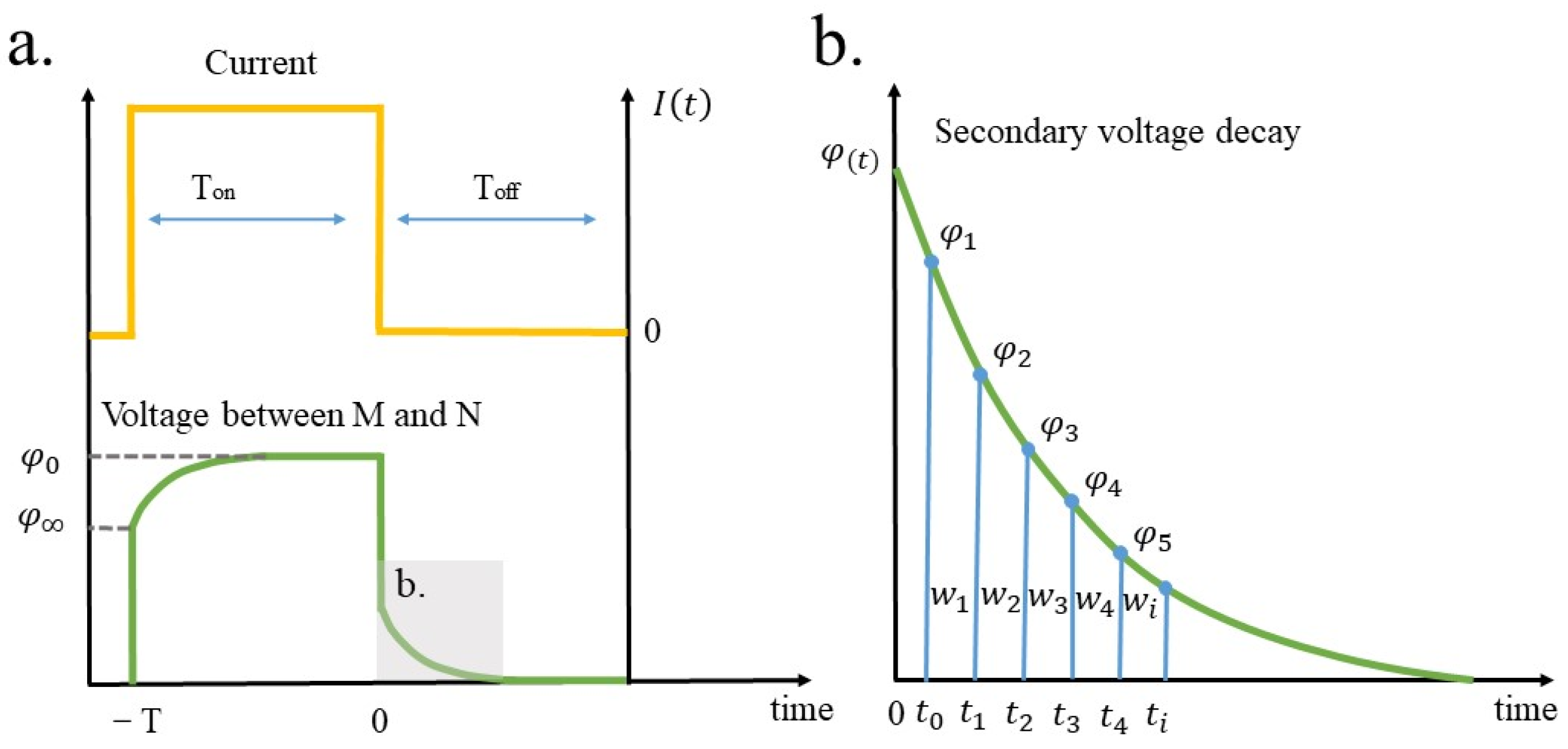
2.3. Induced Polarization Method
2.4. The Integrated Analysis of IP and SP Results
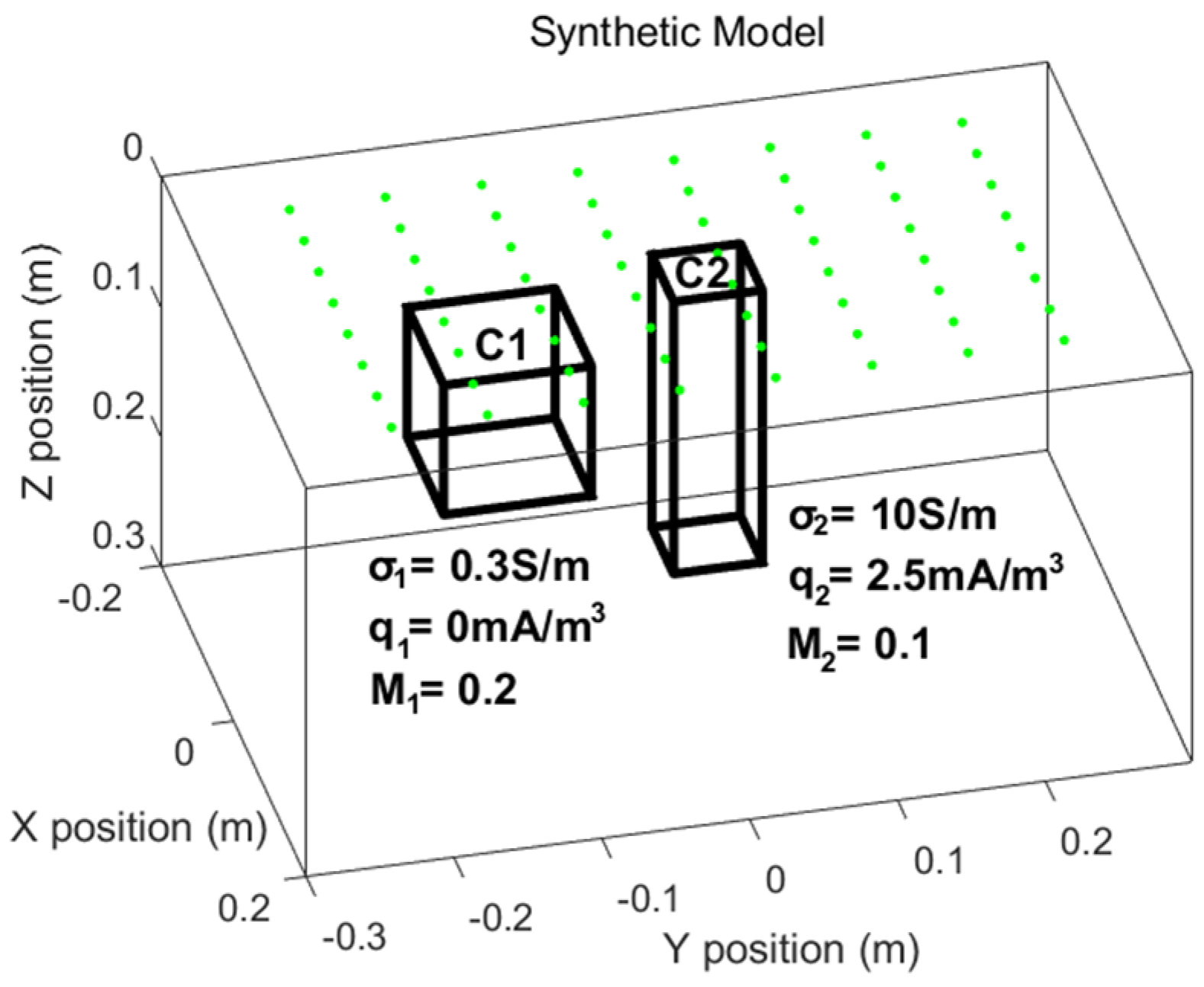
3. Synthetic Test
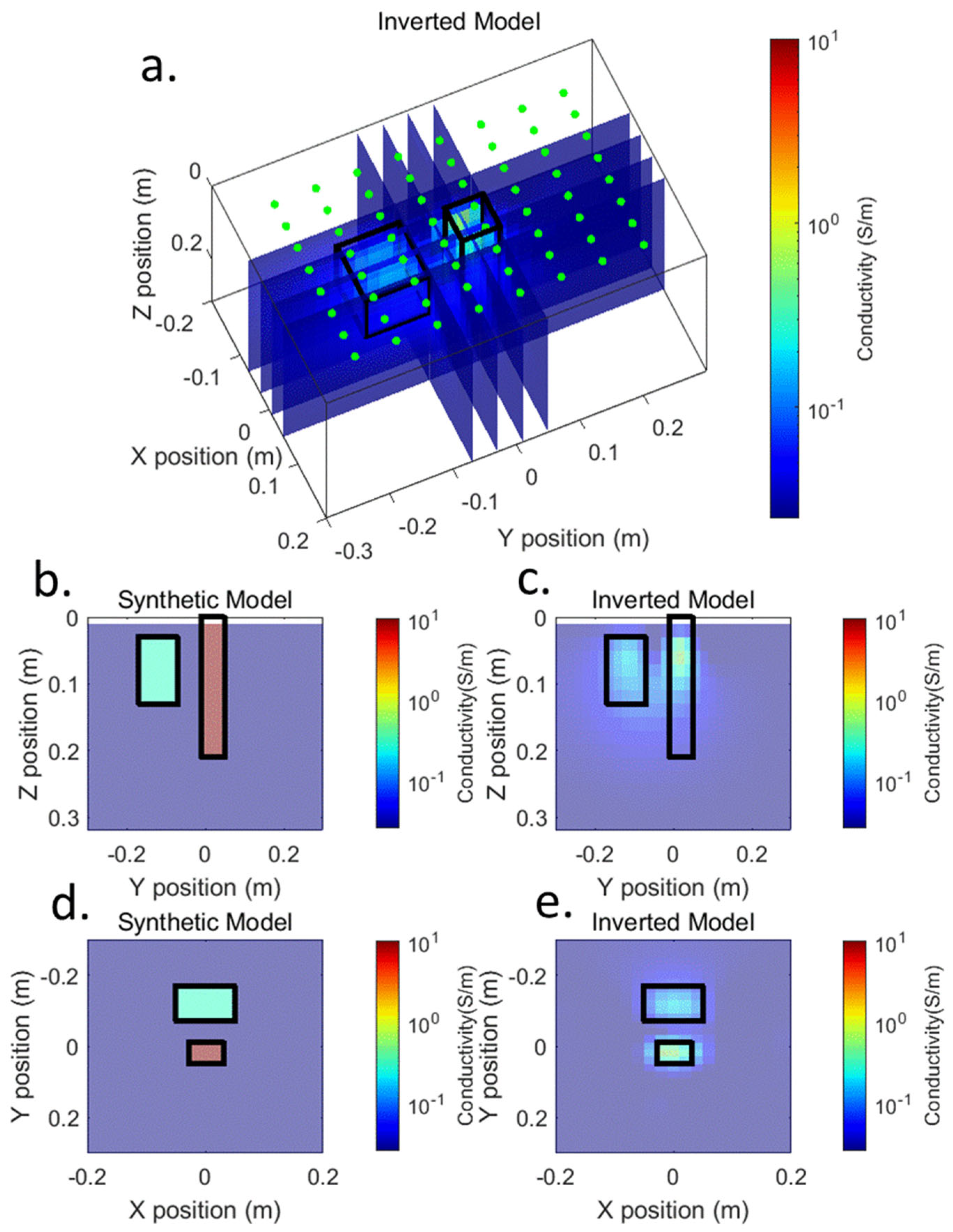
3.1. ERT
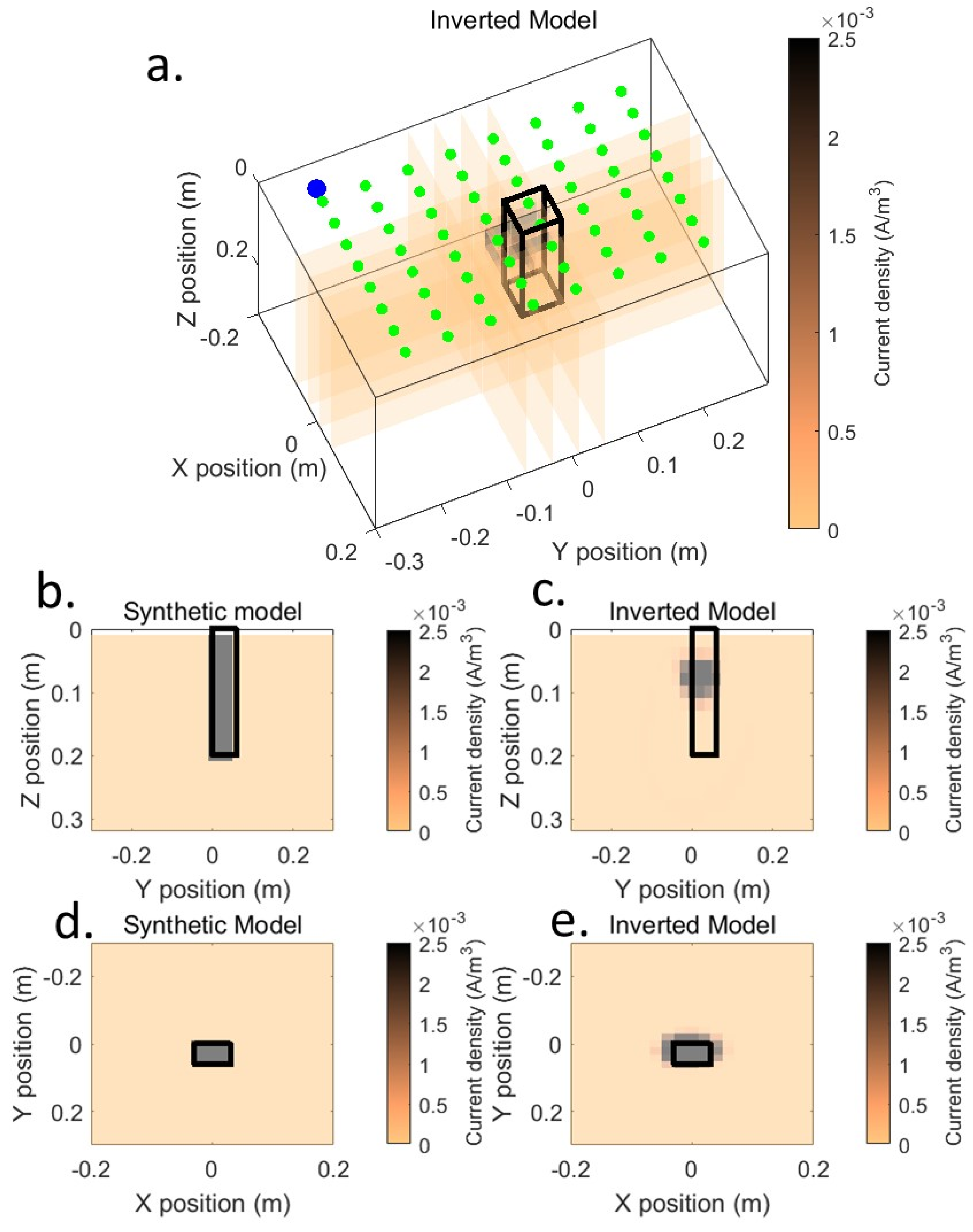
3.2. IP Inversion
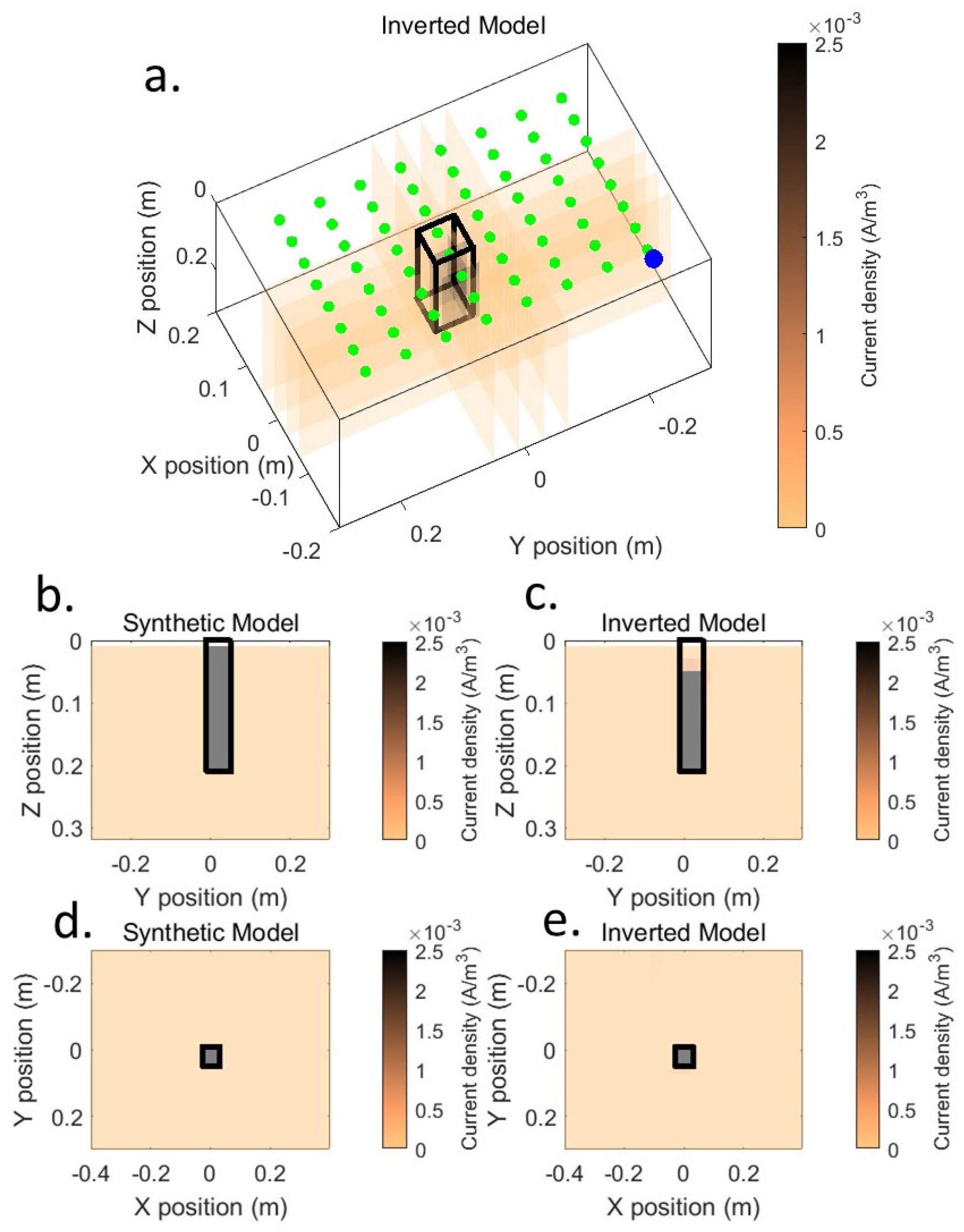
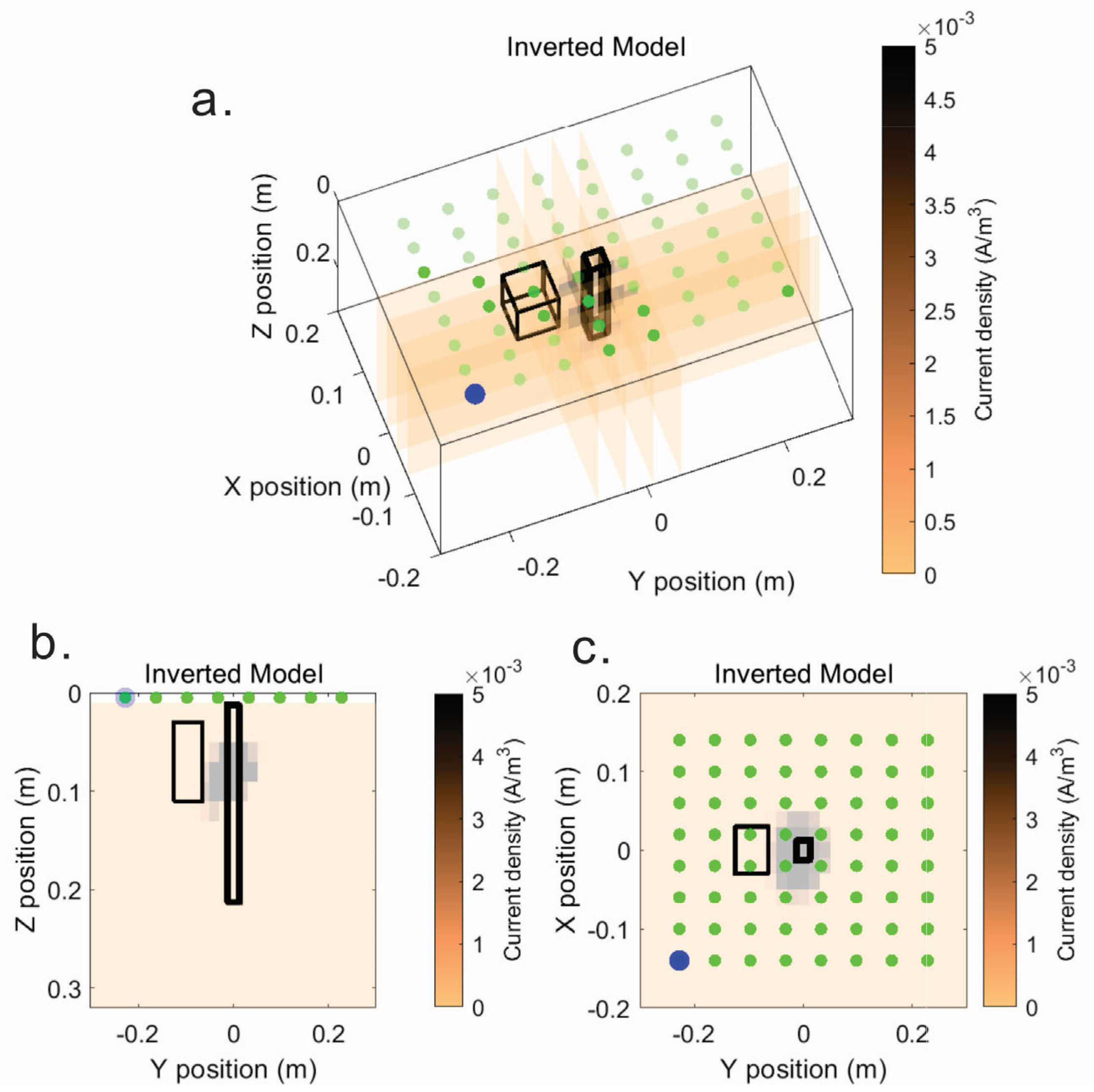
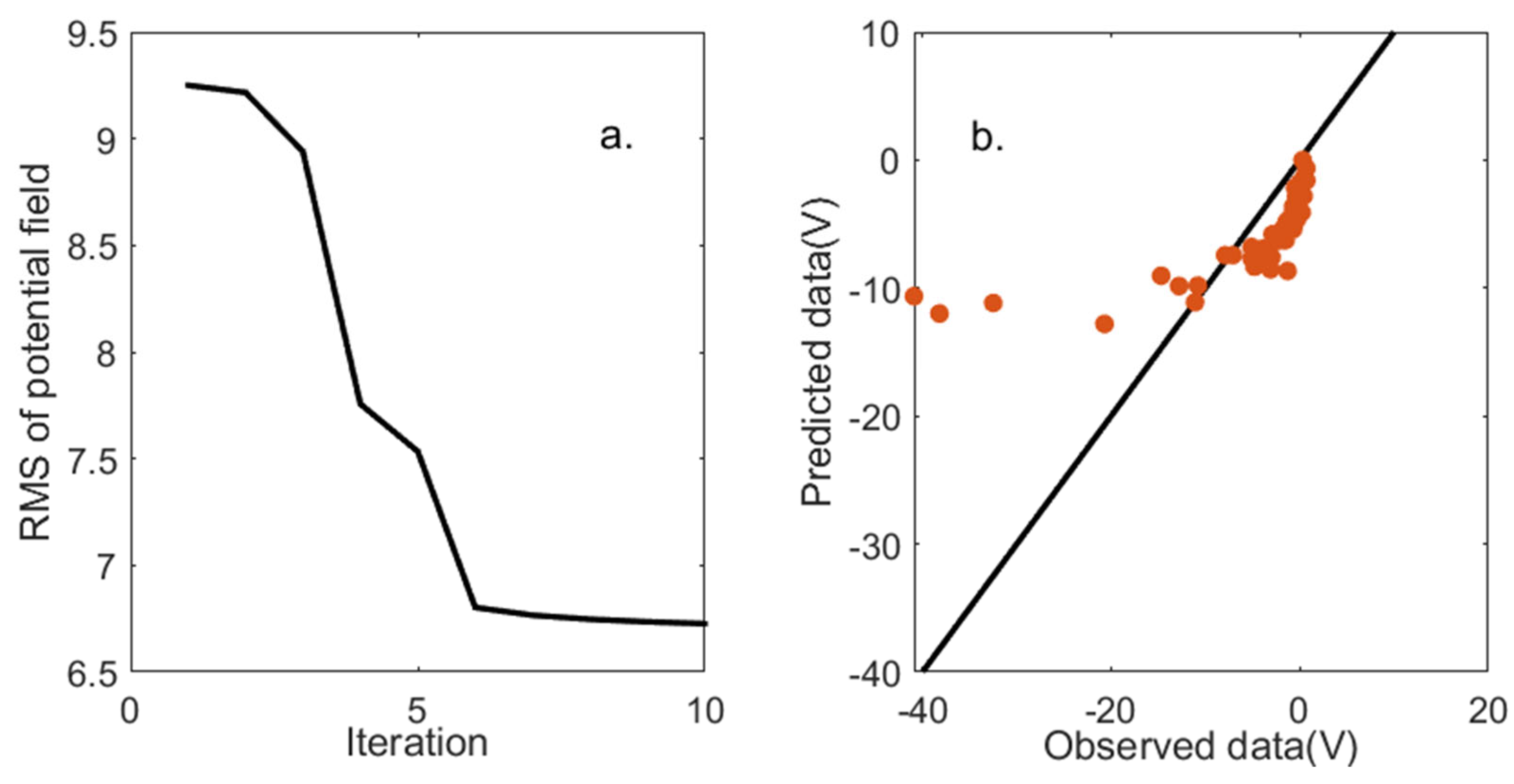
3.3. SP Inversion
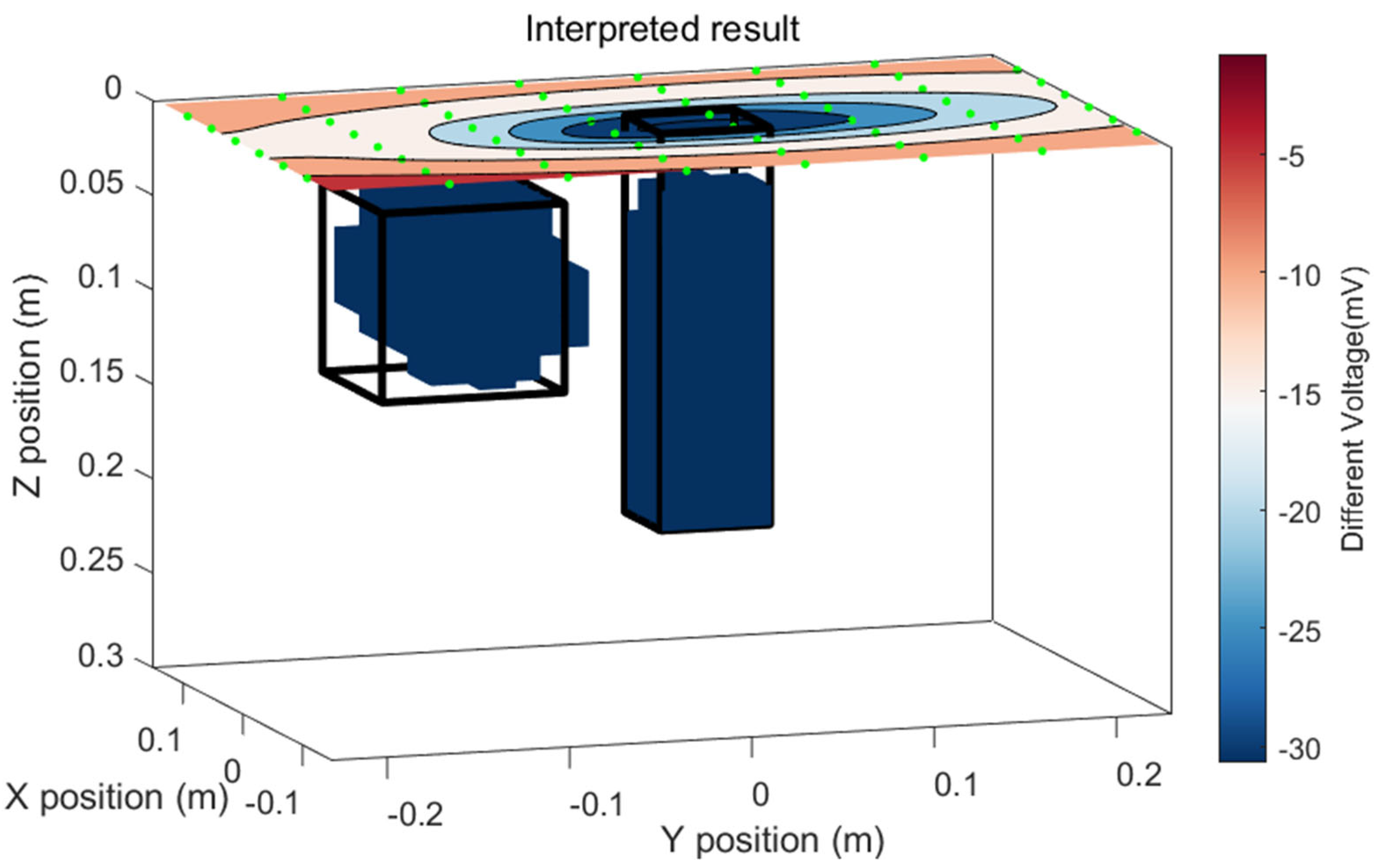
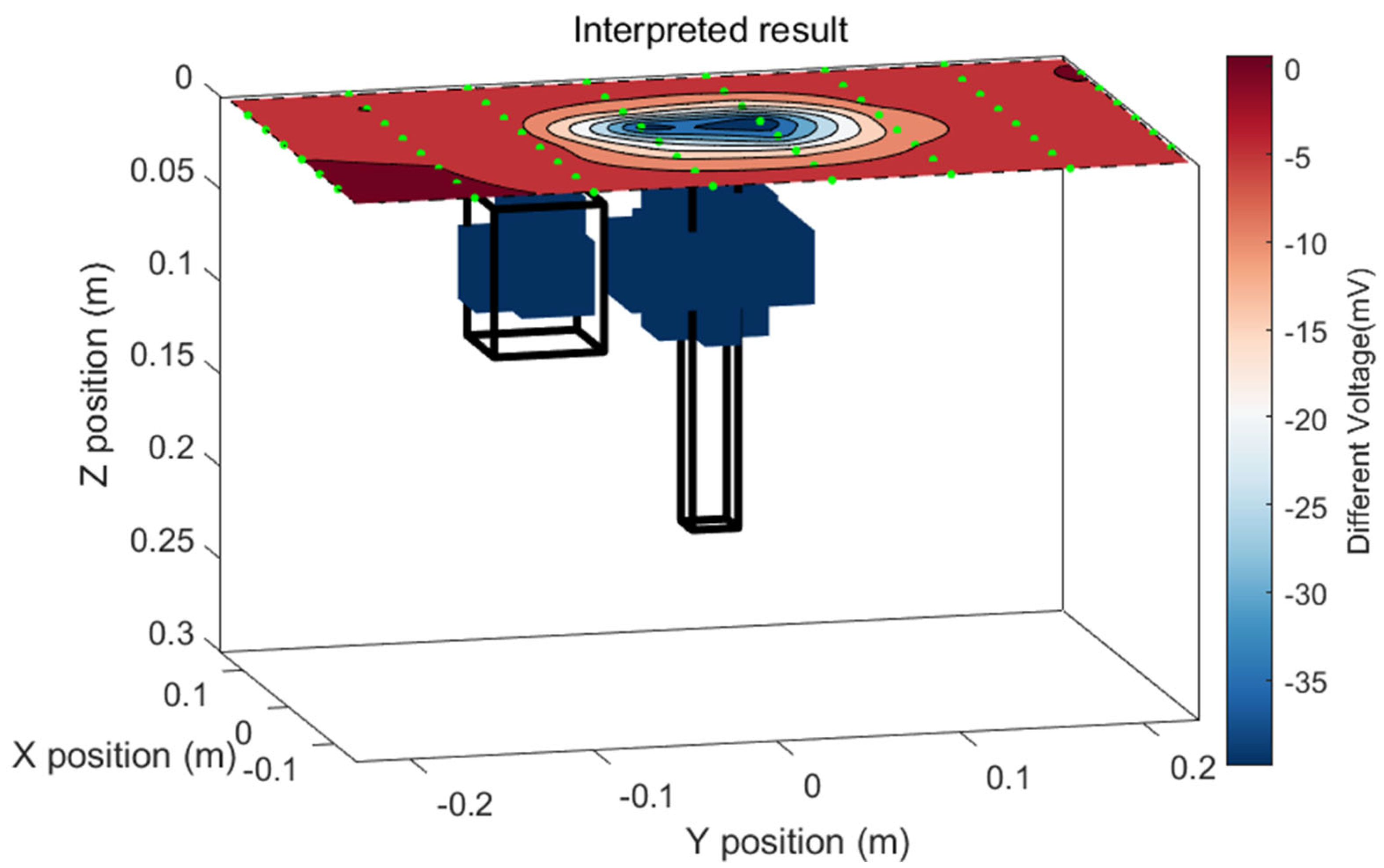
3.4. Integrated Result
4. Sandbox Experiment
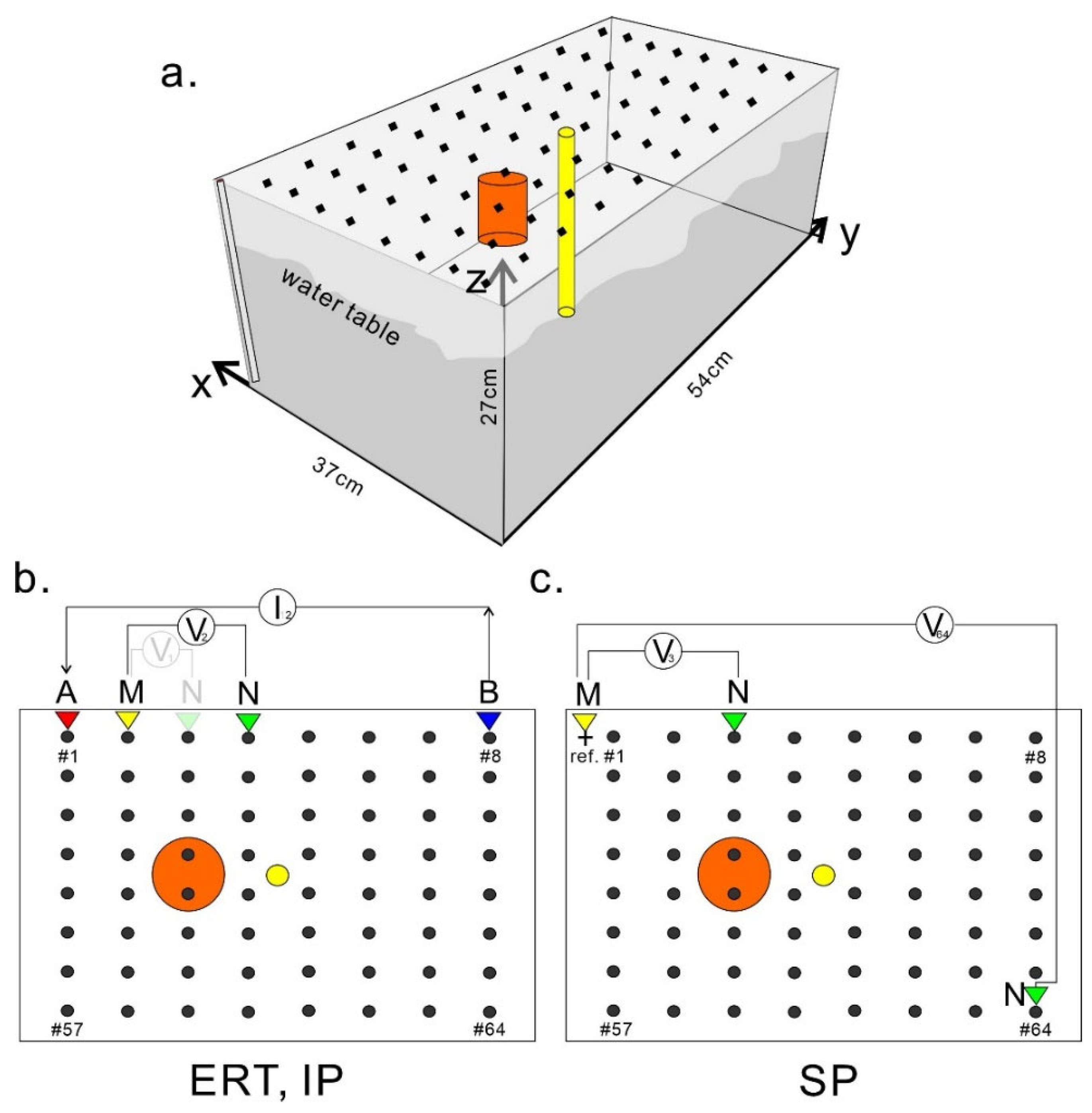
4.1. Experimental Setup
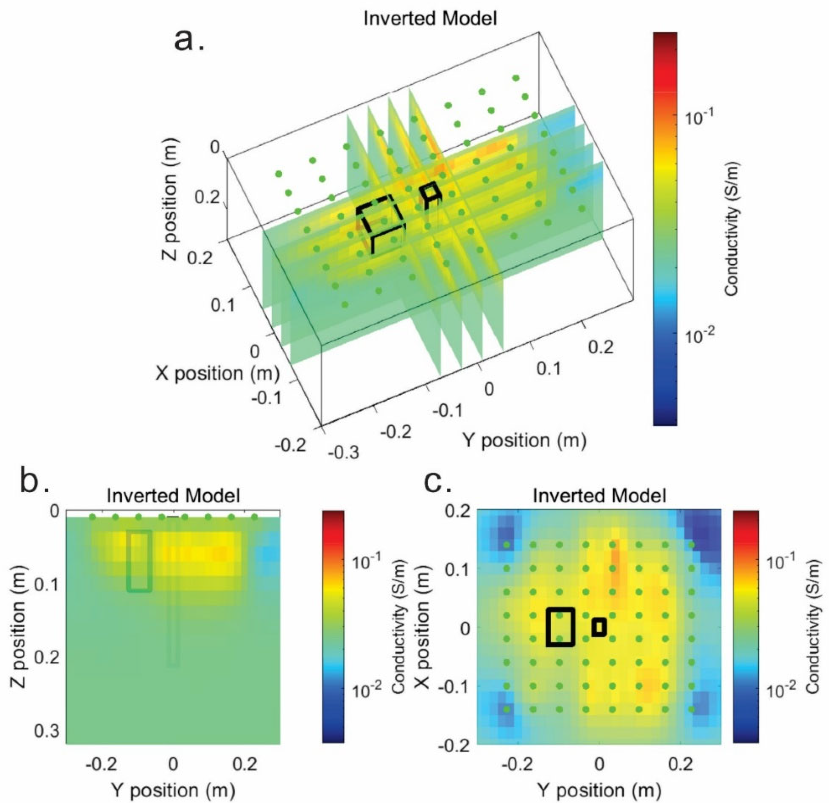
4.2. ERT
4.3. IP Inversion
4.4. SP Inversion
4.5. Integrated Result
5. Conclusions
Author Contributions
Funding
Data Availability Statement
Acknowledgments
Conflicts of Interest
Appendix A
Appendix B
References
- Okada, K. Breakthrough technologies for mineral exploration. Miner. Econ. 2022, 35, 429–454. [Google Scholar] [CrossRef]
- Schodde, R. Recent trends in gold discovery. In Proceedings of the 2011 NewGenGold Conference, Perth, Australia, 22–23 November 2011; Volume 2, pp. 1–19. [Google Scholar]
- Witherly, K. The evolution of minerals exploration over 60 years and the imperative to explore undercover. Lead. Edge 2012, 31, 292–295. [Google Scholar] [CrossRef]
- Eaton, D.W.; Milkereit, B.; Salisbury, M. Seismic methods for deep mineral exploration: Mature technologies adapted to new targets. Lead. Edge 2003, 22, 580–585. [Google Scholar] [CrossRef]
- Malehmir, A.; Durrheim, R.; Bellefleur, G.; Urosevic, M.; Juhlin, C.; White, D.J.; Milkereit, B.; Campbell, G. Seismic methods in mineral exploration and mine planning: A general overview of past and present case histories and a look into the future. Geophysics 2012, 77, WC173–WC190. [Google Scholar] [CrossRef]
- Witherly, K.; Irvine, R.; Morrison, E.B. The Geotech VTEM time domain helicopter EM system. In SEG Technical Program Expanded Abstracts; SEG: Denver, CO, USA, 2004; pp. 1217–1220. [Google Scholar]
- Sorensen, K.I.; Auken, E. SkyTEM—A New High-resolution Helicopter Transient Electromagnetic System. Explor. Geophys. 2004, 35, 194–202. [Google Scholar] [CrossRef]
- Smith, R.S.; Hodges, G.; Lemieux, J. Case histories illustrating the characteristics of the HeliGEOTEM system. Explor. Geophys. 2009, 40, 246–256. [Google Scholar] [CrossRef]
- Konieczny, G.; Smiarowski, A.; Miles, P. Breaking through the 25/30 Hz barrier: Lowering the base frequency of the HELITEM airborne EM system. In SEG Technical Program Expanded Abstracts; SEG: Denver, CO, USA, 2016; pp. 2218–2222. [Google Scholar]
- Evans, R.L. A seafloor gravity profile across the TAG Hydrothermal Mound. Geophys. Res. Lett. 1996, 23, 3447–3450. [Google Scholar] [CrossRef]
- Dransfield, M.; Milkereit, B. Airborne Gravity Gradiometry in the Search for Mineral Deposits. In Proceedings of the Exploration 07: Fifth Decennial International Conference on Mineral Exploration, Toronto, ON, Canada, 9–12 September 2007. [Google Scholar]
- Martinez, C.; Li, Y.; Krahenbuhl, R.; Braga, M.A. 3D inversion of airborne gravity gradiometry data in mineral exploration: A case study in the Quadrilátero Ferrífero, Brazil. Geophysics 2013, 78, B1–B11. [Google Scholar] [CrossRef]
- Gunn, P.; Dentith, M. Magnetic responses associated with mineral deposits. J. Aust. Geol. Geophys. 1997, 17, 145–158. [Google Scholar]
- Nabighian, M.N.; Grauch, V.J.S.; Hansen, R.O.; LaFehr, T.R.; Li, Y.; Peirce, J.W.; Phillips, J.D.; Ruder, M.E. The historical development of the magnetic method in exploration. Geophysics 2005, 70, 33ND–61ND. [Google Scholar] [CrossRef]
- Galley, C.; Lelièvre, P.; Haroon, A.; Graber, S.; Jamieson, J.; Szitkar, F.; Yeo, I.; Farquharson, C.; Petersen, S.; Evans, R. Magnetic and Gravity Surface Geometry Inverse Modeling of the TAG Active Mound. J. Geophys. Res. Solid Earth 2021, 126, e2021JB022228. [Google Scholar] [CrossRef]
- Harris, A.C. Exploration and Discovery of Base-and Precious-Metal Deposits in the Circum-Pacific Region—A 2010 Perspective. Econ. Geol. 2012, 107, 1073–1074. [Google Scholar] [CrossRef]
- Loke, M.H. Electrical Imaging Surveys for Environmental and Engineering Studies, A Practical Guide to 2-D and 3-D Survey. 1999. Volume 70. Available online: https://pages.mtu.edu/~ctyoung/LOKENOTE.PDF (accessed on 15 June 2023).
- Chambers, J.E.; Kuras, O.; Meldrum, P.I.; Ogilvy, R.D.; Hollands, J. Electrical resistivity tomography applied to geologic, hydrogeologic, and engineering investigations at a former waste-disposal site. Geophysics 2006, 71, B231–B239. [Google Scholar] [CrossRef]
- Abu Rajab, J.S.; El-Naqa, A.R. Mapping groundwater salinization using transient electromagnetic and direct current resistivity methods in Azraq Basin, Jordan. Geophysics 2013, 78, B89–B101. [Google Scholar] [CrossRef]
- Zhang, G.; Zhang, G.-B.; Chen, C.-C.; Jia, Z.-Y. Research on Inversion Resolution for ERT Data and Applications for Mineral Exploration. Terr. Atmos. Ocean 2015, 26, 515–526. [Google Scholar] [CrossRef]
- Schoor, M.V. The application of in-mine electrical resistance tomography (ERT) for mapping potholes and other disruptive features ahead of mining. J. S. Afr. Inst. Min. Metall. 2005, 105, 447–451. [Google Scholar]
- Giao, P.; Chung, S.; Kim, D.; Tanaka, H. Electric imaging and laboratory resistivity testing for geotechnical investigation of Pusan clay deposits. J. Appl. Geophys. 2003, 52, 157–175. [Google Scholar] [CrossRef]
- Perrone, A.; Lapenna, V.; Piscitelli, S. Electrical resistivity tomography technique for landslide investigation: A review. Earth-Sci. Rev. 2014, 135, 65–82. [Google Scholar] [CrossRef]
- Goto, T.N.; Takekawa, J.; Mikada, H.; Kasaya, T.; Machiyama, H.; Iijima, K.; Sayanagi, K. Resistivity survey of seafloor massive sulfide areas in the Iheya north area, off Okinawa, Japan. In Proceedings of the 11th SEGJ International Symposium, Yokohama, Japan, 18–21 November 2013; pp. 298–301. [Google Scholar]
- Park, J.-O.; You, Y.-J.; Kim, H.J. Electrical resistivity surveys for gold-bearing veins in the Yongjang mine, Korea. J. Geophys. Eng. 2009, 6, 73–81. [Google Scholar] [CrossRef]
- Batista-Rodríguez, J.A.; Pérez-Flores, M.A. Contribution of ERT on the Study of Ag-Pb-Zn, Fluorite, and Barite Deposits in Northeast Mexico. Minerals 2021, 11, 249. [Google Scholar] [CrossRef]
- Ishizu, K.; Goto, T.; Ohta, Y.; Kasaya, T.; Iwamoto, H.; Vachiratienchai, C.; Siripunvaraporn, W.; Tsuji, T.; Kumagai, H.; Koike, K. Internal structure of a seafloor massive sulfide deposit by electrical resistivity tomography, Okinawa Trough. Geophys. Res. Lett. 2019, 46, 11025–11034. [Google Scholar] [CrossRef]
- Revil, A.; Florsch, N.; Mao, D. Induced polarization response of porous media with metallic particles—Part 1: A theory for disseminated semiconductors. Geophysics 2015, 80, D525–D538. [Google Scholar] [CrossRef]
- Revil, A.; Abdel Aal, G.Z.; Atekwana, E.A.; Mao, D.; Florsch, N. Induced polarization response of porous media with metallic particles—Part 2: Comparison with a broad database of experimental data. Geophysics 2015, 80, D539–D552. [Google Scholar] [CrossRef]
- Mao, D.; Revil, A. Induced polarization response of porous media with metallic particles—Part 3: A new approach to time-domain induced polarization tomography. Geophysics 2016, 81, D345–D357. [Google Scholar] [CrossRef]
- Mao, D.; Revil, A.; Hinton, J. Induced polarization response of porous media with metallic particles—Part 4: Detection of metallic and nonmetallic targets in time-domain induced polarization tomography. Geophysics 2016, 81, D359–D375. [Google Scholar] [CrossRef]
- Schlumberger, C. Etude sur la Prospection Electrique du Sous-Sol.; Gauthier-Villars: Paris, France, 1920. [Google Scholar]
- Revil, A.; Vaudelet, P.; Su, Z.; Chen, R. Induced Polarization as a Tool to Assess Mineral Deposits: A Review. Minerals 2022, 12, 571. [Google Scholar] [CrossRef]
- Hallof, P.; Yamashita, M.; Fink, J.; Sternburg, B.; McAlister, E.; Wieduwilt, W. The use of the IP method to locate gold-bearing sulfide mineralization. In Induced Polarization Applications and Case Histories; Society of Exploration Geophysicists: Houston, TX, USA, 1990. [Google Scholar]
- Florsch, N.; Llubes, M.; Téreygeol, F.; Ghorbani, A.; Roblet, P. Quantification of slag heap volumes and masses through the use of induced polarization: Application to the Castel-Minier site. J. Archaeol. Sci. 2011, 38, 438–451. [Google Scholar] [CrossRef]
- Sumner, J.S. Principles of Induced Polarization for Geophysical Exploration; Elsevier: Amsterdam, The Netherlands, 2012. [Google Scholar]
- Günther, T.; Martin, T. Spectral two-dimensional inversion of frequency-domain induced polarization data from a mining slag heap. J. Appl. Geophys. 2016, 135, 436–448. [Google Scholar] [CrossRef]
- Liu, W.; Chen, R.; Cai, H.; Luo, W. Robust statistical methods for impulse noise suppressing of spread spectrum induced polarization data, with application to a mine site, Gansu province, China. J. Appl. Geophys. 2016, 135, 397–407. [Google Scholar] [CrossRef]
- Anderson, L.A.; Keller, G.V. A study in induced polarization. Geophysics 1964, 29, 848–864. [Google Scholar] [CrossRef]
- Revil, A.; Jardani, A. The Self-Potential Method: Theory and Applications in Environmental Geosciences; Cambridge University Press: Cambridge, UK, 2013. [Google Scholar]
- Grech, R.; Cassar, T.; Muscat, J.; Camilleri, K.P.; Fabri, S.G.; Zervakis, M.; Xanthopoulos, P.; Sakkalis, V.; Vanrumste, B. Review on solving the inverse problem in EEG source analysis. J. NeuroEng. Rehabil. 2008, 5, 25. [Google Scholar] [CrossRef] [PubMed]
- Michel, C.M.; Murray, M.M.; Lantz, G.; Gonzalez, S.; Spinelli, L.; Grave de Peralta, R. EEG source imaging. Clin. Neurophysiol. 2004, 115, 2195–2222. [Google Scholar] [CrossRef] [PubMed]
- Britton, J.W.; Frey, L.C.; Hopp, J.L.; Korb, P.; Koubeissi, M.Z.; Lievens, W.E.; Pestana-Knight, E.M.; St Louis, E.K. Electroencephalography (EEG): An Introductory Text and Atlas of Normal and Abnormal Findings in Adults, Children, and Infants; American Epilepsy Society: Chicago, IL, USA, 2016. [Google Scholar]
- Jardani, A.; Revil, A.; Bolève, A.; Dupont, J.P. Three-dimensional inversion of self-potential data used to constrain the pattern of groundwater flow in geothermal fields. J. Geophys. Res. Solid Earth 2008, 113. [Google Scholar] [CrossRef]
- Sato, M.; Mooney, H.M. The electrochemical mechanism of sulfide self-potentials. Geophysics 1960, 25, 226–249. [Google Scholar] [CrossRef]
- Heritiana, A.R.; Riva, R.; Ralay, R.; Boni, R. Evaluation of flake graphite ore using self-potential (SP), electrical resistivity tomography (ERT) and induced polarization (IP) methods in east coast of Madagascar. J. Appl. Geophys. 2019, 169, 134–141. [Google Scholar] [CrossRef]
- Embeng, S.B.N.; Meying, A.; Ndougsa-Mbarga, T.; Moreira, C.A.; Amougou, O.U.O. Delineation and Quasi-3D Modeling of Gold Mineralization Using Self-Potential (SP), Electrical Resistivity Tomography (ERT), and Induced Polarization (IP) Methods in Yassa Village, Adamawa, Cameroon: A Case Study. Pure Appl. Geophys. 2022, 179, 795–815. [Google Scholar] [CrossRef]
- Shao, P.; Shang, Y.; Hasan, M.; Yi, X.; Meng, H. Integration of ERT, IP and SP methods in hard rock engineering. Appl. Sci. 2021, 11, 10752. [Google Scholar] [CrossRef]
- Kasaya, T.; Iwamoto, H.; Kawada, Y.; Hyakudome, T. Marine DC resistivity and self-potential survey in the hydrothermal deposit areas using multiple AUVs and ASV. Terr. Atmos. Ocean. Sci. 2020, 31, 5. [Google Scholar] [CrossRef]
- Zhu, Z.; Tao, C.; Shen, J.; Revil, A.; Deng, X.; Liao, S.; Zhou, J.; Wang, W.; Nie, Z.; Yu, J. Self-potential tomography of a deep-sea polymetallic sulfide deposit on Southwest Indian Ridge. J. Geophys. Res. Solid Earth 2020, 125, e2020JB019738. [Google Scholar] [CrossRef]
- Su, Z.; Tao, C.; Shen, J.; Revil, A.; Zhu, Z.; Deng, X.; Nie, Z.; Li, Q.; Liu, L.; Wu, T. 3D self-potential tomography of seafloor massive sulfide deposits using an autonomous underwater vehicle. Geophysics 2022, 87, B255–B267. [Google Scholar] [CrossRef]
- Kawada, Y.; Kasaya, T. Marine self-potential survey for exploring seafloor hydrothermal ore deposits. Sci. Rep. 2017, 7, 13552. [Google Scholar] [CrossRef]
- Mendonça, C.A. Forward and inverse self-potential modeling in mineral exploration. Geophysics 2008, 73, F33–F43. [Google Scholar] [CrossRef]
- Oldenburg, D.W.; Li, Y. Inversion for applied geophysics: A tutorial. In Near-Surface Geophysics; Butler, D.K., Ed.; No.13 in Investigations in Geophysics; SEG: Tulsa, OK, USA, 2023; Chap 5; pp. 89–150. [Google Scholar]
- Sill, W.R. Self-potential modeling from primary flows. Geophysics 1983, 48, 76–86. [Google Scholar] [CrossRef]
- Rittgers, J.B.; Revil, A.; Karaoulis, M.; Mooney, M.A.; Slater, L.D.; Atekwana, E.A. Self-potential signals generated by the corrosion of buried metallic objects with application to contaminant plumes. Geophysics 2013, 78, EN65–EN82. [Google Scholar] [CrossRef]
- Amestoy, P.R.; Duff, I.S.; L’excellent, J.-Y.; Li, X.S. Analysis and comparison of two general sparse solvers for distributed memory computers. ACM Trans. Math. Softw. 2001, 27, 388–421. [Google Scholar] [CrossRef]
- Amestoy, P.R.; Guermouche, A.; L’Excellent, J.-Y.; Pralet, S. Hybrid scheduling for the parallel solution of linear systems. Parallel Comput. 2006, 32, 136–156. [Google Scholar] [CrossRef]
- Revil, A.; Karaoulis, M.; Srivastava, S.; Byrdina, S. Thermoelectric self-potential and resistivity data localize the burning front of underground coal fires. Geophysics 2013, 78, B259–B273. [Google Scholar] [CrossRef]
- Su, Z.; Tao, C.; Zhu, Z.; Revil, A.; Shen, J.; Nie, Z.; Li, Q.; Deng, X.; Zhou, J.; Liu, L. Joint Interpretation of Marine Self-Potential and Transient Electromagnetic Survey for Seafloor Massive Sulfide (SMS) Deposits: Application at TAG Hydrothermal Mound, Mid-Atlantic Ridge. J. Geophys. Res. Solid Earth 2022, 127, e2022JB024496. [Google Scholar] [CrossRef]
- Patella, D. Self-potential global tomography including topographic effects. Geophys. Prospect. 1997, 45, 843–863. [Google Scholar] [CrossRef]
- Minsley, B.J.; Sogade, J.; Morgan, F.D. Three-dimensional source inversion of self-potential data. J. Geophys. Res. 2007, 112. [Google Scholar] [CrossRef]
- Hansen, P.C.; O’Leary, D.P. The Use of the L-Curve in the Regularization of Discrete Ill-Posed Problems. SIAM J. Sci. Comput. 1993, 14, 1487–1503. (In English) [Google Scholar] [CrossRef]
- Last, B.J.; Kubik, K. Compact gravity inversion. Geophysics 1983, 48, 713–721. [Google Scholar] [CrossRef]
- Zhdanov, M.S.; Ekaterina, T. Minimum support nonlinear parametrization in the solution of a 3D magnetotelluric inverse problem. Inverse. Probl. 2004, 20, 937. [Google Scholar] [CrossRef]
- Pidlisecky, A.; Haber, E.; Knight, R. RESINVM3D: A 3D resistivity inversion package. Geophysics 2007, 72, H1–H10. [Google Scholar] [CrossRef]
- Haber, E. Computational Methods in Geophysical Electromagnetics; Mathematics in Industry Series; Society for Industrial and Applied Mathematics: Philadelphia, PA, USA, 2014. [Google Scholar]
- Slater, L.D.; Lesmes, D. IP interpretation in environmental investigations. Geophysics 2002, 67, 77–88. [Google Scholar] [CrossRef]
- Florsch, N.; Llubes, M.; Téreygeol, F. Induced polarization 3D tomography of an archaeological direct reduction slag heap. Near Surf. Geophys. 2012, 10, 567–574. [Google Scholar] [CrossRef]
- Oldenburg, D.W.; Li, Y. Inversion of induced polarization data. Geophysics 1994, 59, 1327–1341. [Google Scholar] [CrossRef]


Disclaimer/Publisher’s Note: The statements, opinions and data contained in all publications are solely those of the individual author(s) and contributor(s) and not of MDPI and/or the editor(s). MDPI and/or the editor(s) disclaim responsibility for any injury to people or property resulting from any ideas, methods, instructions or products referred to in the content. |
© 2023 by the authors. Licensee MDPI, Basel, Switzerland. This article is an open access article distributed under the terms and conditions of the Creative Commons Attribution (CC BY) license (https://creativecommons.org/licenses/by/4.0/).
Share and Cite
Su, Z.; Revil, A.; Ghorbani, A.; Zhang, X.; Zhao, X.; Richard, J. Combining Electrical Resistivity, Induced Polarization, and Self-Potential for a Better Detection of Ore Bodies. Minerals 2024, 14, 12. https://doi.org/10.3390/min14010012
Su Z, Revil A, Ghorbani A, Zhang X, Zhao X, Richard J. Combining Electrical Resistivity, Induced Polarization, and Self-Potential for a Better Detection of Ore Bodies. Minerals. 2024; 14(1):12. https://doi.org/10.3390/min14010012
Chicago/Turabian StyleSu, Zhaoyang, André Revil, Ahmad Ghorbani, Xin Zhang, Xiang Zhao, and Jessy Richard. 2024. "Combining Electrical Resistivity, Induced Polarization, and Self-Potential for a Better Detection of Ore Bodies" Minerals 14, no. 1: 12. https://doi.org/10.3390/min14010012
APA StyleSu, Z., Revil, A., Ghorbani, A., Zhang, X., Zhao, X., & Richard, J. (2024). Combining Electrical Resistivity, Induced Polarization, and Self-Potential for a Better Detection of Ore Bodies. Minerals, 14(1), 12. https://doi.org/10.3390/min14010012