Abstract
Mineral resources are of great significance in the development of the national economy. Prospecting and forecasting are the key to ensure the security of mineral resources supply, promote economic development, and maintain social stability. The methods for prospecting prediction have evolved from qualitative to quantitative prediction, from empirical research to mathematical analysis. In recent years, deep learning algorithms have gradually entered the attention of geologists due to their robust learning and simulation ability in the application of prospecting prediction. Deep learning algorithms can effectively analyze and predict data, which have great significance in improving the efficiency and accuracy of mineral exploration. However, there are not many specific examples of their application in mineral exploration prediction, and researchers have not yet conducted a comprehensive discussion on the advantages, disadvantages, and accuracy of deep learning algorithms in mineral prospectivity mapping applications. This paper reviews and discusses the application of deep learning in prospecting prediction, highlighting the challenges faced by deep learning in the application of prospecting prediction in data preprocessing, data enhancement, system parameter adjustment, and accuracy evaluation, and puts forward specific suggestions for research in these aspects. The purpose of this paper is to provide a reference for the application of deep learning to researchers and practitioners in the field of prospecting prediction.
1. Introduction
Mineral resources are the cornerstone of modern social and economic development and are of great significance at the level of national strategic security. With the deepening of mineral exploitation and the gradual formation of world trade barriers, the deep prospecting prediction and exploration of strategic and pillar minerals have gradually become the focus of attention of various countries and government agencies. As a technical means of comprehensive utilization of geological, geophysical, geochemical, and other multi-source information, mineral prediction mapping can effectively identify areas with mineral resource potential, so as to guide exploration activities, improve exploration efficiency, and reduce costs.
The formation of the deposit is a long and complex process, which is influenced by many factors. The basic geological information of the study area, such as geological structure background, lithology characteristics, mineral types, alteration characteristics of surrounding rock, geophysical and geochemical anomalies, and prospecting engineering data, are the basis of prospecting and prediction research. The prediction of mineral resources is supported by the theory of geological mineralization, and the comprehensive analysis of the mineral geological data accumulated in geological survey is carried out to summarize the metallogenic law and extract the metallogenic information, delineate the prospecting potential area, and predict the amount of resources [1,2]. Early prospecting prediction is mainly the prediction of the prospecting potential area or even target area, that is, metallogenic prediction, which mainly relies on metallogenic theory, the metallogenic system, comprehensive analysis of geological experience, and field geological survey to carry out qualitative evaluation. Since the purpose of geological work is to pursue the quantity and economic value of resources, the quantitative prediction method estimates the quantity, value, and origin of undiscovered mineral resources by showing the economic feasibility related to mineral resources, so the quantitative prospecting prediction becomes inevitable.
In 1976, the International Union of Earth Sciences put forward the standard quantitative method of resource prediction, and then with the wide application of geographic information systems, quantitative prediction began to develop in the direction of mathematical geology. Quantitative evaluation based on mathematical statistical models can process the data of complex statistical distribution characteristics, and can also explore the potential nonlinear relationship between large-scale high-dimensional mineralization information and ore deposits [3,4,5]. The model methods mainly include two types: one is a knowledge-driven model, which relies on subjective expert understanding, and combines experience with actual survey data to synthesize information and delineate prospective areas, which is suitable for areas with insufficient exploration data (Table 1) [6,7,8,9]. The American scholar Singer put forward the “three-part” metallogenic prediction method in 1993, emphasizing the comprehensive analysis of geologists’ subjective experience and mining area geological exploration data [10]. Zhao Pengda put forward three prediction theories of similarity analogy, difference seeking, and quantitative combined ore control in 1983 [11]. The second is the data-driven model [5,6,7,9], which is heavy on correlation and light on causation, and is suitable for further exploration in areas where there is already sufficient exploration data. Without considering the subjective factors brought by ore-forming theory and the ore-forming system, a mathematical model is established to predict mineral resources according to the relationship between various factors. The method of metallogenic prediction based on a knowledge-driven metallogenic model has great advantages in shallow surface and low geological exploration environments. However, with the large-scale exploitation of the earth’s shallow minerals, the exploration of hidden and deep deposits has gradually become the mainstream, the geological information has become extremely complex due to the influence of factors such as mixing, compounding, covering, and superposition [12], and the limitations of knowledge-driven methods have gradually emerged. Common prospecting prediction model algorithms mainly include statistical analysis methods such as the evidence weight method [13,14,15], information content method and regression analysis [16,17], traditional machine learning algorithms such as the support vector machine [6,18,19,20,21,22] and random forest [5,22,23,24,25], and deep learning algorithms represented by artificial neural networks, which provide an important theoretical basis for metallogenic prediction. Through the data-driven model, we can obtain the apparent or even hidden mineralization characteristics related to the formation of mineral resources from massive data, determine the deep relationship between ore-forming elements and mineralization, and help to optimize the existing ore-forming theory and prospecting technology. However, when dealing with complex geological data, the traditional method has some problems, such as the limitation of the data dimension, difficulty in feature selection, and low prediction accuracy. Therefore, further improving the accuracy and practicability of metallogenic prediction has become one of the difficulties in metallogenic prediction. In this context, deep learning, as a new technical means, has gradually attracted attention because of its ability to deal with complex relationships and nonlinear representation of high-dimensional data.

Table 1.
Comparison of several common metallogenic prediction methods.
Deep learning is characterized by continuous hierarchical representation learning and it can handle nonlinear representations of complex relationships [26,27]. Unlike traditional statistical methods, it does not require specific data distribution or independence assumptions, nor does it require in-depth study of deposit genesis or pre-analysis of geological feature correlations [22,28]. By mining the high-dimensional abstract features of various geological information, deep learning improves the comprehensive utilization rate of geoscience big data, makes the prediction results more intuitive and objective, and has great potential for processing nonlinear and high-dimensional earth science data [4,9,29]. Therefore, deep learning is a set of popular techniques for metallogenic prediction. At present, the algorithms used in the field of prospecting prediction mainly include the convolutional neural network, recurrent neural network, deep autoencoder, adversarial neural network, etc., which have been widely used in the fields of image and speech recognition. Among them, convolutional neural networks are the most widely used, including LeNet, AlexNet, VggNet, GoogleNet, ResNet, and other structures. The initial use of deep learning is for image recognition, and the data type of the remote sensing image is an image. Therefore, the remote sensing image has natural advantages as a data type of deep learning prospecting. In addition, geochemical data is one of the most widely used data types for deep learning. Xiong et al. [30] and Zuo et al. [31] successfully identified mineral-related geochemical anomalies by applying deep autoencoders to regional chemical data. Li et al. [32], Liu et al. [33,34], and Zheng et al. [35], respectively, used convolutional neural networks to make prospecting predictions in the study area and achieved good results. The application of deep learning algorithms in mineral prediction has made remarkable progress and achievements. Although there are still challenges in using point data to capture complex mineralization anomalies with spatial structure and high model complexity [36,37], its advantages in processing complex geological data and improving prediction accuracy make it an important direction for future mineral prediction research and application. According to previous studies, deep learning algorithms have been applied to various types of minerals such as Au, Fe, Cu, W-Sn, Pb-Zn, REE, etc., with good effect, and their future application prospects are very wide.
This paper aims to systematically review and summarize the latest research progress and application of deep learning in metallogenic prediction. And no one has ever concretely summarized the advantages and possible limitations of deep learning compared to other methods in mineral prospectivity mapping practice. By reviewing the current research results, methods, and cases, the application prospects and existing problems of deep learning technology in this field are discussed, helping researchers to understand the current research hotspots and future development direction, and providing references for research and application in related fields. The article’s structure is as follows. The first section mainly introduces the data types and data formats used by deep learning in the application of prospecting; the second section mainly introduces the main types of deep learning algorithm models; the third section introduces several application examples of deep learning in geological prospecting; the fourth section systematically summarizes the outstanding problems and future development trends of deep learning in the application of prospecting; and the fifth section concludes.
2. Data Foundation
2.1. Data Types
The types of data required for mineral prediction mapping mainly include geological data, geophysical data, geochemical data, remote sensing data, and so on. These data types play a crucial role in mineral prediction mapping and can help scientists and geological experts better understand and predict the location and type of mineral deposits. Geological data are the basis for mineral prospecting prediction, including information on petrology, mineralogy, ore deposit geology, and ore-forming structures. These data help determine geological structures and rock types, extract key geological information related to mineralization, delineate geological units as a basis for regional analogies, and thereby infer potential mineral deposit locations. Geophysical data are obtained by measuring changes in the Earth’s physical fields, such as gravity, magnetic force, and seismic wave data. These data can reveal differences in the density and elasticity of underground materials, providing a comprehensive assessment of the Earth’s physical field within a selected area, and thus helping to locate mineral deposits. Geochemical data are obtained by analyzing the chemical compositions of soil, water, and rocks. Abnormal concentrations of specific elements and compounds may indicate the presence of mineral deposits, and the anomaly zones are delineated through the integration of various types of geochemical data within the study area. Remote sensing data use satellite and aerial photography technology to obtain information about surface features, helping to identify surface cover and vegetation patterns, as well as alteration information related to mineralization, and delineate areas with key information for mineralization. MPM involves combining all the data anomalies to make mineral prospecting predictions within the study area.
The quality of the data we use has a significant impact on the results of our mineral prospecting predictions. Therefore, when selecting data, we should pay attention to the following issues:
- (1)
- Accuracy of data. The accuracy of data directly affects the credibility of data analysis and decision-making. If there are errors or biases in the data, it may lead to incorrect decision-making and analysis results.
- (2)
- Integrity of data. Collecting more complete data can lead to more accurate mineral deposit prediction, such as specific information about known mineral deposits.
- (3)
- Accuracy of data. In geological work, geological mapping, geophysical prospecting, geochemical prospecting, and remote sensing are all carried out at a certain scale. In practical work, the higher the precision and resolution, the more beneficial it is for predicting results.
- (4)
- The timeliness of data. As the times change and people’s perceptions evolve, some data may become outdated, so we need to regularly filter the data we collect.
2.2. Geological Database
2.2.1. Strata and Magmatic Rocks
Strata are closely related to ore deposits, and many ore deposits are formed in specific strata or stratigraphic combinations. The role of strata in the ore-forming process is as follows: (1) the migration channel of ore-forming fluid; (2) enrichment sites of ore-forming materials. In strata-controlled skarn deposits, ore-forming materials are deposited in the weak zone of strata, and the occurrence of ore bodies is often the same as that of strata. For example, the widely distributed strata-controlled skarn deposits, such as Dongguashan and Shizishan in Anhui Province, China, are preserved in the Silurian–Triassic strata, and the occurrence of ore bodies is controlled by strata [38,39]. The formation of some ore deposits is due to material exchange between strata and magmatic rocks, and ore-forming materials are enriched. At this time, strata closely related to ore-forming formations are also the characteristics that need to be paid attention to in prospecting and prediction. For example, the formation of the famous Huangshan magmatic copper–nickel sulfide deposit in the Central Asian orogenic belt is closely related to the Carboniferous and Jurassic strata [40,41]. For the sedimentary deposit, the strata are the ore-forming material itself, such as limestone, gypsum rock, and so on. The main geological information includes the mineralizing strata, ore-forming strata, controlling strata, rock texture and dip, mineral composition, geological age, distribution of igneous rocks, types of intrusive rocks, distribution of granite, control of mineralization by intrusive bodies, and so on. One of the limitations of geological data is that geological bodies are oriented in a certain way, and predicting in plain view is affected by the distribution of surface geological bodies.
Magmatic activity is closely related to the formation of ore deposits, and magmas provide the heat and some ore-forming materials needed for mineralization. Most magmatic deposits are directly related to magmatic rocks, such as the Bushveld magmatic Cu-Ni-PGE sulfide deposit in South Africa [42] and the Jinchuan Cu-Ni sulfide deposit in Gansu Province, China [43]. Their mineral sources and occurrence beds are located in magmatic rocks. Hydrothermal deposits are generally formed near the contact zone between magma and surrounding rock, such as the world-famous Cerro Verde super-large porphyry copper–molybdenum deposit in Peru [44] and the Mactung skarn schetungstate deposit in Canada [45].
2.2.2. Geological Structure
Geological structure is the most important ore-controlling factor at all scales from molecular to lithosphere [46]. The formation of mineral deposits is usually closely related to the tectonic framework, and the known large deposits in the world are often controlled by regional tectonic structures. The fluid flow and mineralization of the hydrothermal system are mainly controlled by the fault zone framework and its permeability structure [47]. From the perspective of the relationship between ore deposits and the tectonic environment, the distribution and occurrence of ore deposits and ore bodies usually have the following characteristics:
- Metallogenic magma and fluid often migrate along geological weak surfaces (fault plane, fold plane, shear zone, etc.);
- The structural plane (fault plane, fold plane, shear zone, etc.) is the main channel of heat source and the main place where heat exchange occurs;
- The repeated sliding of faults drives rapid changes in fluid pressure, velocity, and stress. When the induced fluid channel growth destroys the dynamic balance of the fluid system, the resulting rapid fluid depressor becomes the key driving factor for metal precipitation and mineralization [47];
- Metallogenic material precipitation often occurs in the weak structural plane and near the contact zone between the weak plane and the surrounding rock.
The location of ore deposits is often controlled by structural features. For example, the occurrence of the Withnell gold deposit in Australia is mainly controlled by the Mallina shear zone [48], and the formation of the Jiaodong gold deposit is mainly controlled by regional faults such as the Jiaojia Fault and Zhaoping Fault, which are formed in the extensional tectonic background [49].
The structure plays an important role in the formation of the deposit. With the increase in the distance from the tectonic plane, the fluidity of the fluid decreases, the heat loss increases, and the formation of the deposit becomes difficult. Therefore, the structure plays an important role in controlling and guiding the mineralization process, and the study of the structural characteristics is of great significance for prospecting and prediction. Structural information typically includes mineralizing structures, host structures, structures controlled by faults, folds, deep-seated faults, and so on. Like geological data, the defect of structural data is that structural surfaces have dips, and predicting in plain view is affected by the distribution of structures on the ground.
2.3. Geophysical Data
Geophysics is a comprehensive discipline that uses gravity exploration, magnetic exploration, electrical and electromagnetic exploration, seismic exploration, radioactive exploration, aerial geophysical exploration, and other methods to detect and analyze the material inside the Earth. Geophysical exploration provides detailed information of underground structure and material distribution, helps researchers to understand the deep dynamic process of mineralization and the crustal structure that determines the spatial distribution of ore deposits, reveals the spatial distribution of ore-forming and ore-controlling geological elements, and provides necessary intrinsic information for deep prospecting. The comprehensive application of a variety of geophysical methods provides a choice of method for the deep exploration of polymetallic deposits, and also plays a great role in the “transparency” of deep prospecting [50]. The geophysical method plays a particularly important role in the prospecting prediction of covered areas.
The theoretical basis of electrical exploration is the controlled factors of the electrical properties of rock (ore) or geological bodies, their action rules and IP effect [51], and the data types mainly include the numerical information of electrical conductivity and the dielectric property. When using resistivity data, it is necessary to select the resistivity interpretation chart with appropriate depth to reduce the error caused by the quality of the data itself. Magnetotelluric measurements of the resistivity of underground rocks can help identify conductive rock bands that may have mineralized prospects, and can also provide information about the depth and shape of conductive bands, but the magnetotelluric method is limited by itself, which may cause interference in the process of signal acquisition and processing. In addition, the electromagnetic method depends on natural field sources, whose strength and stability may affect the accuracy of data. The gravity data layer can provide valuable information about changes in rock density under a particular area, and can also provide information about the depth and thickness of the overlying sedimentary cover, and areas with thin sedimentary layers are more likely to have exposed rock units, which makes rock detection and sampling easier [52]. The aeromagnetic anomaly is usually regarded as one of the signs of mineralization, and it is necessary to process the raw data by the magnetic anomaly pole method to eliminate the dipolarity of the magnetic anomaly. Spectral gamma rays in aerial geophysical methods, due to their fast coverage and low unit area survey cost, can infer the concealed mineral and structural features related to mineral deposits, thus standing out from other geophysical methods [53,54].
The Victoria deposit in Sudbury, Canada was discovered by the inversion of various geophysical methods, despite decades of traditional geological work failing to uncover it [55]. Due to its location in the plains covered area, the syenite-type magnetite deposit discovered in recent years in the Qihe–Yucheng area of Shandong Province was also delimited by geophysical prospecting profiles, including magnetic prospecting and gravity prospecting, based on the abnormalities in the results of geophysical prospecting profile inversion [56]. Gold Potentiality Mapping of the Atalla Area and its environs in Egypt was established by the geological work combined with spectral gamma-ray data [53].
In summary, geophysical exploration plays an irreplaceable role in ore prospecting. Through reasonable selection and comprehensive application of different geophysical exploration methods, the underground ore body can be effectively identified and located, and the efficiency and success rate of ore prospecting can be improved. The study and application of geophysical data is of great significance to modern mineral resources exploration.
2.4. Geochemical Data
Geochemical data is the most common type of data used by researchers in geological survey and prospecting prediction. In the study of geological bodies and mineral resources, geochemical background and anomaly play a key role. The distribution map of geochemical data reflects the superposition field of geological bodies and mineral resources with different properties and grades [4,57].
Geochemical point data collected from stream sediments, lake sediments, soils, and rocks are important for discovering undiscovered deposits and monitoring environmental change [58]. In addition, geoelectrochemical survey is an unconventional comprehensive prospecting method to obtain geochemical information by geophysical means, which has a high application prospect in prospecting, especially in covering areas combined with other geological data [59,60,61,62]. In traditional research, the application of geochemical data is often based on the causal relationship between known mineralization and geochemical characteristics. However, due to the changes in geochemical data caused by water–rock reaction, weathering and denudation, and crustal movement, researchers may overlook the key role of some geochemical anomalies in mineralization [31,33].
In the 20th century, American geologists conducted geochemical surveys in the Carlin area of Nevada and found high anomaly zones of Au, As, Hg, Sb, and Ti, thus discovering and defining Carlin-type gold deposits [63]. The Hadamengou gold deposit in China was located by Au anomaly based on the geochemical survey of the 1:100,000 gold deposit area in Inner Mongolia, and the resources exceeded 100 tons [64].
In addition, in many areas with a high research degree, traditional logging data and geochemical logging data are abundant, these data can also be applied to geological-geophysical and geochemical exploration data according to their data types, and these data are also of great significance in data analysis [65,66]. However, it should also be noted that there are certain limitations to the earth chemical data from the data collection to the data processing and interpretation.
2.5. Remote Sensing Image Data
The appearance of remote sensing satellite technology makes the “space-air-ground” integrated monitoring become a reality, and provides a strong support for the exploration of mineral resources. Remote sensing images are widely used in the field of geological exploration for their convenience, speed, and economy. As a member of big data, remote sensing images are more and more applied in the prospecting work of the majority of scholars. Remote sensing satellites can provide a wide range of high-resolution image data. Through multispectral and hyperspectral imaging technology, spectral information of different bands can be captured, which helps to identify the mineral composition and characteristics of the surface; and especially important, remote sensing can efficiently and accurately detect altered minerals related to the hydrothermal process that formed the deposit [67,68]. In remote sensing data, spectral characteristics related to electronic vibration of different minerals are different, which brings convenience to mineral identification [69,70]. In addition, remote sensing satellites can regularly acquire image data of the same area, making dynamic monitoring possible. Compared to other data, remote sensing data can accurately identify mineralization anomalies, cover hard-to-reach areas, reduce costs, and improve efficiency.
The formation of mineral deposits is often accompanied by various forms of hydrothermal alteration, including magnetite alteration, pyritization, sericitization, sulphidization, carbonatization, chloritization, and so on. In practical applications of using remote sensing techniques for mineral deposit prediction, the extraction of hydrothermal alteration, especially OH-bearing minerals and iron oxides, is the most mainstream application method. Ali et al. [71] used ASTER, Advanced land imager, Landsat8, and Sentinel 2 datasets to identify hydrothermal alteration and delineate mineral prospecting areas in the eastern desert region of Egypt, which showed good consistency with the aeromagnetic, radiometric, and geochemical data. The Olympic Dam gold–copper–uranium deposit in Australia has not been well explored by geological and geophysical exploration methods, but great progress has been made after analyzing and comparing regional geological characteristics and geophysical data with remote sensing images. The mineralized area exceeds 20 km2 and the proved ore amount reaches 2 billion tons [72]. Dazhuyuan bauxite in the north Guizhou region is an important bauxite-producing area in China. Researchers used Landsat-8 and ASTER image data to analyze ground vegetation, rock strata distribution, rock types, and other information, which became an important means of bauxite exploration [73,74].
When using remote sensing data, in addition to paying attention to the resolution of the data, it is also important to choose data with less environmental interference, and it should be noted that the choice of information extraction method can lead to vastly different analysis results.
3. Deep Learning Technology
Deep learning refers to machine learning based on deep neural network models and methods, represented by an artificial neural network, and it can effectively identify the features and data types that have invisible associations with mineralization in mineral prediction, making up for the shortcomings of general machine learning algorithms [4]. The artificial neural network is an algorithmic mathematical model that mimics the behavior characteristics of biological neural networks to process complex data input with distributed and parallel information [75], and defines the variables in the network and their topological relationships in a structured way [34]. With the continuous development of deep learning, more and more deep learning algorithms are applied in prospecting prediction, which has become a hotspot and frontier of research. This paper uses “mineral prospectivity mapping” as the topic in the Web of Science (WOS) database, obtains 260 journal articles, uses “deep learning” and “mineral prospectivity mapping” as the topic in the WOS database, and obtains 90 journal literature, respectively. There was a total of 27 journal articles on the topic of “Deep learning prospecting and prediction” in the CNKI database. The time range of the literature was from 1 January 2000 to 1 April 2024, and the retrieval time was 15 April 2024. The retrieved data were downloaded in the full description format with references for subsequent processing.
All the literature was imported into Citespace software 6.3 for analysis, and the results are shown in Figure 1. From the results of the Chinese literature analysis, the most important keywords mainly include “deep learning”, “machine learning”, “geochemistry”, etc. From the timeline, “machine learning” and “unsupervised learning” have always been the hot content of research, and geochemical data is a commonly used data type. In terms of the English literature, “machine learning”, “mineral province”, and “deep learning” are the main keywords, focusing on the application of deep learning algorithms in prospecting and prediction, and taking into account the comparison with traditional machine learning algorithms and the mining of geological data types. The following introduces the algorithms which are widely used in prospecting prediction and which have made some research progress.
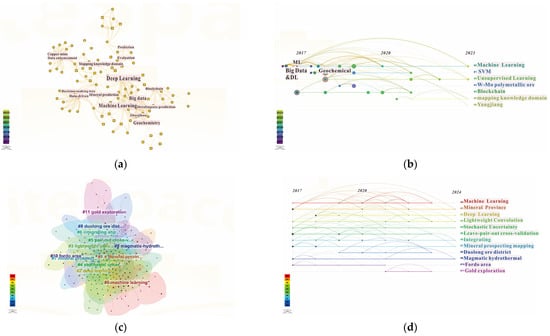
Figure 1.
High-frequency keyword co-occurrence and timeline chart of main keywords in CNKI and WOS (made by Citespace): (a) High-frequency keywords co-occurrence in CNKI; (b) The timeline chart of main keywords in CNKI; (c) High-frequency keywords co-occurrence in WOS; (d) The timeline chart of main keywords in WOS.
3.1. Deep Autoencoder
An autoencoder (AE) is an unsupervised feature learning network that utilizes a backpropagation algorithm so that the target output value equals the input value. The autoencoder consists of an input layer, a hidden layer, and an output layer. After the input layer is input, the data are compressed and encoded in the hidden layer to enhance the characteristics of the data, and then decoded [30,76]; the encoding Formula (1) and decoding Formula (2), respectively, are
where x represents the training data (including bias), We represents the encoder, φ represents the activation function, and Z represents the output value. WD represents the decoder, which translates the output value to the input value. Since the input data and output values of the autoencoder model unit follow the basic logic of a single real neuron [77], the decoding operation process function is an identity function to obtain the output value and the encoded input value.
The Deep Belief Network (DBN) was proposed by Hinton in 2006. It is a probabilistic generation model composed of stacked constrained Boltzmann sets. By training the weights between neurons, the whole neural network can generate training data according to the maximum probability [30,78,79]. The deep autoencoder (DAE) is developed on deep belief networks. First, a model is trained to learn the pattern distribution of the sample, the sample is reconstructed by minimizing the difference between the output value and the input value, and then the sample with a high reconstruction error is identified as an anomaly.
The autoencoder can train samples without difference, reduce the extraction of irrelevant feature information, and it has a good effect on data dimensionality reduction [4,80]. Since the autoencoder has a high reconstruction error for abnormal samples and a low reconstruction error for background samples, it has good applicability in processing geophysical, geochemical, and remote sensing data and can quickly identify data anomalies. According to the metallogenic law and prospecting practice, the formation and discovery of the deposit are small probability events. Anomalies in the data associated with mineralization often belong to low-probability samples, which have little contribution to the autoencoder, so their coding and reconstruction will be poor and have relatively high reconstruction errors [29,30,81]. We can use these data with large reconstruction errors to identify outliers in ore prospecting and prediction.
3.2. Generative Adversarial Network
As a deep generative model, the generative adversarial network (GAN) model is composed of a generative network and a discriminant network. The generative network generates samples close to real samples by learning the distribution of data. The discriminant network is used to evaluate whether the samples are from real samples or generated samples. The two neural network models continue to perform the binary minimax game until the antagonism between the two networks reaches a Nash equilibrium, often used for processing complex, high-dimensional data [82]. Compared with the traditional autoencoder framework, the discriminator added by the generative adversarial network framework has the function of regulating feedback and guiding the generator [29]. For the basic framework of generating adversarial networks, the formula is
Formula (3) is the discriminator loss function, Formula (4) is the generator loss function, x represents the real data, z represents the noise, G stands for generative model, D stands for discriminant model, and G(z) represents the output of an input noise after generating the network; the generator’s goal is to generate data very close to the real data, that is, D(G(z)) as close as possible to 1.
In the process of deep learning, the finiteness and unbalance of geological exploration data often lead to large model errors or strong overfitting characteristics. Using the generative adversarial network to enhance data processing is very suitable to solve the problem of the small number of positive samples of geological data. When processing data with unbalanced positive and negative samples, generative adversarial networks can capture complex patterns and dependencies in the original geological data to generate high-quality sample data [52,83,84]. Farahbakhsh et al. [84] used the generated adversarial network to generate high-quality samples that closely mimic the distribution of underlying data to increase the number of positive samples in the model, effectively solving the problem of unbalanced training data caused by insufficient positive samples in geological data. Wu et al. [52] used conditional generation adversarial networks to add appropriate labels to the initial random noise, generate synthetic samples similar to the original geological data, adjust the distribution of positive and negative samples, and improve the quality of data. The data set model enhanced by the generated adversarial network shows better robustness, the accuracy of the training set and the test set reaches a high level, and the model has better anti-overfitting ability.
The image generated by the generative adversarial network is clearer in the course of training, but it is prone to modal collapse and gradient disappearance [80]. The generative adversarial network also lacks an effective reasoning mechanism, and its data are often difficult to perform an abstract reasoning process with. Some studies have used the correlation between the generative adversarial network and deep autoencoder to train its reasoning ability [85]. Therefore, when predecessors used the generative adversarial network for prospecting prediction, they often used its super ability to generate sample sets for data enhancement operations, and the subsequent prospecting prediction modeling process used other deep learning algorithms. Therefore, when predecessors used the generative adversarial network to make prospecting predictions, they often used its super-strong sample generation ability to enhance the data, and the generated data had better consistency with the original data. On this basis, the researchers combined it with other deep learning methods to make prospecting predictions.
3.3. Convolutional Neural Network
The convolutional neural network (CNN) is a deep feedforward artificial neural network classification method in machine learning, which adopts the idea of the local receptive field, and time or space subsampling, and has the characteristics of translation invariance and shared weight structure, which significantly reduce the number of free parameters in the network. The advantage of the convolutional neural network is that it cannot only learn the overall features of the data, but also learn the local features of the data, and these local features also have a certain correlation. By extracting the features of the deposit data layer by layer, the correlation between mineralization factors and the deposit can be obtained [4,86]. The convolutional neural network is based on images, and the multi-source geological data and remote sensing data used in prospecting prediction can be easily unified into the image format, which provides basic conditions for the convolutional neural website in prospecting prediction [87].
A basic convolutional neural network structure generally includes an input layer, convolutional layer, pooling layer, fully connected layer, and output layer. The input layer takes the original meshed data as the input data. Since the input layer data are not processed, and the hidden layer part cannot be manually intervened, the convolutional neural network avoids the influence that may be brought by the subjective cognition of researchers and their own limitations [34,76,86,88]. Pooling is to compress and converge the data features completed by convolution, reduce the calculation amount, and extract the main features of the data [89]. Two pooling methods are generally selected: average pooling and maximum pooling [86]. Average pooling has relatively low hardware requirements, can reduce the convolutional layer to obtain data redundancy, and retains the diversity of geological features as much as possible. Maximum pooling can highlight the most significant features, reduce the complexity of calculation, and enhance the robustness of the model [9,90]. In the fully connected layer, every node is connected with all the nodes of the previous layer, and the features extracted from the convolutional layer and pooling layer are integrated to achieve feature mapping and classification at the end of the network. The essence of the fully connected layer is a backpropagation neural network [86,88,91].
The general process of the convolutional neural network for prospecting prediction includes the following: data collection and collation—generation of training set, verification set, test set—model construction—training and validation—determination of prospecting prediction region. Since there are many kinds of geological data, convolutional neural networks can fully mine the deep relationships between different kinds of data, which brings great help to the full utilization of data. Therefore, the convolutional neural network is widely used in geological prospecting and prediction.
3.4. Recurrent Neural Network
In the field of deep learning, recurrent neural networks (RNNs) with recurrent connections are capable of processing variable length sequence inputs, modeling sequence data for sequence recognition and prediction, storing information using cyclic iterative functions, and capturing contextual information well. To realize transient dependency learning, the research object is mainly sequence data, such as text, time series data, etc. [92]. The recurrent neural network consists of an input layer, hidden layer, and output layer. In the process of use, people find it difficult to establish long-term dependency, so predecessors have designed more complex activation functions to solve this problem. The most important methods include Long Short-Term Memory (LSTM) (Figure 2) and Gated Recurrent Unit (GRU) [93,94,95]. LSTM is specifically designed for analyzing sequence data, and its main idea is to make predictions through cyclically connected memory units and three key gate units in each memory block (i.e., forgetting gate, input gate, and output gate). Gates are a way to selectively retain or forget information through activation functions [96]. GRUs have gated units that regulate the flow of information within the unit, but do not have separate storage units, showing better performance on smaller data sets [97].
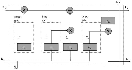
Figure 2.
A basic LSTM block [98]. ft, it, and Ot are outputs of the forget gate, the input gate, and the output gate, respectively, at time step t. Ct − 1 and Ct correspond to the cell state of the time t and time t − 1. t represents the fresh information brought in at time step t. σL and σR are used as the activation function. + represents addition. × represents multiply.
Recurrent neural networks focus on learning the interaction between variables that interact with each other and have the potential to integrate highly correlated geological features for prospecting prediction. LSTM is capable of capturing contextual information within sequences, which complements the limitations of the CNN in context sequence modeling and is the first choice for interpreting geochemical elements related to genesis [99]. This advantage of the recurrent neural network plays a very important role in the use of text-based geological data, which can integrate the original data and extract important information related to mineralization.
4. Application of Deep Learning in Mineral Prospectivity Mapping
4.1. Application of DAE
The deep autoencoder encodes the input data, and the decoder reconstructs the output from the encoding. Because the small probability sample has little contribution to the autoencoder and a high reconstruction error, it has a good advantage in the identification of geochemical anomalies.
Xiong et al. [30] used the deep autoencoder algorithm to identify geochemical anomaly data. Firstly, the deep autoencoder network was constructed, the improved unsupervised building module (Continuous Restricted Boltzmann Machine) was selected as the basis of the deep autoencoder, and the initial weights were pre-trained. Attempts were made to find and enhance correlations between visible and hidden cell values, creating neural networks. The gradient descent technique was used to adjust the network in order to minimize reconstruction errors. Secondly, data preprocessing was carried out, the drainage sediment geochemical data in the study area were selected as the basic data, the closure problem of the basic data was processed by using isometric logarithmic transformation, and the measured values were normalized to the range [0, 1]. Then the model was trained and the parameters were adjusted. Finally, the identification of geochemical data anomalies was carried out. Xiong et al. [30] believe that when applying the deep autoencoder, it is necessary to focus on the setting of learning rate and iteration number, as well as the size of the hidden layer of the geochemical data. When the reconstruction error is minimal and stable, the autoencoder network and its corresponding parameters are optimal for the modeling of geochemical samples. The results show that the geochemical high anomaly area accounts for 2.4% of the total area and 31.5% of the total known iron deposits (Figure 3). The medium anomaly area accounts for 34.1% of the total area and 68.4% of the known iron reserves. Compared with the recognition results of the constrained Boltzmann machine, the results of the deep autoencoder have similar spatial distribution characteristics, which proves that the deep autoencoder has a good ability in geochemical anomaly recognition.
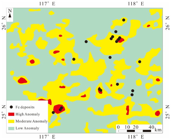
Figure 3.
Spatial relationship between geochemical anomaly maps obtained by DAE and iron ore deposit locations (modified from [30]).
The deep autoencoder plays an important role in identifying anomalies, but the type of anomaly data associated with prospecting prediction requires researchers to analyze the geological evolution process, that is, the judgment of expert experience is needed as the basis for data adoption. When the autoencoder is used for metallogenic prediction, the abnormal regions are often extracted incorrectly due to the high noise of the original data, so some methods need to be used to suppress the noise and reconstruct the error. Research showed that increasing the number of hidden units in the deep autoencoder network can effectively reduce the error between the input data and the generated output value, but this method will greatly increase the risk of overfitting of the model [81], so we need to adjust the parameters repeatedly when using it.
4.2. Application of CNN
The convolutional neural network is the most widely used deep learning algorithm in mineral prospectivity mapping at present, including LeNet, AlexNet, VggNet, GoogleNet, ResNet, U-Net, and other structural types. The main difference between types lies in the structure and depth of the network (Figure 4). The LeNet structure is relatively simple, and people usually choose the Sigmond function or Tanh function as the activation function. Liu et al. [33] applied the convolutional neural network based on LeNet to mine the coupling correlation between the distribution characteristics of elements and the underground placement space of the ore body, and the accuracy rate reached 93%. Xu et al. [100] used the CNN of the LeNet structure to effectively learn the relationship between geological, geophysical, and geochemical data and deposit distribution locations, and the results showed that 90% of known gold deposits were distributed in prospective areas, accounting for only 15% of the studied area. During training, temporarily dropping certain units in the neural network from the network according to a certain probability is Dropout. The AlexNet structure is deeper than the LeNet structure, uses the ReLu function as an activation function to reduce gradient disappearance [101], and performs data enhancement during training, adding Dropout to suppress overfitting. Li et al. [102] used the CNN of the AlexNet structure to learn the internal relationship between geochemical data, sedimentary strata, structure, water system, and other geological information and the location of ore occurrence, and delineated the metallogenic prospect area, and the verification accuracy rate was 86.21%. Li et al. [103] predicted sedimentary manganese ore prospecting in the Songtao–Huayuan area based on the AlexNet network, and obtained a classification model based on the CNN, with an accuracy of 88.89%. VggNet [9,104] has a simple structure and reduces the number of weights by stacking multiple 3 × 3 convolution cores instead of large convolution cores. It also uses ReLU as the activation function after the fully connected layer to suppress overfitting, which is highly applicable. The GoogleNet structure, designed by the Google team in 2014, can extract features from different convolution kernels of feature images in parallel, enriching the information contained in multi-scale feature maps. Multi-source geological data provide the basis for features to integrate feature information with the GoogleNet structure, making this method more suitable for prospecting and prediction [87,105]. ResNet was proposed by He et al. [106] in 2016, aiming to introduce a deep residual learning framework to solve the problem of training accuracy degradation by adding residual structure. ResNet artificially makes certain layers of the neural network skip the connections of the next layer of neurons, connecting the layers separately, weakening the strong connections between each layer. By combining input and output, ResNet effectively alleviates the loss of geo-information caused by convolution operations, and also plays a positive role in solving the problem of gradient disappearance or explosion in deep networks [107,108]. U-Net is a completely updated convolutional neural network with an encoder–decoder structure. The encoder extracts features through convolution, pooling, etc., and gradually reduces the input dimension. According to the data provided by the encoder, the decoder can repair the detailed features to improve the accuracy. Its advantage are that the required training data are smaller, the result is more accurate, and it has an advantage in the processing of small-scale data [109,110,111].
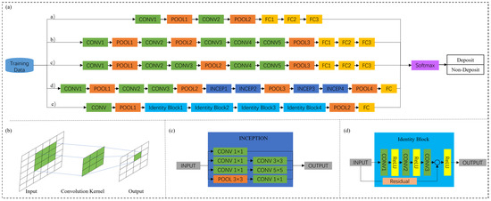
Figure 4.
CCN structures for mineral prospectivity modeling (modified from [9,87,107]): (a) Different CCN structures for mineral prospectivity modeling: a) LeNet, b) AlexNet, c) VggNet, d) GoogleNet; e) ResNet-50; (b) A basic structure for convolution; (c) the detailed process for “Inception” in GoogleNet; (d) the detailed process for “Identity Block” in ResNet-50.
The Nanling area is one of the most important non-ferrous metal metallogenic belts in China, and tungsten tin is the dominant mineral. There are several world-class tungsten tin deposits in this area, such as the Xihuashan tungsten deposit, Dachang Tin deposit, and Shizhuyuan tungsten deposit [112]. Li et al. [36] made use of multivariate data in the area and adopted the convolutional neural network model to make prospecting predictions. The selected data layers included the following: granite and fault; local gravity anomaly closely related to W-Sn ore mineralization; distribution of W, Sn, Bi, Be, Pb, Ag, Mo, and Zn geochemical elements. The buffer zone was delimited according to the distance of the granite and fault, respectively, and the buffer zone map was generated. The geophysical and geochemical data were mapped according to inverse distance weights. Due to insufficient training samples of geological data, the researchers used sliding windows and random zero noise for data enhancement.
Since there are many channels in the geological data layer, the traditional convolutional neural network is complicated to calculate and it is not easy to automatically extract key channel information. A feature of the human visual system is to selectively focus on highlighted parts of the entire scene to better capture the visual structure. Therefore, researchers add an attention mechanism based on the characteristics of the human eye after the convolutional layer to obtain the channel attention graph, which enhances the representation of key features and weakens the performance of channels with low weight values. Its network structure is shown in Figure 5.
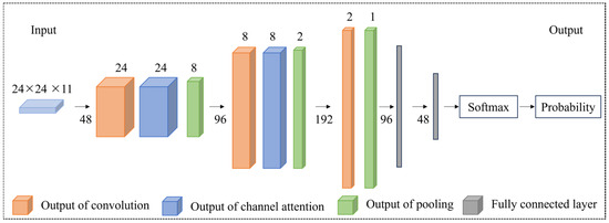
Figure 5.
ATT-CNN structure for mineral prospectivity modeling (modified from [36]).
Combined with the data enhancement method, the researchers built four models separately: a sliding window CNN model, a random zero noise CNN model, an attention-adding mechanism CNN (ATT-CNN) model using a sliding window, and an ATT-CNN model using a random zero noise; a receiver operating characteristic curve (ROC) and an area under ROC curve (AUC) were used to evaluate the accuracy of the prediction model. The experimental results(Figure 6) show that the AUC value of the ATT-CNN model using the sliding window is the highest (0.987), followed by the ATT-CNN model using random zero noise (0.971), the CNN model using the sliding window (0.970), and the CNN model using random zero noise (0.964). This shows that the performance of the convolutional neural network model has been improved after the addition of the attention mechanism, and the recognition ability of important data layers has been enhanced, which provides a good example for prospecting prediction in other areas.
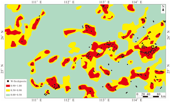
Figure 6.
MPM of W-Sn ore obtained by using sliding window ATT-CNN (modified from [36]).
The following problems should also be paid attention to when using the convolutional neural network for prospecting prediction modeling: the size of the grid, the size of the convolutional kernel, the number of layers, the learning rate, and the number of iterations. The smaller grid can make better use of the existing data and make the calculation more accurate, but it will lead to excessive calculation. If the grid is too large, it cannot effectively use all the data, resulting in reduced accuracy [102]. Zuo [58] studied the size of the output unit and proved that different grid sizes have certain effects on the concentration distribution of geochemical anomalies and the texture structure of different geochemical types. Complex neural networks do not necessarily improve the accuracy of the model. Sun et al. [22] found that in artificial neural networks, the mean squared error of the model does not decrease significantly with the increase in the number of neurons. The learning rate will affect the convergence rate of the model. If the learning rate is too small, the convergence speed will be fast, and if the learning rate is too large, it is difficult to reach the extreme point [9]. In practical application, it is necessary to consider the density and cartographic scale of different types of data samples, and carry out continuous debugging to select the appropriate mesh size, convolutional kernel size, neural network layer number, learning rate, and other parameters.
4.3. Application of RNN
The recurrent neural network has the ability to integrate highly correlated geological features, is very friendly to geological data in geological prospecting and prediction, and has a good application prospect in research areas with abundant geological data. Wang et al. [96] made use of geological, geochemical, and geophysical data in the study area to carry out weight function analysis based on the singularity of deposit location, and built a long and short term memory network model for the evidence layer. The results showed that all known deposits fell in the high prospect area, and 10% of the prospect area accounted for more than 90% of the iron ore deposits. By combining LSTM with the CNN, Wang et al. [99] focused on the inherent feature representation of adjacent samples and the contextual association information learning of geochemical variables, and captured 96% of the granite in 15% of the study area, providing a new idea for the identification of regional geological features and contributing to the mineral prospectivity mapping of areas with insufficient mapping.
The Baguio District of the Philippines is one of the most important gold deposits in the world, with proven gold reserves of more than 800 tons, and the gold deposits are mainly volcanic epithermal deposits. Yin et al. [97] used four types of geological data within the region, such as NE faults, NW faults, Agno magmatite margins, and porphyry intrusive contact zones, as data layers to build models, built buffers and converted grids from the four types of geological data, and used nonlinear control functions of geological characteristics to assign artificial values to grids in all buffers. The data enhancement method was used to generate sufficient samples.
The GRU model in the recurrent neural network was selected to build the model, which includes a cyclic layer, a dense layer, and an activation layer. Its network structure is shown in Figure 7.
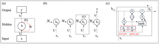
Figure 7.
Data representation for the GRU model (modified from [97]): (a) Basic process of the model; (b) Inner structure of the hidden layer; (c) Inner structure of the GRU. The black arrows represent normal flow and the red arrows represent recurrent connection.
When using recurrent neural network algorithms, the ordering of the evidence layers is critical to the accuracy and predictive power of the final model, and since the GRU can process sequence data through special cyclic states, 24 different input orders can be selected for the four geological evidence layers to model. By analyzing the accuracy, AUC value, Kappa value, Matthews correlation coefficient (MCC), and recall rate of 24 different order models, the researchers determined the optimal evidence layer ranking. The results (Figure 8) show that the sequence beginning with the porphyry intrusion contact zone has better accuracy, while the sequence ending with the porphyry intrusion contact zone has the worst accuracy. In the mineral potential map, the extremely high anomaly area contains 18 deposits, accounting for only 19.23% of the surface, showing good accuracy.
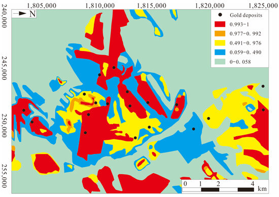
Figure 8.
Mineral potential analysis in Baguio region based on GRU model (modified from [97]).
The experimental results show that the known gold deposits are mainly distributed in the extremely high and high occurrence areas after the classification of the prospect map generated by the GRU by the quantile discontinuous method. The results of the success rate curve evaluation show that the GRU method has better prediction ability.
4.4. Application of GAN
Generative adversarial networks are well suited for enhancing geological data, as they can effectively address the problem of having fewer positive samples. When dealing with imbalanced datasets, generative adversarial networks (GANs) can capture the complex patterns and dependencies present in the original geological data and generate high-quality sample data. GANs can generate fake samples that follow the same population distribution pattern as real samples. GANs have been successfully used in fields such as image processing and earth science.
In the process of actual prospecting work, it is hard to obtain enough positive samples. Jordão et al. [113] proposed a geological model for generating borehole samples, realizing the automatic division of the ore body geological domain based on borehole data by GANs. Li et al. [114] used GANs to enhance geochemical data from rare earth deposits in southwest Jiang, China, and made quantitative measurements of the quality of the augmented data. The test results show that GANs can extract advanced features of real samples and support the synthesis of enhanced data from random inputs.
Guo et al. [115] used a hybrid deep learning method called the SMOTified GAN to detect geochemical anomalies associated with mineralization, which uses SMOTE to generate positive samples, helping to improve the quality of GAN regenerated positive samples. Firstly, a bagging algorithm was used as the integration construction technology and elm as the base classifier as the infrastructure. Secondly, the SMOTified GAN oversampling technique was used to oversample positive samples of geochemical exploration data. Finally, the generated data were used to determine the thresholds for the classification of geochemical anomalies associated with polymetallic mineralization.
The results (Figure 9) show that the high-level anomaly of model recognition is 23.64%. Moreover, the geochemical anomalies associated with polymetallic mineralization in the three identified abnormal areas are highly consistent with the regional geological characteristics and polymetallic metallogenic characteristics of the study area.

Figure 9.
Geochemical anomalies associated with polymetallic mineralization classified by the SMOTified GAN (modified from [115]).
4.5. Application of Mixed Algorithm
Deep learning has a strong ability in data mining, and different deep learning algorithms have slightly different capabilities and focuses in practical applications. With the continuous development of traditional machine learning and deep learning algorithms, the combination of different algorithms has become the main way for researchers to avoid their own defects.
The deep autoencoder can be directly used for prospecting prediction. However, since the noise of its own data is generally large, and the prediction results are easily affected by noise, combining it with the convolutional neural network can help eliminate the influence of noise. Zhang et al. [116] use the Convolutional Autoencoder (CAE) to learn meaningful abstract representations of multi-source geographic information at different scales, and determine the degree of influence of reconstruction errors of each data variable by reducing the removal of evidence variables. The types of geological data that have a greater influence on the reconstruction error are analyzed and the factors that have a greater correlation with mineralization are determined. The core of the CAE is to combine the convolutional operation with the autoencoder structure to form the convolutional encoder and the convolutional decoder, so as to optimize the training results. The success rate curve shows that the predicted potential mineralization area accounts for 23.8% of the study area and contains 77.8% of known gold deposits.
Xie et al. [80] used the combination of the autoencoder and the GAN to conduct metallogenic prediction in the Lhasa area, which not only ensured the stability of the training process, but also ensured the clarity of the training results. The AUC value of the model reached 0.95. The Convolutional neural network mixed the channel information in the process of feature extraction. The combination of the CAE and CNN [29,116] can remove the data types in the evidence layer that have little influence on the reconstruction error, and determine the factors with greater correlation with mineralization. The prediction accuracy AUC value can reach 0.863 and 0.908 in the two regions, respectively.
In order to solve the problem of the lack of labeled data in deep learning algorithms, Li et al. [114] proposed a data enhancement method based on generative adversarial networks, used the enhanced data to carry out research on the convolutional neural network algorithm, and conducted prospecting prediction analysis on rare earth deposits in southern Jiangxi Province, China. The results (Figure 10) show that the GAN can learn the internal structural features of real samples, and can synthesize enhanced data from random inputs. The model training accuracy reaches 99.7%, and the validation accuracy reaches 98.9%. The research also shows that although “black box” is a problem that deep learning cannot avoid, the analysis of prediction results combined with geological and geochemical data can show the reliability and accuracy of deep learning algorithm application.
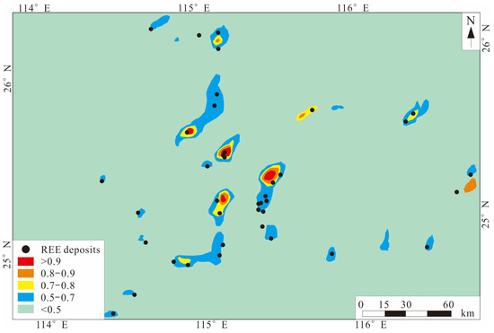
Figure 10.
Regolith-hosted REE deposits prospectivity map derived by the GAN and CNN (modified from [114]).
The combination of different algorithms will provide more ideas and methods for mineral prospectivity mapping.
5. Discussion
5.1. Preprocessing of Geological Data
Geological data are generally text data, geophysical and geochemical data are often point data, and remote sensing data are image data. Different data types need to be preprocessed in different ways when prospecting predictions are made. The uses of various data types are shown in Table 2.
Table 2.
Applications of different data types in MPM.
Geological data generally do not include digital information, and it is difficult for machine learning algorithms to read these text data; geological data use generally two types of methods. One is to select ore-controlling strata and magmatic rocks closely related to mineralization as geological data sources, define different lithologies as different values, and simply classify according to lithology; strata and magmatic rock data mostly adopt this method. Zheng et al. [35] classify different strata according to 1, 2, 3… The unknown geologic body is coded as 0, and the lithology value directly defined during grid training is taken as the grid value. The other type is interpolated according to the distance between strata, structures, and known deposits, the buffer distance is delimited according to the distance size, and the distance value is used directly as the grid value. Researchers often measure the impact of geological formations using the distance from the target location to the structure, converting the data into a distance buffer map that retains distance, position, and orientation information in an image that the machine can recognize. The types of buffer distance graph mainly include the discrete buffer distance graph and continuous buffer distance graph. In the discrete buffer distance graph, the same distance value is in the same “step size” [117,121,122], which simplifies the distance information and makes the calculation more convenient, but this method will reduce the accuracy of the construction information expression. The continuous buffer distance graph uses the continuous value to represent the distance between the target point and the structure, and the result is more accurate and complete [9,22]. Xiong et al. [121], Sun et al. [22], and Yang et al. [9] used the continuous buffer distance to measure the influence range of the geological structure, which better preserved the detailed information of the geological structure in the image, and improved the ability of deposit prediction. In addition, Sun et al. [22] also used the distance between the magma intrusion contact site and the target location and the density of regional faults as the evidence layer of geological characteristics to participate in the modeling. Li et al. [102] used convolutional neural networks to explore the coupling relationship between geological data such as strata, faults, and water systems in the study area and the mining area. In addition, using a natural language model to process earth science text has certain potential in mineral prospect modeling, and has been used in some meaningful applications [123].
It is worth noting that in the process of geological data application, most researchers did not consider the comprehensive use of the relevant characteristics of the whole process of deposit formation, such as source, transport, trap, sedimentation and enrichment, weathering and denudation, etc., and the data types selected were relatively simple, which may have a certain impact on the predicted results. Therefore, it is also necessary to strengthen the exploration of the content, method, and form of geological data types used in deep learning prospecting.
The interpolation of point data sets into raster plots is a common method in geochemical mapping, and the most common method is inverse distance weighted interpolation. The inverse distance weighted interpolation method takes the distance between the interpolation point and the sample point as the weighted average, and the closer to the interpolation point, the higher the weight [27]. The data of geochemical discrete points can be interpolated into the geochemical continuous concentration map, which has a good smoothing effect on the original data. In the past, various univariate or multivariate geochemical statistical analysis methods were used to describe geochemical data and anomalies, requiring normal or lognormal distribution of geochemical data; otherwise, geochemical anomalies could not be correctly identified [81]. In fact, the formation of mineral deposits is a rare event, and the basic requirement of normal or lognormal distribution of geochemical data cannot be guaranteed. Traditional multivariate statistical methods often lose their function when dealing with geochemical data under complex conditions, but deep learning algorithms can learn the deep-level evidence information in the data without data processing. Sometimes geochemical data are the composition of a certain substance, for example, H is a part of H2O, the content of H is correlated with H2O, and the contribution of H to statistical analysis is very likely to represent the contribution of H2O to statistical analysis, which will lead to closure problems in multivariate statistical analysis [124]. The researchers used the method of isometric logarithmic ratio transformation to process the raw data.
In addition, geochemical data of rocks or mineral deposits, such as major trace elements, hydrogen and oxygen isotopes, Re-Os isotopes, U-Th-Pb isotopes, Sr-Nd isotopes, etc., are not stable and representative of in situ data due to their sampling locations and sampling principles different from grid sampling of ordinary geophysical and geochemical data. Therefore, this type of data is generally not used. However, when part of the data has in situ data characteristics and has a certain correlation with mineralization, it can be selected as a feature of deep learning to participate in the calculation.
The geochemical data often come from or are close to the earth’s surface and may not necessarily include key ore-controlling geological factors, which can lead to a poor MPM result [125]. Li et al. [102] made use of the method of coupling geochemical data with geological data, projected the information of geological data onto geochemical data, and used deep learning to make better use of geochemical data for prospecting and prediction, achieving good results and providing us with new ideas for using geological data.
Remote sensing data itself has the characteristics of multi-dimensional numbers, uneven noise, and so on, which brings many problems to data processing. However, deep learning can extract useful features from massive remote sensing data, and has great potential in mineral deposit classification and prospecting prospect prediction. The recognition of remote sensing images related to mineralization mainly includes the recognition of a linear ring structure and the recognition of surrounding rock alteration. Zidan et al. [68] used the deep learning algorithm of the CNN to extract hydrothermal alteration regions related to porphyry copper deposits based on ASTER images, and delineated the scope for further determining the potential areas for prospecting. Sun et al. [22] used the iron oxide alteration and mud alteration obtained from Landsat ETM+ images as evidence layers and other geological data to conduct deep learning modeling and delineate the prospecting target area, providing an important basis for further prospecting and exploration. Fu et al. [27] used the CNN algorithm based on GF-5 remote sensing images, ASTER images, and geochemical data to predict the mineral prospect area in the Duolong region of Tibet, and used alteration minerals such as dolomite and kaolin, identified by the short-wave infrared band, as the evidence layer to construct the CNN model for prospecting prediction. The results show that the alteration zone extracted from remote sensing images has good indication significance for prospecting prediction. Therefore, the processing of remote sensing data mainly uses a variety of image processing techniques to extract geological structure information and alteration information as data layers for deep learning modeling.
By summarizing the previous studies, we find that geochemical data, geological data, and remote sensing data are widely used in prospecting prediction, the research methods are increasing, and the varieties are becoming more and more abundant. As an important means of prospecting and exploration, geophysical methods have more and more diversified physical property types and data forms. As geophysical methods play an increasingly important role in deep prospecting, geophysical data as the evidence layer of deep learning algorithms can help improve the accuracy and generalization ability of the model. Sun et al. [22] used gravity data, aeromagnetic exploration data, and resistivity data in the Tongling area of Anhui Province, China to generate a magnetic anomaly pole map, lithology density map, −800m resistivity interpretation map, and other geological data as data layers. Based on the source, transport, and storage processes of mineralization, the support vector machine, random forest, and machine learning algorithms were used to model and analyze the ore prospecting prediction, the ore prospecting prediction in the study area was evaluated, and the favorable metallogenic prediction area was delineated. Wang et al. [96] used aeromagnetic data combined with regional granite mass, regional major faults, and geochemical data to predict the iron ore prospecting potential in Fujian Province, China, and the results showed the feasibility and reliability of prospecting prediction by using aeromagnetic data. However, due to the multi-solution of geophysical data, there are still some limitations in geological prospecting prediction, and the application of geophysical data in deep learning prospecting is not extensive enough. The next step is to combine geophysical data with geological data to improve the coupling ability of geophysical data and ore deposits.
5.2. Improvement of Data Enhancement Method in Mineral Prospectivity Mapping
Machine learning for prospecting prediction is essentially a binary classification problem, and the result is to classify each area as promising or unpromising [18,22]. In areas with few ore deposits or where no ore deposits have been found, there are not enough data samples to reach the amount of data required by deep learning, and there is poor extraction of ore-related features, poor generalization ability of the resulting model, and even non-convergence of prediction results. Therefore, sufficient training samples are the key to the success of the model. In order to ensure the robustness of the model, the positive and negative samples in the sample set need to be relatively balanced. However, in reality and prospecting practice, the samples with ore deposits are much larger than the samples without ore deposits, resulting in the imbalance between positive and negative samples. Due to the small number of geological data samples, it is an urgent problem to enhance them in machine learning algorithms.
Data enhancement is the use of a series of methods to expand the amount of data to overcome the lack of deep learning training samples. The traditional data enhancement methods generally use inversion, distortion, rotation, clipping, and other deformation operations to increase the number of samples, but in geological prospecting work, these methods cannot increase the effective training samples, and may even make the final result progress in the opposite direction. Therefore, researchers continue to develop more feasible data enhancement methods in geological work, mainly including the sliding window, clipping and patching, adding random noise, etc., and with the development of deep learning, the CAE and GAN can also play an important role in data enhancement due to their excellent data generation capabilities. Table 3 lists the application of different data enhancement methods in prospecting prediction.
Table 3.
Application of different data enhancement methods.
Sliding window is a commonly used data enhancement method. Core areas are selected at each evidence layer in turn, a window smaller than the core area is used to slide in the area for resampling, and then resampling results of each evidence layer are combined. The generated window remains in the core area until the required number of samples is generated. The advantage of sliding windows is that new data can carry all the information in the original evidence layers and resampling. Wu et al. [52] use sliding window technology to enhance data samples and solve the problem of scarcity and imbalance of label data in deep learning environments.
Adding random zero noise is another processing method. By adding zero noise points to the original evidence layer and combining the original evidence layer to achieve the purpose of increasing data, this method can maintain the original geographical location, correlation, and other relative information of the data, and can maintain the integrity of the data and highlight the overall characteristics of the data. However, it is necessary to consider the ratio of random zero noise when using it. Adding different ratios of zero noise will make the generated sample data carry different characteristics. The purpose of adding zero noise is to generate more samples to expand the data, and from the experience of previous people, the random noise ratio is set between 5% and 10% for the best effect.
In addition, Brandmeier et al. [127] increased the number of training samples by disturbing the location of the deposit and adding data points around the real deposit. Yang et al. [9,87] used a clipping and repairing method to generate additional training samples. This method not only ensured that the expanded sample data and the test data had similar deposit indication characteristics and deposit location, but also ensured that the expanded sample data and the test data had different combinations of multi-source geographic information in different spatial locations, which has a good reference significance. Zhang et al. [126] used the pixel-to-feature method to reassemble the pixels of the sample to generate enough training samples.
With the development of deep learning algorithms, researchers use the GAN and other algorithms based on sample data to generate more usable sample sets, which can retain deeper features in the original samples. Wu et al. [52] add random noise to the original data, combine corresponding label information from real samples to generate basic data, and use the generated adversarial network for data enhancement, which is essentially a comprehensive application of adding random noise and the GAN. Li et al. [114] also used the GAN to enhance the geochemical data, which achieved good results.
5.3. Deep Learning in Mineral Prospectivity Mapping
Compared with traditional statistical analysis methods such as the evidence weight method, information content method, regression analysis, support vector machine, random forest, and other traditional machine learning algorithms, deep learning can directly extract key features from the original data without the need for manual design or selection in advance. By building multi-level neural networks, deep learning is able to capture nonlinear relationships in data, so it has strong data fitting ability, which makes deep learning achieve better results when solving complex problems. When the geological data are comprehensively utilized, the number of channels is large, and the deep learning algorithm can fully meet the practical application of prospecting prediction. Fu et al. [27] used remote sensing images and geochemical data to make prospecting predictions of the Duolong porphyry copper mine in Xizang, China. The AUC value of the CNN model was 0.982, which was better than that of random forest and the support vector machine (0.973 and 0.959, respectively). Wang et al. [96] conducted prospecting prediction in iron ore deposits in Fujian, China. According to the success rate curve, the recurrent neural network and logistic regression model accounted for more than 90% and 80% of iron ore deposits, respectively, in 10% prospective areas, and the linear regression results were significantly better. According to previous studies, deep learning algorithms have been applied to various types of minerals such as Au, Fe, Cu, W-Sn, Pb-Zn, REE, etc., with good effect, and their future application prospects are very wide.
In the field of mineral prospectivity mapping, the application of deep learning algorithms is gradually increasing, which significantly improves the efficiency and accuracy of mineral resource exploration. Different algorithms are suitable for different application scenarios because of their unique advantages. For example, GANs are mainly used in data enhancement, DAEs are used in data enhancement and denoising, RNNs are widely used in text information extraction and time series data analysis, and CNNs are widely used in geological image analysis and processing to identify mineralization features and geological structures due to their excellent performance in image processing, providing an important basis for prospecting prediction. Table 4 lists the application examples of deep learning algorithms in prospecting prediction. In terms of data volume, compared with traditional statistical analysis methods, deep learning has a very strong data processing ability, and geological data processing of mineral deposits, mining areas, and regions can be completed. The number of iterations, learning rate, and batch size of deep learning are greatly affected by the quality of the original data. Due to the imbalance of positive and negative samples, data noise, and other problems in the original data, it is often necessary to conduct several iterations to stabilize the model. From the perspective of model accuracy of deep learning, the AUC value is generally greater than 0.8, and in convolutional neural networks, the AUC value can even reach more than 0.98, which is far more accurate than traditional algorithms. It can be seen that deep learning algorithms have the ability to mine deep features in complex data and hidden associations between data.
Table 4.
The practical application of different algorithms in mineral prospectivity mapping.
However, we should also note that deep learning algorithms have certain limitations, specifically including the following questions:
- (1)
- The support for the algorithm by textual geological data. Deep learning algorithms need to convert some text information into numerical information for computation. In the application of geological information, the data can only be displayed, but a lot of geological information will be discarded. For example, when applying fault data, the distance between different positions and faults will be reflected, but different types of faults will not be reflected, which is unreasonable in geological understanding. Natural language processing (NLP) is a branch of computer science and artificial intelligence that studies how computers understand, generate, and translate human language. RNNs can process sequence data and are particularly effective for natural language processing tasks, so the application of RNNs in geological data can be increased in future research.
- (2)
- The research on geological data enhancement methods. Data enhancement can enrich data, but the large-scale use of data enhancement methods will increase the complexity of training, sometimes resulting in some categories being “over-enhanced”, and others being ignored, resulting in an imbalance between categories. Nowadays, many scholars try to use the combination of transfer learning and deep learning for rock and ore analysis and mineral prospecting prediction [108,129,130,131]. The robustness and generalization ability of transfer learning are proved, the convergence speed of deep learning is accelerated, and the learning efficiency of the prospecting prediction model is enhanced. So, we believe that the use of transfer learning and the adversarial generation network in the future will greatly improve the reliability and logic of enhanced data, which will greatly improve the accuracy of prospecting prediction.
- (3)
- Avoidance and treatment of model overfitting. Overfitting often occurs when testing with a small number of training sets, and will greatly affect the test results and the performance of the model. The most direct way to improve the performance of neural networks is to increase the number of parameters such as depth and network, but this will make it easier for the updated network to reach the overfitting state, especially when the number of positive samples, such as in prospecting prediction, is limited. At present, in other fields, the methods to solve the overfitting of deep learning models mainly include data preprocessing, simplifying the model structure, adding regularization terms, adding Dropout layers, and adjusting model parameters. In mineral prospectivity mapping, the application of Dropout layers has achieved good results. Krizhevsky et al. [101] solve the overfitting problem by increasing the number and size of layers while using the method of Dropout. Li et al. [117] believe that increasing the number of layers and parameters will increase the computational amount of learning, and adding Dropout can reduce the training time during the training process with a large amount of data. Moreover, from the application point of view [90], after using Dropout, the hidden neurons no longer depend on the existence of other hidden neurons, and the co-adaptability with other neurons decreases, which has a good effect on solving the overfitting problem. In the next research process, the diversity of data can be increased in the data preprocessing process, and the learning rate, batch size, and other parameters in the model can be adjusted in time.
- (4)
- Adjustment of parameters of the model. In some research examples, we can see that researchers often need to constantly try to modify various parameters, such as the learning rate, the epoch, the batch size, and so on, according to the size of data or the quality of data to obtain better prediction results. This is because the deep learning model needs to optimize the performance of the model by adjusting parameters during the training process, so that it can better fit the training data and generalize to the unseen data. Therefore, we may need to continue to strengthen the self-adaptive research of the model, so that the model can automatically adjust parameters according to the original data and the target.
- (5)
- The choice of backbone architecture and the effectiveness of different deep learning algorithms. Convolutional neural network is the most widely used deep learning algorithm in mineral prospectivity mapping at present, including LeNet, AlexNet, VggNet, GoogleNet, ResNet, U-Net and other structural types. The most common methods of recurrent neural networks include Long Short-Term Memory (LSTM) and Gated Recurrent Unit (GRU). We need to choose the backbone architecture and deep learning algorithms according to the actual situation.
- (6)
- The explanation of the model “black box” mechanism. The “black box” mechanism of deep learning cannot know about the drivers of underlying phenomena and processes [125], so the interpretability of model outputs, the relationship between data input and output, and the internal operation mechanism need further study. At present, the Google DeepMind team is exploring the “black box” mechanism in deep learning from the perspective of cognitive psychology [132], but there is still a long way to go. To enhance the explainability of deep learning, Fu et al. [27] used the SHAP library in Python to explain the individual output results of deep learning. The results showed that the different types of data selected for distinguishing between the presence and absence of minerals in the study area are of significantly different importance. Many scholars have found that the predictive results of deep learning are not as good as those of SVM or random forest algorithms in some cases, and a major reason for this is the type of data used [4,22].
5.4. Accuracy Evaluation Method in Mineral Prospectivity Mapping
Accuracy is the proportion of samples with correct prediction in all samples [36], and accuracy can directly reflect the proportion of correct classification; the calculation of accuracy is very simple. However, in the process of mineral prospectivity mapping, the number of samples with ore is often small, and the accuracy rate will lose its significance due to the extreme imbalance of positive and negative data. Therefore, other evaluation methods are often used in the prediction and evaluation of prospecting.
The recall rate represents the proportion of positive samples predicted correctly in all positive samples, and precision represents the proportion of positive samples with correct prediction and all samples with correct prediction. Generally, the recall rate and precision are combined, and the harmonic mean of the recall rate and precision (F1 value) is used for comprehensive evaluation. The recall rate and precision index are suitable for the binary classification index, and it is a binary classification calculation model that we need to determine whether there is an ore deposit in prospecting prediction, so the recall rate and precision index are suitable for prospecting prediction and evaluation.
R represents the recall rate, P represents the precision, TP represents the number of actual true predictions that are true, FN represents the number of actual true predictions that are false, FP represents the number of actual false predictions that are true, and F1 represents the harmonic mean of the recall rate and precision.
Accuracy function and loss function can also be used to evaluate the accuracy of deep learning. A better effect needs a smaller loss function and a higher accuracy [35]. Generally, the receiver operating characteristic curve (ROC) and Area Under the Curve (AUC) are used for accuracy evaluation.
TPR represents the true rate, FPR represents the false positive rate, and TN represents the number of predictions that are false and actually false. It can be seen from the formula that TPR is the same as the recall rate.
The vertical coordinate of the ROC curve is the true rate, and the horizontal coordinate is the false positive rate. The TPR is the probability of being judged to be true in the true sample, and the FPR is the probability of being misjudged to be true in the false sample. The advantage of the ROC curve is that in the evaluation process, it is not necessary to add a number as the judgment value of the evaluation, and the accuracy level of the prediction results can be analyzed only according to the below-line area.
The Kappa coefficient is the proportion of correct classification after the removal of accidental coincidence probability, and the calculation formula of the Kappa coefficient is
Po is the accuracy of prediction, that is, the consistency of model prediction results and actual classification results. Pe is accidental consistency, that is, the consistency between two variables (in this case, the classification result and the validation sample); even if the two variables are completely independent, it will not be 0, and there are still cases where chance causes the two variables to be consistent. Using the Kappa coefficient to evaluate the reliability of prospecting prediction models can often increase the difference between different models and make the advantages of models more prominent.
The predicted area curve composed of the prediction rate and area rate is another method of accuracy evaluation. The intersection point of the two curves of deposit proportion and occupied area proportion is taken as the evaluation standard. When the intersection point of the two curves is closer to the top position, it means that more deposits are contained in fewer areas, indicating that the prediction effect is more ideal [4,87,133,134].
In mineral prediction, researchers often use the success rate curve to evaluate the accuracy of the prospecting prediction model with the success rate of known deposit prediction, in which different slopes represent different ore-forming potentials, and the steeper the slope, the more deposits are captured in smaller areas [4,135]. The higher the success rate and the more deposits captured in a smaller area, the higher the accuracy of the model and the better the prediction effect.
The accuracy rate is the proportion of correctly classified samples in the total samples, it is easy to understand and explain, and in the case of a relatively balanced number of positive and negative samples, accuracy can better reflect the overall performance of the model. However, when the number of positive and negative samples is unbalanced, the accuracy will be biased towards the majority class, which may lead to insufficient recognition ability for the minority class. The accuracy rate cannot reflect the ability of the model to recognize positive and negative samples alone, so it is necessary to evaluate the performance of the model in combination with other indicators. The recall rate measures how many truly positive samples the model is able to identify and is very sensitive to unbalanced data sets. However, the recall rate may ignore the ability to identify negative samples, and in the binary classification problem, different thresholds will lead to different recall rates, so it is necessary to choose the appropriate threshold according to the specific situation. The PR curve (precision rate–recall curve) is used to evaluate the performance of the model in a specific category, especially a few categories [96]. It has recall as the horizontal axis and precision as the vertical axis. The recall rate represents the proportion of all positive samples that are correctly judged to be positive; the accuracy rate represents the percentage of all samples judged to be positive that are actually positive. The PR curve has higher sensitivity when dealing with unbalanced data sets, so it has a good application prospect for accuracy evaluation in mineral prospectivity mapping. The ROC curve is mainly used to evaluate the performance of classification models, especially in binary classification problems, which can provide for the performance of models under different thresholds. The Kappa coefficient is mainly used to evaluate the model accuracy of multiple classification problems, especially when the consistency between evaluators is more common. Success rate curves can be used to show how the model performs at different thresholds, providing more detail. Nowadays, ROC and AUC, the predicted area curve, and success rate curve are widely used, respectively, in prospecting prediction activities (Table 5).
Table 5.
Application of different accuracy evaluation methods in MPM.
At the same time, the confusion matrix, mean squared error series, and Brier score are often applied to deep learning tasks. The confusion matrix is a specific table used to visualize the performance of an algorithm, showing how the actual class compares to the predicted class. The overall performance of the model can be assessed by size; the larger the value on the diagonal, the better. But the confusion matrix may not work well for extremely unbalanced data sets, as the performance of a few classes may be overshadowed by the performance of the many classes. Therefore, it is necessary to use this method carefully when making prospecting predictions. Mean squared error (MSE), Root mean squared error (RMSE), and Mean absolute error (MAE) are used to measure the difference between the predicted value and the actual value. The smaller the MSE and RMSE, the more accurate the model prediction, while MAE directly reflects the average level of prediction error. MSE is very sensitive to large deviations between predicted and actual values. Since the errors are squared, larger errors will be penalized more severely, which helps the model better capture and reduce these large errors. MSE, RMSE, and MAE are very sensitive to small probability metallogenic events, but they are widely used in regression problems, reflecting the overall error level of numerical prediction, so these evaluation methods can be used carefully in future studies about mineral prospectivity mapping. The Brier score is the mean square error of the difference between the forecast probability and the actual result, and is often used to evaluate the degree of calibration and accuracy of probabilistic models; the closer to 0 the prediction is, the better the prediction is. The Brier score is sensitive to the change in predicted value near 0 or 1, which has a good application space in deep learning prospecting prediction. Prediction accuracy evaluation methods are varied. In practical application, in order to avoid various curves that may exist in a single accuracy evaluation method, several different accuracy evaluation methods can be used to comprehensively judge the reliability of the model. In the future, we also need to continue to try to apply various other accuracy assessment methods to deep learning in mineral prospectivity mapping.
In addition, we need to consider the influencing factors of accuracy evaluation. By summarizing the previous research process, we believe that the accuracy of the results is mainly affected by the following reasons:
- (1)
- Type and accuracy of data. The correlation between the data and the ore deposit and the number of data types affects the prediction accuracy. Yang et al. [9] selected three kinds of geological data and eight kinds of geochemical prospecting factors, for a total of 11 predictive variables, to predict gold deposits in Fengxian County in China by the CNN, and the training accuracy was 1.00. Liu et al. [33] only selected Pb in the geochemical element to predict lead–zinc ore deposits in Anhui, China, and a training accuracy of 0.93 was obtained. The accuracy of the data affects the prediction accuracy all the same. Li et al. [117] selected 1:200,000 geochemical data to use for mineral prospectivity mapping in the southwestern Fujian Province, China, and the accuracy was 0.95. Using 1:50,000 stream sediment geochemical survey data, Fu et al. [27] predicted the deposit with an accuracy of 0.993. The study of Zuo [58] shows that the size of different scales has a slight influence on metallogenic prediction.
- (2)
- The number and distribution of known deposits. It is clear that the number of known mineral sites in the study area determines the prediction results. More importantly, due to the spatial heterogeneity of the deposit itself, the spatial distribution characteristics of known deposits also affect the prediction results. Therefore, collecting more comprehensive ore deposits in the study area will be helpful for prospecting prediction.
- (3)
- Types of algorithms. The metallogenic systems and processes under different regional frameworks are discrepant, so we should select the data type according to the characteristics of the study area to be used for metallogenic prediction, then select targeted deep learning algorithms according to different data characteristics. Luo et al. [120] efficiently extracted anomalies from geochemical data using the GAN, and the corresponding AUC was 0.893. Wang et al. [96] used a Long Short-Term Memory network to extract and integrate the deep-level geological prospecting information among the weighted evidence layers, and almost all known iron ore deposits developed in delineated high prospective areas. We believe that the selection of deep learning algorithms should rely on the comprehensive consideration of data types and regional characteristics.
Therefore, when applying deep learning to mineral prospecting mapping, we should first collect data comprehensively and accurately to ensure that the type of data is comprehensive and the accuracy is reliable, and then carefully consider the selection of data and the application of methods according to the distribution characteristics of known deposits.
6. Conclusions
As a new data-driven model, deep learning algorithms can directly extract key features from the original data by building multi-layer neural networks, which can capture nonlinear relationships and demonstrate powerful data fitting capabilities. At present, they are widely used in geological prospecting and prediction, and applied to a certain extent in various ore deposits, with good results and optimistic prospects for future application. Compared with traditional prospecting prediction, deep learning algorithms have obvious advantages, and different types of deep learning algorithms, including the DAE, CNN, RNN, GAN, etc., have enhanced the development of prospecting prediction methods to varying degrees, and are of great significance to mineral development. Integrated methods currently used in exploration projects, such as integrated geophysical inversion methods and joint optimization methods, can also be integrated with deep learning in mineral prospectivity mapping in the future.
Multivariate geological data, data enhancement, and deep learning algorithms are three important components of deep learning-based mineral prospectivity mapping. However, at present, there are some challenges in mineral prospectivity mapping using deep learning, mainly including the poor quality of geological basic data, the applicability of data enhancement methods, the interpretability of deep learning algorithms, and the selection of prediction accuracy evaluation methods.
The application of deep learning in prospecting prediction is very effective, the prospect is objective, and it can provide new ideas for future prospecting. The main research directions of future deep learning in mineral prospectivity mapping are the category extension and processing method of geological data, the further study of data enhancement methods, and the comprehensive application of deep learning algorithms to give full play to their respective advantages. Solving these problems will help deep learning make greater progress in the field of mineral prospectivity mapping.
Author Contributions
Conceptualization, Y.C., G.G. and K.S.; formal analysis, K.S., Y.Z. and Z.L.; writing—original draft preparation, K.S.; writing—review and editing, K.S., Y.C. and W.Z.; supervision, J.G., Z.S., Z.L. and Z.Z. All authors have read and agreed to the published version of the manuscript.
Funding
This research was funded by the Program of China Geological Survey (project numbers DD20243184, DD20230591, DD20243187).
Conflicts of Interest
The authors declare no conflicts of interest.
References
- Zhang, S. Multi-Geoinformation Integration for Mineral Prospectivity Mapping in the Hezuo-Meiwu District, Gansu Province. Ph.D. Thesis, China University of Geoscience, Beijing, China, 2022. [Google Scholar]
- Zhao, P. Quantitative mineral prediction and deep mineral. Earth Sci. Front. 2007, 14, 001–010. [Google Scholar]
- Xiao, K.; Ding, J.; Liu, R. The Discussion of Three-part Form of Non-fuel Mineral Resource Assessment. Geol. Rev. 2006, 52, 793–798. [Google Scholar] [CrossRef]
- Yang, N.; Zhang, Z.; Yang, J.; Hong, Z. Mineral Prospectivity Prediction by Integration of Convolutional Autoencoder Network and Random Forest. Nat. Resour. Res. 2022, 31, 1103–1119. [Google Scholar] [CrossRef]
- Carranza, E.J.M.; Laborte, A.G. Data-driven predictive mapping of gold prospectivity, Baguio district, Philippines: Application of Random Forests algorithm. Ore Geol. Rev. 2015, 71, 777–787. [Google Scholar] [CrossRef]
- Carranza, E.J.M. Geocomputation of mineral exploration targets. Comput. Geosci. 2011, 37, 1907–1916. [Google Scholar] [CrossRef]
- Porwal, A.; Carranza, E.J.M. Introduction to the Special Issue: GIS-based mineral potential modelling and geological data analyses for mineral exploration. Ore Geol. Rev. 2015, 71, 477–483. [Google Scholar] [CrossRef]
- Zhang, D. Spatially Weighted Technology for Logistic Regression and Its Application in Mineral Prospective Mapping. Ph.D. Thesis, China University of Geoscience, Wuhan, China, 2015. [Google Scholar]
- Yang, N.; Zhang, Z.; Yang, J.; Hong, Z. Applications of data augmentation in mineral prospectivity prediction based on convolutional neural networks. Comput. Geosci. 2022, 161, 105075. [Google Scholar] [CrossRef]
- Singer, D.A. Basic concepts in three-part quantitative assessments of undiscovered mineral resources. Nonrenew. Resour. 1993, 2, 69–81. [Google Scholar] [CrossRef]
- Zhao, P.; Hu, J.; Li, Z. The theory and practices of statistical prediction for mineral deposits. Earth Sci.- J. Wuhan Coll. Geol. 1983, 4, 107–121. [Google Scholar]
- Cheng, Q. Ideas and methods for mineral resources integrated prediction in covered areas. Earth Sci.- J. Wuhan Coll. Geol. 2012, 37, 1109–1125. [Google Scholar]
- Agterberg, F.P.; Cheng, Q. Conditional Independence Test for Weights-of-Evidence Modeling. Nat. Resour. Res. 2002, 11, 249–255. [Google Scholar] [CrossRef]
- Cheng, Q. BoostWofE: A New Sequential Weights of Evidence Model Reducing the Effect of Conditional Dependency. Math. Geosci. 2015, 47, 591–621. [Google Scholar] [CrossRef]
- Chen, S. Research of Multiple Geoscience Information Prospecting Prediction in Xikuangshan Antimony Ore Field. Ph.D. Thesis, China University of Geoscience, Beijing, China, 2012. [Google Scholar]
- Li, X.; Yuan, F.; Zhang, M.; Jia, C.; Jowitt, S.; Ord, A.; Zheng, T.; Hu, X.; Li, Y. Three-dimensional mineral prospectivity modeling for targeting of concealed mineralization within the Zhonggu iron orefield, Ningwu Basin, China. Ore Geol. Rev. 2015, 71, 633–654. [Google Scholar] [CrossRef]
- Porwal, A.; González-Álvarez, I.; Markwitz, V.; McCuaig, T.C.; Mamuse, A. Weights-of-evidence and logistic regression modeling of magmatic nickel sulfide prospectivity in the Yilgarn Craton, Western Australia. Ore Geol. Rev. 2010, 38, 184–196. [Google Scholar] [CrossRef]
- Zuo, R.; Carranza, E.J.M. Support vector machine: A tool for mapping mineral prospectivity. Comput. Geosci. 2011, 37, 1967–1975. [Google Scholar] [CrossRef]
- Shabankareh, M.; Hezarkhani, A. Application of support vector machines for copper potential mapping in Kerman region, Iran. J. Afr. Earth Sci. 2017, 128, 116–126. [Google Scholar] [CrossRef]
- Chen, Y.; Wu, W. Application of one-class support vector machine to quickly identify multivariate anomalies from geochemical exploration data. Geochem. Explor. Environ. Anal. 2017, 17, 231–238. [Google Scholar] [CrossRef]
- Chen, Y.; Wu, W. Mapping mineral prospectivity by using one-class support vector machine to identify multivariate geological anomalies from digital geological survey data. Aust. J. Earth Sci. 2017, 64, 639–651. [Google Scholar] [CrossRef]
- Sun, T.; Chen, F.; Zhong, L.; Liu, W.; Wang, Y. GIS-based mineral prospectivity mapping using machine learning methods: A case study from Tongling ore district, eastern China. Ore Geol. Rev. 2019, 109, 26–49. [Google Scholar] [CrossRef]
- Carranza, E.J.M.; Laborte, A.G. Random forest predictive modeling of mineral prospectivity with small number of prospects and data with missing values in Abra (Philippines). Comput. Geosci. 2015, 74, 60–70. [Google Scholar] [CrossRef]
- Wang, Z.; Zuo, R.; Dong, Y. Mapping geochemical anomalies through integrating random forest and metric learning methods. Nat. Resour. Res. 2019, 28, 1285–1298. [Google Scholar] [CrossRef]
- Gao, Y.; Zhang, Z.; Xiong, Y.; Zuo, R. Mapping mineral prospectivity for Cu polymetallic mineralization in southwest Fujian Province, China. Ore Geol. Rev. 2016, 75, 16–28. [Google Scholar] [CrossRef]
- Zhang, F.M.A. Research on Deep Learning Extraction Method in Open Mining Area Based on Multi-Source Remote Sensing Images; Anhui University: Hefei, China, 2020. [Google Scholar]
- Fu, Y.; Cheng, Q.; Jing, L.; Ye, B.; Fu, H. Mineral Prospectivity Mapping of Porphyry Copper Deposits Based on Remote Sensing Imagery and Geochemical Data in the Duolong Ore District, Tibet. Remote Sens. 2023, 15, 439. [Google Scholar] [CrossRef]
- Feng, J.; Zhang, Q.; Luo, J. Deeply mining the intrinsic value of geodata to improve the accuracy of predicting by quantitatively optimizing method for prospecting target areas. Earth Sci. Front. 2022, 29, 403–411. [Google Scholar] [CrossRef]
- Zhang, C.; Zuo, R. Recognition of multivariate geochemical anomalies associated with mineralization using an improved generative adversarial network. Ore Geol. Rev. 2021, 136, 104264. [Google Scholar] [CrossRef]
- Xiong, Y.; Zuo, R. Recognition of geochemical anomalies using a deep autoencoder network. Comput. Geosci. 2016, 86, 75–82. [Google Scholar] [CrossRef]
- Zuo, R.; Xiong, Y. Big Data Analytics of Identifying Geochemical Anomalies Supported by Machine Learning Methods. Nat. Resour. Res. 2018, 27, 5–13. [Google Scholar] [CrossRef]
- Shi, L.; Jianping, C.; Jie, X. Prospecting Information Extraction by Text Mining Based on Convolutional Neural Networks–A Case Study of the Lala Copper Deposit, China. IEEE Access 2018, 6, 52286–52297. [Google Scholar] [CrossRef]
- Liu, Y.; Zhu, L.; Zhou, Y. Application of Convolutional Neural Network in prospecting prediction of ore deposits: Taking the Zhaojikou Pb-Zn ore deposit in Anhui Province as a case. Acta Petrol. Sin. 2018, 34, 3217–3224. [Google Scholar]
- Liu, Y. Experimental research on big data mining and intelligent prediction of prospecting target area—Application of convolutional neural network model. Geotecton. Metallog. 2020, 44, 192–202. [Google Scholar]
- Zheng, X.; Zhang, M.; Ren, W. Application of convolution neural networks in gold exploration and prediction in Shandong Province. Geophys. Geochem. Explor. 2023, 47, 1433–1440. [Google Scholar]
- Li, Q.; Chen, G.; Luo, L. Mineral prospectivity mapping using attention-based convolutional neural network. Ore Geol. Rev. 2023, 156, 105381. [Google Scholar] [CrossRef]
- Li, Y.-S.; Chai, S.-L. Soil geochemical prospecting prediction method based on deep convolutional neural networks-Taking Daqiao Gold Deposit in Gansu Province, China as an example. China Geol. 2022, 5, 71–83. [Google Scholar]
- Du, Y.; Cao, Y.; Huo, D.; Li, D.; Gao, Z. Petrology and geochemistry of Silurian-Triassic sedimentary rocks in the Tongling area; Constraints on the genesis of stratabound skarn deposits. Earth Sci. Front. 2014, 21, 228–239. [Google Scholar]
- Ling, Q.; LIU, C. REE behavior during formation of st ra ta-bound skarn and related deposit: A case study of Dongguashan ska rn deposit in Anh ui province, China. Acta Petrol. Sin. 2003, 19, 192–200. [Google Scholar]
- Deng, Y.; Song, X.; Jie, W.; Yuan, F.; Zhao, Z.; Wei, S.; Zhu, J.; Kang, J.; Wang, K.; Liang, Q.; et al. Determination of sedimentary ages of strata in the Huangshan-Jingerquan mineralization belt and its geological significance. Acta Geol. Sin. 2021, 95, 362–376. [Google Scholar] [CrossRef]
- Xue, S.; Wang, Q.; Tang, D.; Mao, Y.; Yao, Z. Contamination mechanism of magmatic Ni-Cu sulfide deposits in orogenic belts: Examples from Permian Ni-Cu deposits in Tianshan-Beishan. Miner. Depos. 2022, 41, 1–20. [Google Scholar]
- Grobler, D.F.; Brits, J.A.N.; Maier, W.D.; Crossingham, A. Litho- and chemostratigraphy of the Flatreef PGE deposit, northern Bushveld Complex. Miner. Depos. 2019, 54, 3–28. [Google Scholar] [CrossRef]
- Li, L.-J.; Li, D.-X.; Mao, X.-C.; Liu, Z.-K.; Lai, J.-Q.; Su, Z.; Ai, Q.-X.; Wang, Y.-Q. Evolution of magmatic sulfide of the giant Jinchuan Ni-Cu deposit, NW China: Insights from chalcophile elements in base metal sulfide minerals. Ore Geol. Rev. 2023, 158, 105497. [Google Scholar] [CrossRef]
- Mukasa, S.B.; Vidal, C.C.E.; Injoque-Espinoza, J. Lead isotope-bearing on the metallogenesis of sulfide ore deposits in central and southern Peru. Econ. Geol. 1990, 85, 1438–1446. [Google Scholar] [CrossRef]
- Elongo, V.; Lecumberri-Sanchez, P.; Legros, H.; Falck, H.; Adlakha, E.E.; Roy-Garand, A. Paragenetic constraints on the Cantung, Mactung and Lened tungsten skarn deposits, Canada: Implications for grade distribution. Ore Geol. Rev. 2020, 125, 103677. [Google Scholar] [CrossRef]
- Ord, A.; Hobbs, B.E.; Lester, D.R. The mechanics of hydrothermal systems: I. Ore systems as chemical reactors. Ore Geol. Rev. 2012, 49, 1–44. [Google Scholar] [CrossRef]
- Yang, L.; Yang, W.; Zhang, L.; Gao, X.; Shen, S.; Wang, S.; Xu, H.; Jia, X.; Deng, J. Developing structural control models for hydrothermal metallogenic systems: Theoretical and methodological principles and applications. Earth Sci. Front. 2024, 31, 239–266. [Google Scholar]
- Liu, Z. Ore-controlling structure of Withnell gold deposit, Pilbara Craton, Australia. J. Geol. 2021, 45, 154–160. [Google Scholar] [CrossRef]
- Song, M.; Wang, B.; Song, Y.; Li, J.; Zheng, J.; Li, S.; Fan, J.; Yang, Z.; He, C.; Gao, M.; et al. Spatial coupling relationship between faults and gold deposits in the Jiaodong ore concentration area and the effect of thermal doming-extension on mineralisation. Ore Geol. Rev. 2023, 153, 105277. [Google Scholar] [CrossRef]
- Lv, Q.; Dong, S.; Tang, J.; Shi, D.; Chang, Y. Multi-scale and integrated geophysical data revealing mineral systems and exploring for mineral deposits at depth: A synthesis from SinoProbe-03. Chin. J. Geophys. 2015, 58, 4319–4343. [Google Scholar] [CrossRef]
- Zhang, S.; Wang, Q.; Luo, Y. An overview on the development of the electrical prospecting method in China. Acta Geophys. Sin. 1994, 37, 408–424. [Google Scholar]
- Wu, Y.; Liu, B.; Gao, Y.; Li, C.; Tang, R.; Kong, Y.; Xie, M.; Li, K.; Dan, S.; Qi, K.; et al. Mineral prospecting mapping with conditional generative adversarial network augmented data. Ore Geol. Rev. 2023, 163, 105787. [Google Scholar] [CrossRef]
- Shebl, A.; Abdellatif, M.; Elkhateeb, S.O.; Csámer, Á. Multisource Data Analysis for Gold Potentiality Mapping of Atalla Area and Its Environs, Central Eastern Desert, Egypt. Minerals 2021, 11, 641. [Google Scholar] [CrossRef]
- Shebl, A.; Abdellatif, M.; Hissen, M.; Ibrahim Abdelaziz, M.; Csámer, Á. Lithological mapping enhancement by integrating Sentinel 2 and gamma-ray data utilizing support vector machine: A case study from Egypt. Int. J. Appl. Earth Obs. Geoinf. 2021, 105, 102619. [Google Scholar] [CrossRef]
- Spicer, B. Geophysical signature of the Victoria property, vectoring toward deep mineralization in the Sudbury Basin. Interpret. A J. Subsurf. Charact. 2016, 4, T281–T290. [Google Scholar] [CrossRef]
- Wang, R.; Hao, X.; Hu, L.; Chen, H.; Liu, H.; Chen, F.; Yu, L.; Liu, W.; Fang, L.; Kang, Y. Discovery of skarn iron-rich deposit based on gravity and magnetic data in the Qihe-Yucheng, Shandong Province: Enlightenment to prospecting of the superdeep coverage area. Geol. China 2023, 50, 331–346. [Google Scholar]
- Wang, S. The new development of theory and method of synthetic information mineral resources prognosis. Geol. Bull. China 2010, 29, 1399–1403. [Google Scholar]
- Zuo, R. Exploring the effects of cell size in geochemical mapping. J. Geochem. Explor. 2012, 112, 357–367. [Google Scholar] [CrossRef]
- Luo, X.; Yang, X. Study and prospecting prediction of hidden deposits by geoelectrochemical survey. Geol. Explor. 1989, 54, 43–51. [Google Scholar]
- Liu, Y.; Luo, X.; Liu, P.; Zheng, C.; Liu, G.; Song, B.; Song, G. Application of geo-electrochemical integration technology to search for concealed Pb-Zn ore in the Geluqiduishan mining area and its periphery, Inner Mongolia. Geol. Explor. 2018, 54, 1001–1012. [Google Scholar] [CrossRef]
- Yue, D.; Liu, P.; Liao, X.; Chen, J.; Li, J.; Yang, Q.; Yang, X. Research and application of AMT and geo-electrochemical measurements in deep prospecting of the Murong lithium deposit in Yajiang, western Sichuan Province. Geol. Explor. 2023, 59, 760–773. [Google Scholar]
- Yang, Q.; Luo, X.; Yue, D.; Liu, P.; Gao, W.; Wen, M.; Liao, X.; Li, J.; Liang, M.; Liu, Y. Intelligent prospecting method based on probabilistic neural network: Taking the Murong lithium deposit in Yajiang County of Sichuan Province as an example. Geol. Explor. 2023, 59, 985–999. [Google Scholar]
- Henry, C.D.; John, D.A.; Leonardson, R.W.; McIntosh, W.C.; Heizler, M.T.; Colgan, J.P.; Watts, K.E. Timing of Rhyolite Intrusion and Carlin-Type Gold Mineralization at the Cortez Hills Carlin-Type Deposit, Nevada, USA. Econ. Geol. 2023, 118, 57–91. [Google Scholar] [CrossRef]
- Yang, B.; Li, C.; Bo, H.; Hou, X.; Su, P.; Fan, S. Geochemical characteristics and genesis of Changhangou crystalline graphite deposit in Hadamengou area, Inner Mongolia. Miner. Depos. 2023, 42, 444–462. [Google Scholar] [CrossRef]
- Min, X.; Pengbo, Q.; Fengwei, Z. Research and application of logging lithology identification for igneous reservoirs based on deep learning. J. Appl. Geophys. 2020, 173, 103929. [Google Scholar] [CrossRef]
- Liu, J.-J.; Liu, J.-C. Integrating deep learning and logging data analytics for lithofacies classification and 3D modeling of tight sandstone reservoirs. Geosci. Front. 2022, 13, 101311. [Google Scholar] [CrossRef]
- Shirmard, H.; Farahbakhsh, E.; Beiranvand Pour, A.; Muslim, A.M.; Müller, R.D.; Chandra, R. Integration of Selective Dimensionality Reduction Techniques for Mineral Exploration Using ASTER Satellite Data. Remote Sens. 2020, 12, 1261. [Google Scholar] [CrossRef]
- Zidan, U.; Desouky, H.A.E.; Gaber, M.M.; Abdelsamea, M.M. From Pixels to Deposits: Porphyry Mineralization With Multispectral Convolutional Neural Networks. IEEE J. Sel. Top. Appl. Earth Obs. Remote Sens. 2023, 16, 9474–9486. [Google Scholar] [CrossRef]
- Hunt, G.R.; Ashley, R.P. Spectra of altered rocks in the visible and near infrared. Econ. Geol. 1979, 74, 1613–1629. [Google Scholar] [CrossRef]
- Shirmard, H.; Farahbakhsh, E.; Müller, R.D.; Chandra, R. A review of machine learning in processing remote sensing data for mineral exploration. Remote Sens. Environ. 2022, 268, 112750. [Google Scholar] [CrossRef]
- Shebl, A.; Abdellatif, M.; Badawi, M.; Dawoud, M.; Fahil, A.S.; Csámer, Á. Towards better delineation of hydrothermal alterations via multi-sensor remote sensing and airborne geophysical data. Sci. Rep. 2023, 13, 7406. [Google Scholar] [CrossRef]
- Haynes, D. The Olympic Dam ore deposit discovery—A personal view. SEG Newsl. 2006, 66, 1–15. [Google Scholar] [CrossRef]
- Guo, J.; Zhu, G.; Zou, L.; Wang, R.; Han, Y.; Wang, W.; Xiang, A. Remote sensing geological survey of bauxite deposits in Dazhuyuan-Longxing area of north Guizhou. Miner. Resour. Geol. 2016, 30, 117–121. [Google Scholar]
- Xiao, L. Lithologic and mineral information extraction for bauxite deposits exploration using ASTER data in the Wuchuan-Zheng’an-Daozhen area, northern Guizhou province, China. J. Mines Met. Fuels 2018, 66, 280–286. [Google Scholar]
- van Gerven, M.; Bohte, S. Editorial: Artificial Neural Networks as Models of Neural Information Processing. Front. Comput. Neurosci. 2017, 11, 114. [Google Scholar] [CrossRef] [PubMed]
- Jiao, L.; Yang, S.; Liu, F.; Wang, S.; Feng, Z. Seventy years beyond neural networks: Retrospect and prospect. Chin. J. Comput. 2016, 39, 1697–1716. [Google Scholar]
- Majumdar, A. Graph structured autoencoder. Neural Netw. 2018, 106, 271–280. [Google Scholar] [CrossRef]
- Hinton, G.E.; Osindero, S.; Teh, Y.-W. A Fast Learning Algorithm for Deep Belief Nets. Neural Comput. 2006, 18, 1527–1554. [Google Scholar] [CrossRef]
- Hinton, G.E.; Salakhutdinov, R.R. Reducing the dimensionality of data with neural networks. Dep. Comput. Sci. Univ. Tor. 2006, 313, 504–507. [Google Scholar] [CrossRef] [PubMed]
- Xie, M.; Liu, B.; Wang, L.; Li, C.; Kong, Y.; Tang, R. Auto encoder generative adversarial networks—Based mineral prospectivity mapping in Lhasa area, Tibet. J. Geochem. Explor. 2023, 255, 107326. [Google Scholar] [CrossRef]
- Zhang, S.; Xiao, K.; Carranza, E.J.M.; Yang, F.; Zhao, Z. Integration of auto-encoder network with density-based spatial clustering for geochemical anomaly detection for mineral exploration. Comput. Geosci. 2019, 130, 43–56. [Google Scholar] [CrossRef]
- Vincent Dumoulin, I.B.; Poole, B.; Lamb, A.; Arjovsky, M.; Mastropietro, O.; Courville, A. Adversarially Learned Inference. arXiv 2016, arXiv:1606.00704. [Google Scholar]
- Chen, Y.; Wang, Y.; Kirschen, D.; Zhang, B. Model-Free Renewable Scenario Generation Using Generative Adversarial Networks. IEEE Trans. Power Syst. 2018, 33, 3265–3275. [Google Scholar] [CrossRef]
- Farahbakhsh, E.; Maughan, J.; Müller, R.D. Prospectivity modelling of critical mineral deposits using a generative adversarial network with oversampling and positive-unlabelled bagging. Ore Geol. Rev. 2023, 162, 105665. [Google Scholar] [CrossRef]
- Anders Boesen Lindbo, L.; Søren Kaae, S.; Larochelle, H.; Winther, O. Autoencoding beyond pixels using a learned similarity metric. In Proceedings of the International Conference on Machine Learning, New York City, New York, USA, 19–24 June 2016; pp. 1558–1566. [Google Scholar]
- Liu, W.; Liang, X.; Qu, H. Learning performance of convolutional neural networks with different pooling models. J. Image Graph. 2016, 21, 1178–1190. [Google Scholar] [CrossRef]
- Yang, N.; Zhang, Z.; Yang, J.; Hong, Z.; Shi, J. A Convolutional Neural Network of GoogLeNet Applied in Mineral Prospectivity Prediction Based on Multi-source Geoinformation. Nat. Resour. Res. 2021, 30, 3905–3923. [Google Scholar] [CrossRef]
- Li, Z.; Xue, L.; Ran, X.; Li, Y.; Dong, G.; Li, Y.; Dai, J. Intelligent prospect prediction method based on convolutional neural network: A case study of copper deposits in Longshoushan Area, Gansu Province. J. Jilin Univ. (Earth Sci. Ed.) 2022, 52, 418–433. [Google Scholar]
- Sankar, M.; Batri, K.; Parvathi, R. Earliest diabetic retinopathy classification using deep convolution neural networks. Int. J. Adv. Eng. Technol. 2016, 10, M9. [Google Scholar]
- Li, J.; Yuan, Z.; Li, Z.; Ren, A.; Ding, C.; Draper, J.; Nazarian, S.; Qiu, Q.; Yuan, B.; Wang, Y. Normalization and dropout for stochastic computing-based deep convolutional neural networks. Integration 2019, 65, 395–403. [Google Scholar] [CrossRef]
- Wu, H.; Zhao, J. Deep convolutional neural network model based chemical process fault diagnosis. Comput. Chem. Eng. 2018, 115, 185–197. [Google Scholar] [CrossRef]
- Chung, J.; Gulcehre, C.; Cho, K.; Bengio, Y. Empirical evaluation of gated recurrent neural networks on sequence modeling. arXiv 2014, arXiv:1412.3555. [Google Scholar]
- Bengio, Y.; Simard, P.; Frasconi, P. Learning long-term dependencies with gradient descent is difficult. IEEE Trans. Neural Netw. 1994, 5, 157–166. [Google Scholar] [CrossRef]
- Van Houdt, G.; Mosquera, C.; Nápoles, G. A review on the long short-term memory model. Artif. Intell. Rev. 2020, 53, 5929–5955. [Google Scholar] [CrossRef]
- Cho, K.; Van Merriënboer, B.; Bahdanau, D.; Bengio, Y. On the properties of neural machine translation: Encoder-decoder approaches. arXiv 2014, arXiv:1409.1259. [Google Scholar]
- Wang, Z.; Zuo, R. Mineral prospectivity mapping using a joint singularity-based weighting method and long short-term memory network. Comput. Geosci. 2022, 158, 104974. [Google Scholar] [CrossRef]
- Yin, B.; Zuo, R.; Xiong, Y. Mineral Prospectivity Mapping via Gated Recurrent Unit Model. Nat. Resour. Res. 2022, 31, 2065–2079. [Google Scholar] [CrossRef]
- Huijie Zhao, K.D.; Li, N.; Wang, Z.; Wei, W. Hierarchical Spatial-Spectral Feature Extraction with Long Short Term Memory (LSTM) for Mineral Identification Using Hyperspectral Imagery. Sensors 2020, 20, 6854. [Google Scholar] [CrossRef]
- Wang, Z.; Li, T.; Zuo, R. Leucogranite mapping via convolutional recurrent neural networks and geochemical survey data in the Himalayan orogen. Geosci. Front. 2024, 15, 181–192. [Google Scholar] [CrossRef]
- Xu, Y.; Li, Z.; Xie, Z.; Cai, H.; Niu, P.; Liu, H. Mineral prospectivity mapping by deep learning method in Yawan-Daqiao area, Gansu. Ore Geol. Rev. 2021, 138, 104316. [Google Scholar] [CrossRef]
- Krizhevsky, A.; Sutskever, I.; Hinton, G.E. ImageNet classification with deep convolutional neural networks. Commun. ACM 2017, 60, 84–90. [Google Scholar] [CrossRef]
- Li, S.; Chen, J.; Xiang, J. Applications of deep convolutional neural networks in prospecting prediction based on two-dimensional geological big data. Neural Comput. Appl. 2020, 32, 2037–2053. [Google Scholar] [CrossRef]
- Li, S.; Chen, J.; Xiang, J.; Zhang, Z.; Zhang, Y. Two-dimensional prospecting prediction based on AlexNet network: A case study of sedimentary Mn deposits in Songtao-Huayuan area. Geol. Bull. China 2019, 38, 2022–2032. [Google Scholar]
- Simonyan, K.; Zisserman, A. Very deep convolutional networks for large-scale image recognition. arXiv 2014, arXiv:1409.1556. [Google Scholar]
- Szegedy, C.; Liu, W.; Jia, Y.; Sermanet, P.; Reed, S.; Anguelov, D.; Erhan, D.; Vanhoucke, V.; Rabinovich, A. Going deeper with convolutions. In Proceedings of the 2015 IEEE Conference on Computer Vision and Pattern Recognition (CVPR), Boston, MA, USA, 7–12 June 2015; Volume 7, pp. 1–9. [Google Scholar] [CrossRef]
- He, K.; Zhang, X.; Ren, S.; Sun, J. Deep residual learning for image recognition. In Proceedings of the IEEE Conference on Computer Vision and Pattern Recognition, Las Vegas, NV, USA, 27–30 June 2016; pp. 770–778. [Google Scholar]
- Gao, L.; Huang, Y.; Zhang, X.; Liu, Q.; Chen, Z. Prediction of Prospecting Target Based on ResNet Convolutional Neural Network. Appl. Sci. 2022, 12, 11433. [Google Scholar] [CrossRef]
- Boiger, R.; Churakov, S.V.; Ballester Llagaria, I.; Kosakowski, G.; Wüst, R.; Prasianakis, N.I. Direct mineral content prediction from drill core images via transfer learning. Swiss J. Geosci. 2024, 117, 8. [Google Scholar] [CrossRef]
- Ronneberger, O.; Fischer, P.; Brox, T. U-net: Convolutional networks for biomedical image segmentation. In Proceedings of the Medical Image Computing and Computer-Assisted Intervention–MICCAI 2015: 18th International Conference, Munich, Germany, 5–9 October 2015; Proceedings, Part III 18. pp. 234–241. [Google Scholar]
- Liu, C.; Wang, W.; Tang, J.; Wang, Q.; Zheng, K.; Sun, Y.; Zhang, J.; Gan, F.; Cao, B. A deep-learning-based mineral prospectivity modeling framework and workflow in prediction of porphyry–epithermal mineralization in the Duolong ore District, Tibet. Ore Geol. Rev. 2023, 157, 105419. [Google Scholar] [CrossRef]
- Mou, N.; Carranza, E.J.; Wang, G.; Sun, X. A Framework for Data-Driven Mineral Prospectivity Mapping with Interpretable Machine Learning and Modulated Predictive Modeling. Nat. Resour. Res. 2023, 32, 2439–2462. [Google Scholar] [CrossRef]
- Wang, D.; Huang, F.; Wang, Y.; He, H.; Li, X.; Liu, X.; Sheng, J.; Liang, T. Regional metallogeny of Tungsten-tin-polymetallic deposits in Nanling region, South China. Ore Geol. Rev. 2020, 120, 103305. [Google Scholar] [CrossRef]
- Jordão, H.; Azevedo, L.; Sousa, A.J.; Soares, A. Generative adversarial network applied to ore type modeling in complex geological environments. Math. Geosci. 2022, 54, 1165–1182. [Google Scholar] [CrossRef]
- Li, T.; Zuo, R.; Zhao, X.; Zhao, K. Mapping prospectivity for regolith-hosted REE deposits via convolutional neural network with generative adversarial network augmented data. Ore Geol. Rev. 2022, 142, 104693. [Google Scholar] [CrossRef]
- Guo, M.; Chen, Y. A SMOTified-GAN-augmented bagging ensemble model of extreme learning machines for detecting geochemical anomalies associated with mineralization. Geochemistry 2024, 126156. [Google Scholar] [CrossRef]
- Zhang, S.; Carranza, E.J.M.; Wei, H.; Xiao, K.; Yang, F.; Xiang, J.; Zhang, S.; Xu, Y. Data-driven mineral prospectivity mapping by joint application of unsupervised convolutional auto-encoder network and supervised convolutional neural network. Nat. Resour. Res. 2021, 30, 1011–1031. [Google Scholar] [CrossRef]
- Li, T.; Zuo, R.; Xiong, Y.; Peng, Y. Random-Drop Data Augmentation of Deep Convolutional Neural Network for Mineral Prospectivity Mapping. Nat. Resour. Res. 2020, 30, 27–38. [Google Scholar] [CrossRef]
- Li, S.; Chen, J.; Liu, C.; Wang, Y. Mineral Prospectivity Prediction via Convolutional Neural Networks Based on Geological Big Data. J. Earth Sci. 2021, 32, 327–347. [Google Scholar] [CrossRef]
- Chen, L.; Guan, Q.; Feng, B.; Yue, H.; Wang, J.; Zhang, F. A multi-convolutional autoencoder approach to multivariate geochemical anomaly recognition. Minerals 2019, 9, 270. [Google Scholar] [CrossRef]
- Luo, Z.; Zuo, R.; Xiong, Y.; Wang, X. Detection of geochemical anomalies related to mineralization using the GANomaly network. Appl. Geochem. 2021, 131, 105043. [Google Scholar] [CrossRef]
- Xiong, Y.; Zuo, R.; Carranza, E.J.M. Mapping mineral prospectivity through big data analytics and a deep learning algorithm. Ore Geol. Rev. 2018, 102, 811–817. [Google Scholar] [CrossRef]
- Xiong, Y.; Zuo, R. GIS-based rare events logistic regression for mineral prospectivity mapping. Comput. Geosci. 2018, 111, 18–25. [Google Scholar] [CrossRef]
- Atalay, F. Estimation of Fe Grade at an Ore Deposit Using Extreme Gradient Boosting Trees (XGBoost). Min. Metall. Explor. 2024, 41, 2119–2128. [Google Scholar] [CrossRef]
- Filzmoser, P.; Garrett, R.G.; Reimann, C. Multivariate outlier detection in exploration geochemistry. Comput. Geosci. 2005, 31, 579–587. [Google Scholar] [CrossRef]
- Hronsky, J.M.A.; Kreuzer, O.P. Applying spatial prospectivity mapping to exploration targeting: Fundamental practical issues and suggested solutions for the future. Ore Geol. Rev. 2019, 107, 647–653. [Google Scholar] [CrossRef]
- Zhang, C.; Zuo, R.; Xiong, Y. Detection of the multivariate geochemical anomalies associated with mineralization using a deep convolutional neural network and a pixel-pair feature method. Appl. Geochem. 2021, 130, 104994. [Google Scholar] [CrossRef]
- Brandmeier, M.; Cabrera Zamora, I.G.; Nykänen, V.; Middleton, M. Boosting for Mineral Prospectivity Modeling: A New GIS Toolbox. Nat. Resour. Res. 2019, 29, 71–88. [Google Scholar] [CrossRef]
- Chen, L.; Guan, Q.; Xiong, Y.; Liang, J.; Wang, Y.; Xu, Y. A Spatially Constrained Multi-Autoencoder approach for multivariate geochemical anomaly recognition. Comput. Geosci. 2019, 125, 43–54. [Google Scholar] [CrossRef]
- Li, S.; Liu, C.; Chen, J. Mineral Prospecting Prediction via Transfer Learning Based on Geological Big Data: A Case Study of Huayuan, Hunan, China. Minerals 2023, 13, 504. [Google Scholar] [CrossRef]
- Mantilla-Dulcey, A.; Goyes-Peñafiel, P.; Baez-Rodríguez, R.; Khurama, S. Porphyry-type mineral prospectivity mapping with imbalanced data via prior geological transfer learning. Gondwana Res. 2024, 136, 236–250. [Google Scholar] [CrossRef]
- Wu, B.; Li, X.; Yuan, F.; Li, H.; Zhang, M. Transfer learning and siamese neural network based identification of geochemical anomalies for mineral exploration: A case study from the CuAu deposit in the NW Junggar area of northern Xinjiang Province, China. J. Geochem. Explor. 2022, 232, 106904. [Google Scholar] [CrossRef]
- Ritter, S.; Barrett, D.G.T.; Santoro, A.; Botvinick, M.M. Cognitive psychology for deep neural networks: A shape bias case study. Int. Conf. Mach. Learn. 2017, 2940–2949. [Google Scholar]
- Yousefi, M.; Carranza, E. Prediction–area (P–A) plot and C–A fractal analysis to classify and evaluate evidential maps for mineral prospectivity modeling. Comput. Geosci. 2015, 79, 69–81. [Google Scholar] [CrossRef]
- Roshanravan, B.; Aghajani, H.; Yousefi, M.; Kreuzer, O. An Improved Prediction-Area Plot for Prospectivity Analysis of Mineral Deposits. Nat. Resour. Res. 2019, 28, 1089–1105. [Google Scholar] [CrossRef]
- Rodriguez-Galiano, V.; Sanchez-Castillo, M.; Chica-Olmo, M.; Chica-Rivas, M. Machine learning predictive models for mineral prospectivity: An evaluation of neural networks, random forest, regression trees and support vector machines. Ore Geol. Rev. 2015, 71, 804–818. [Google Scholar] [CrossRef]
- Nathwani, C.L.; Wilkinson, J.J.; Brownscombe, W.; John, C.M. Mineral Texture Classification Using Deep Convolutional Neural Networks: An Application to Zircons From Porphyry Copper Deposits. J. Geophys. Res. Solid Earth 2023, 128, e2022JB025933. [Google Scholar] [CrossRef]
- Zuo, R.; Cheng, Q.; Agterberg, F.P. Application of a hybrid method combining multilevel fuzzy comprehensive evaluation with asymmetric fuzzy relation analysis to mapping prospectivity. Ore Geol. Rev. 2009, 35, 101–108. [Google Scholar] [CrossRef]
- Zuo, R.; Zhang, Z.; Zhang, D.; Carranza, E.J.M.; Wang, H. Evaluation of uncertainty in mineral prospectivity mapping due to missing evidence: A case study with skarn-type Fe deposits in Southwestern Fujian Province, China. Ore Geol. Rev. 2015, 71, 502–515. [Google Scholar] [CrossRef]
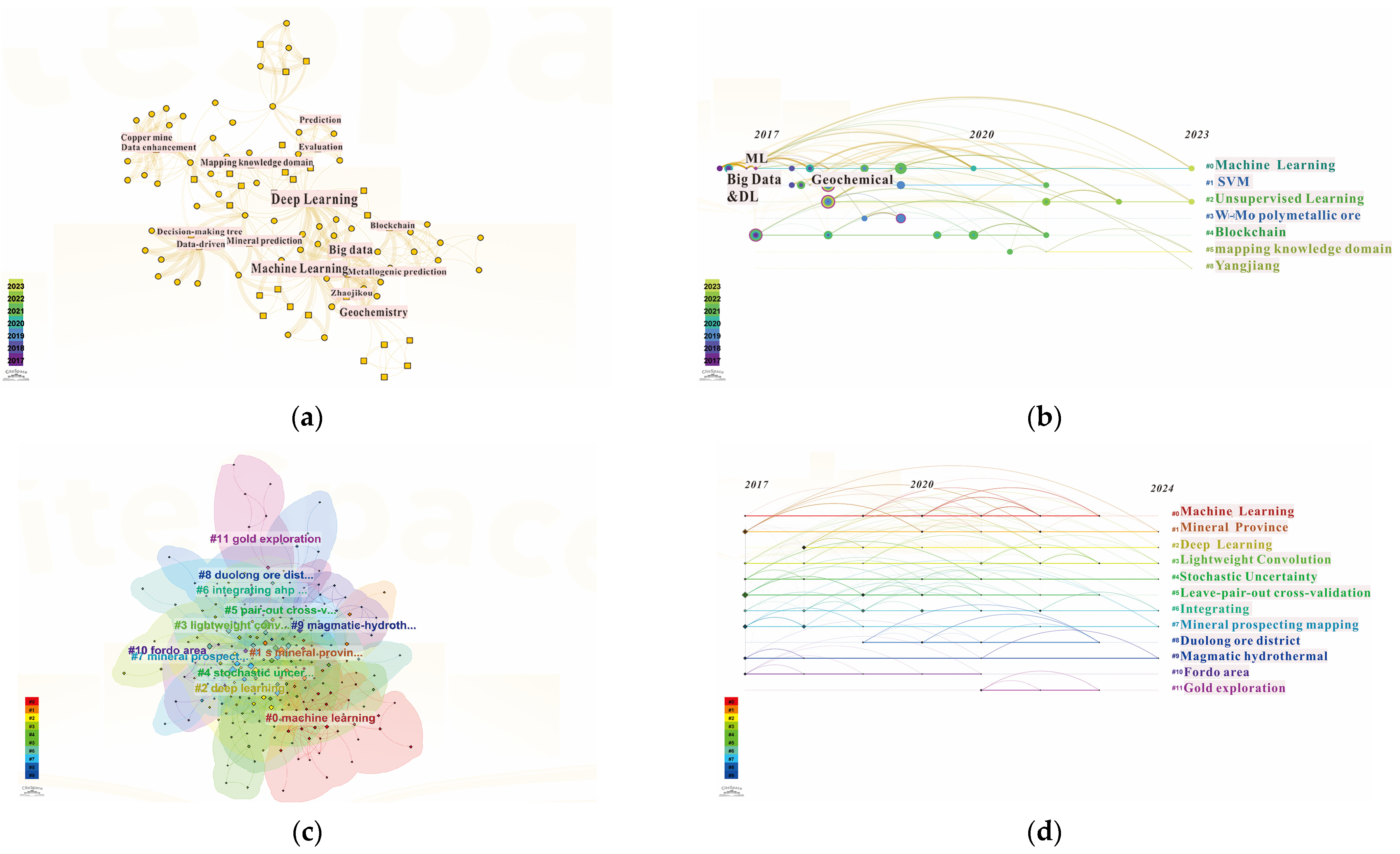

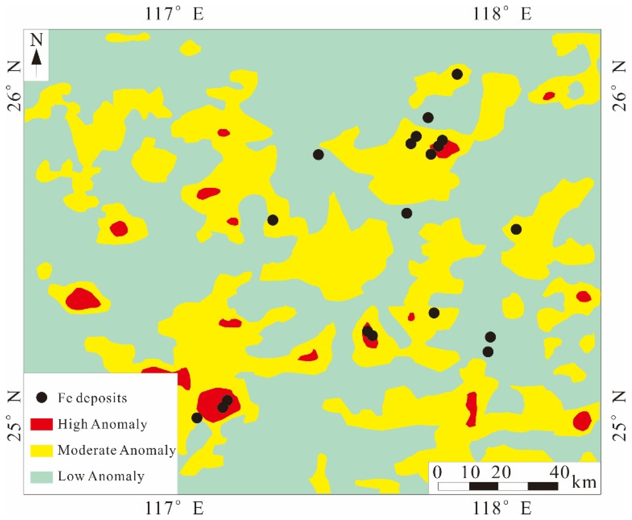
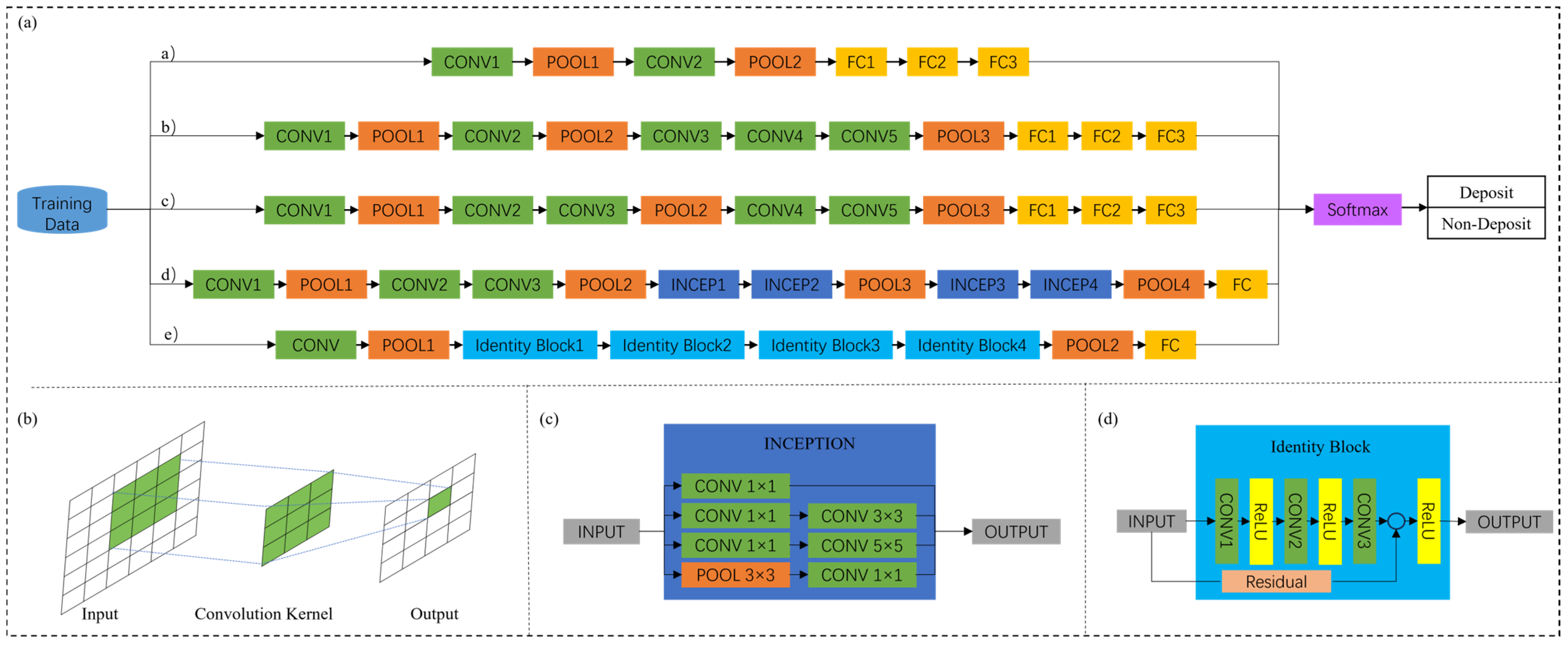
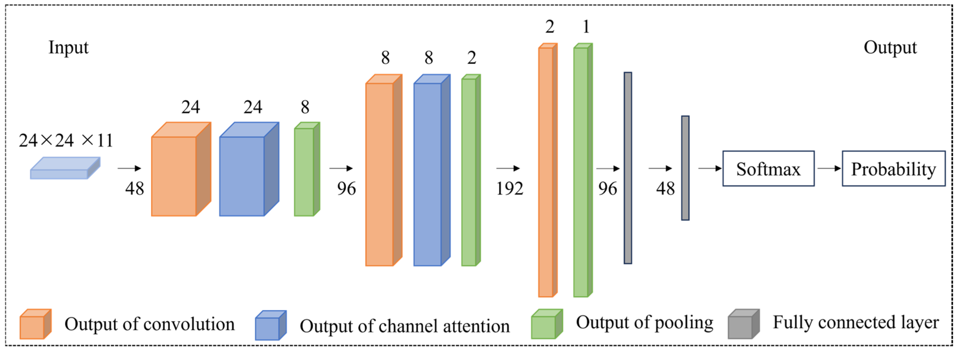
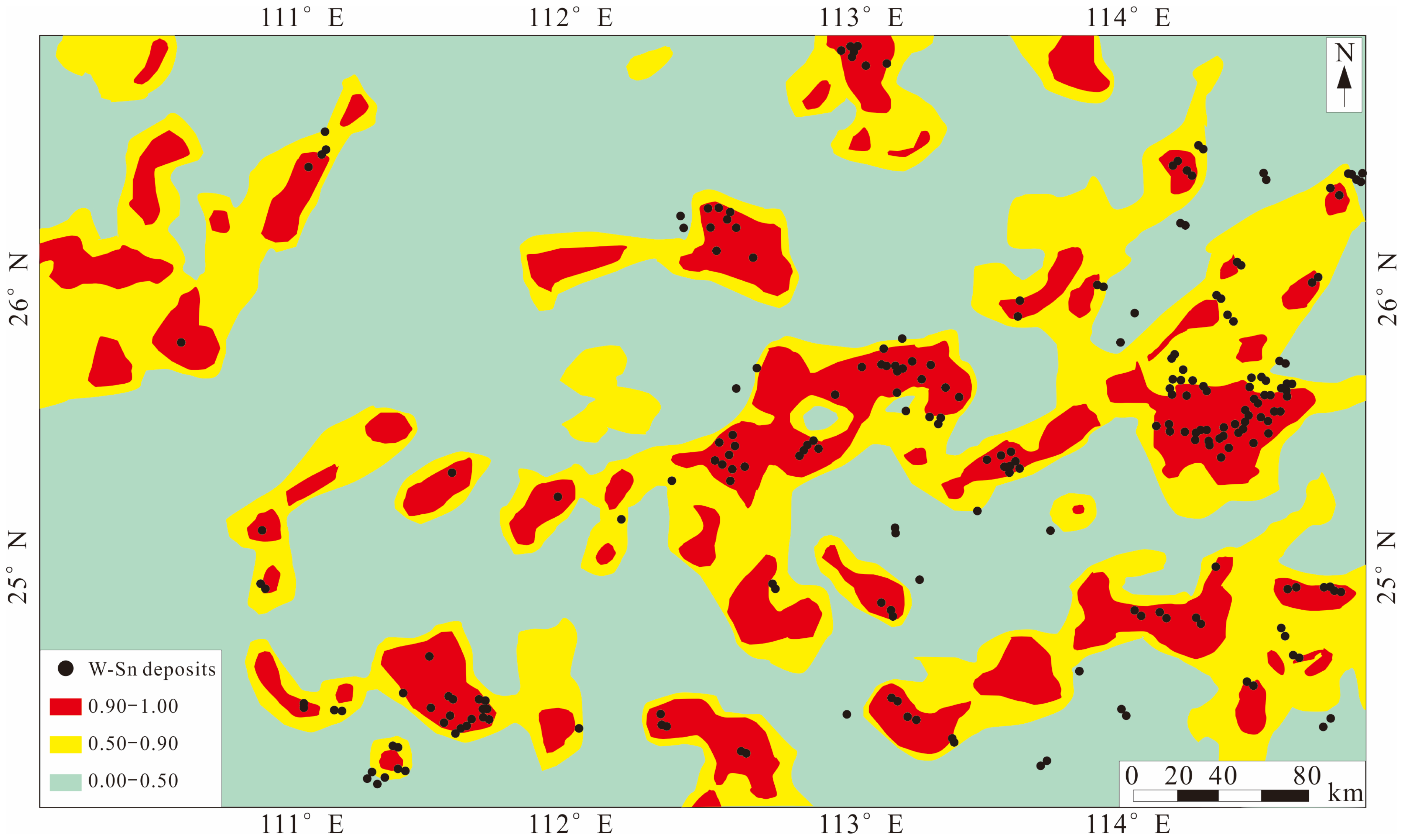
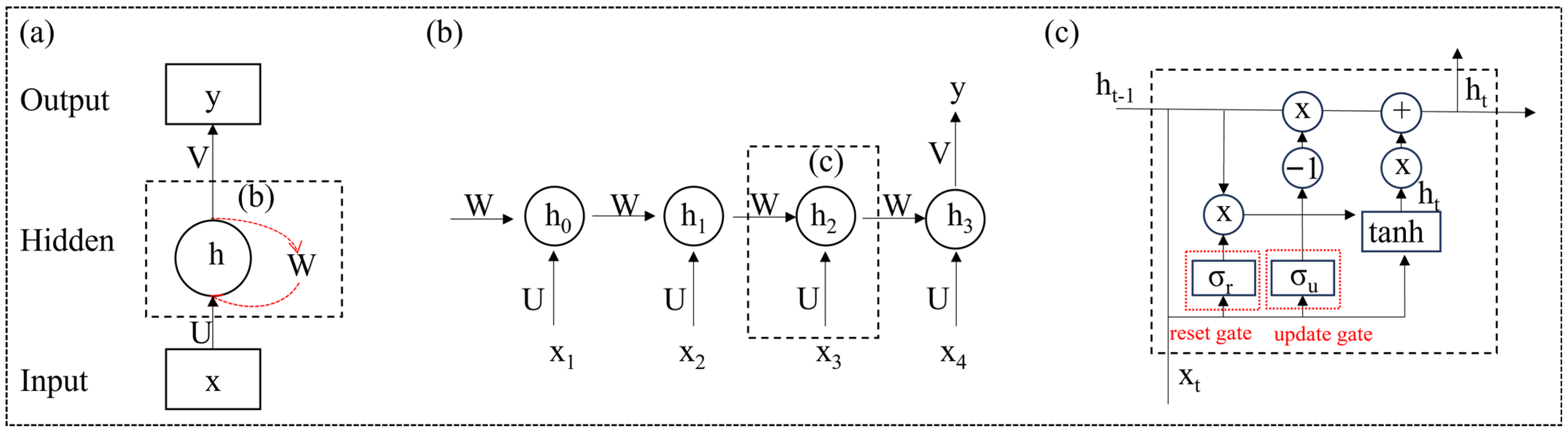
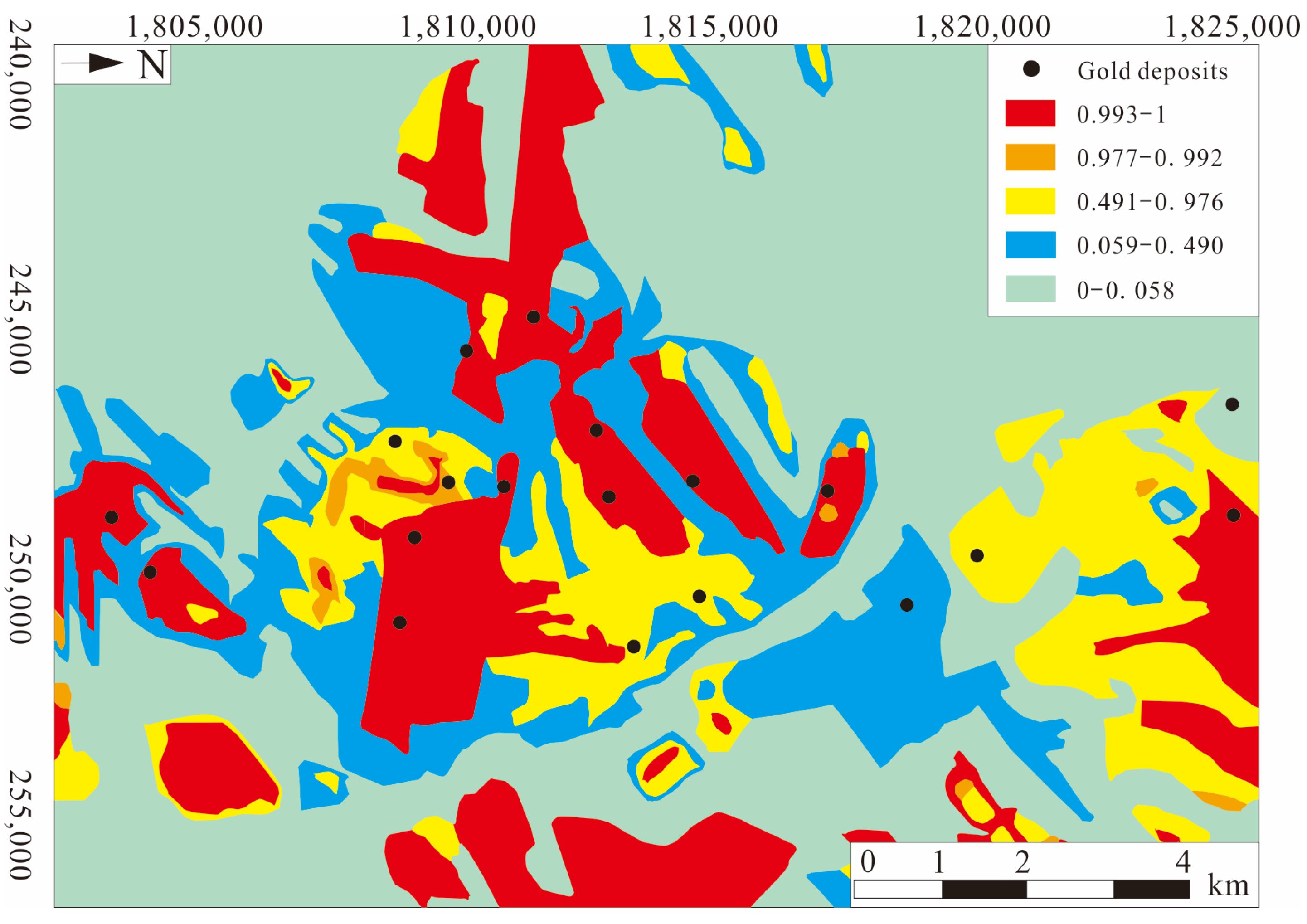
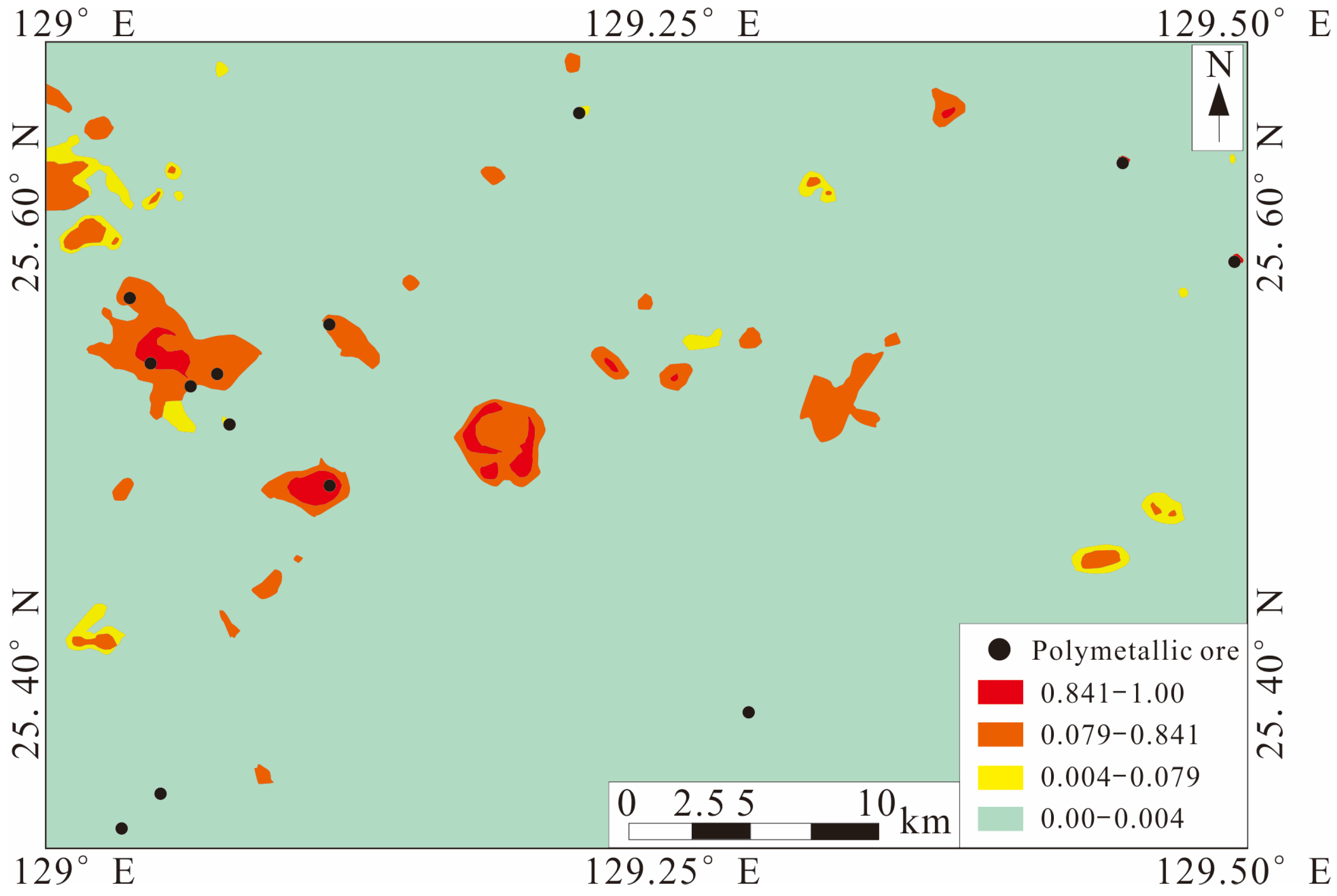
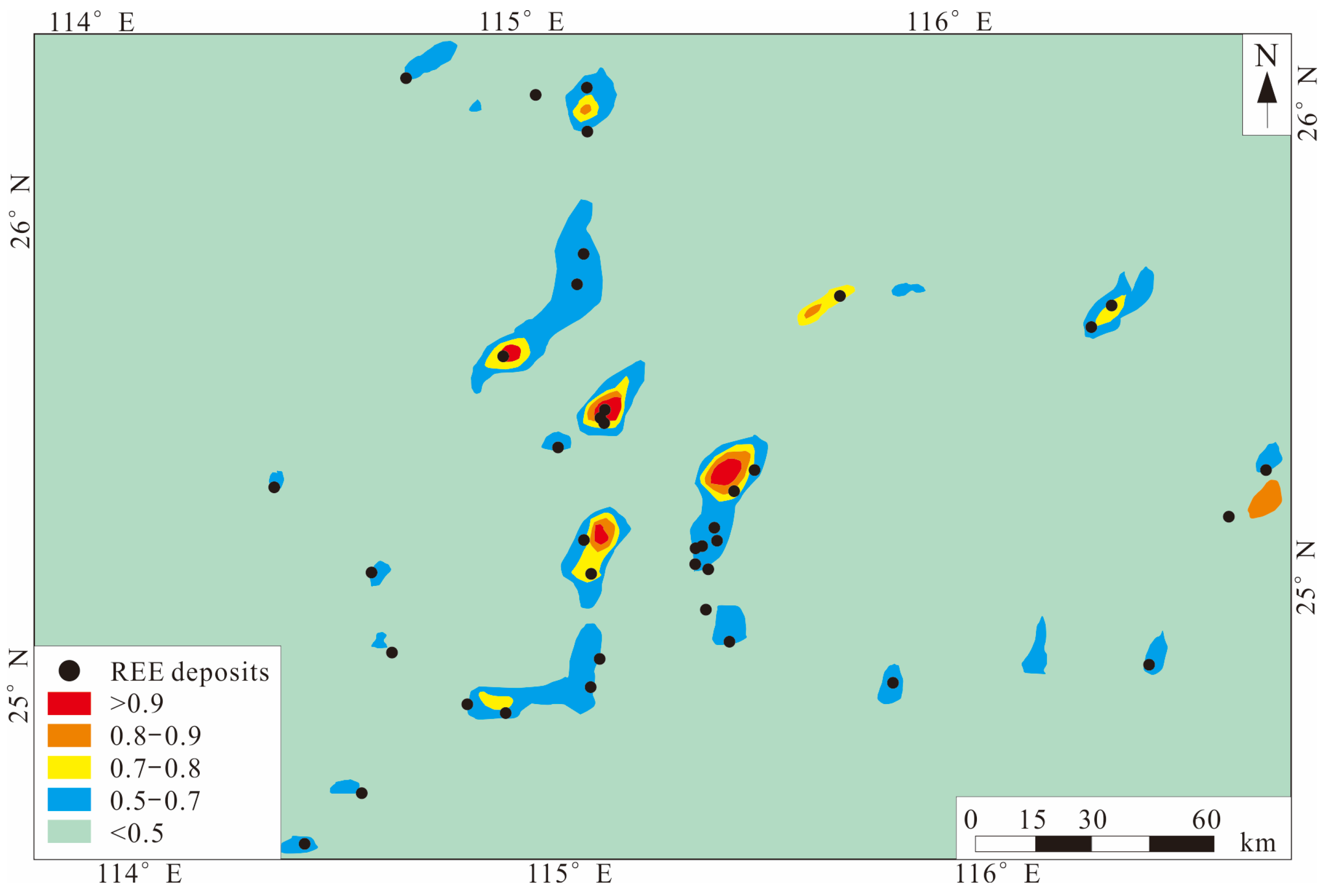
Disclaimer/Publisher’s Note: The statements, opinions and data contained in all publications are solely those of the individual author(s) and contributor(s) and not of MDPI and/or the editor(s). MDPI and/or the editor(s) disclaim responsibility for any injury to people or property resulting from any ideas, methods, instructions or products referred to in the content. |
© 2024 by the authors. Licensee MDPI, Basel, Switzerland. This article is an open access article distributed under the terms and conditions of the Creative Commons Attribution (CC BY) license (https://creativecommons.org/licenses/by/4.0/).