Insights on Determining Improved Conditions for Multipurpose Reagent Dosing to Increase Froth Flotation Efficiency: NaSH in Cu-Mo Selective Flotation Case Study

Abstract

The assessment of mineral surface hydrophobicity at the industrial scale is a challenge. In some industrial situations, such information is indirectly obtained from other proxy variables. A well-known example of this is observed in the Cu-Mo selective flotation operation, where sodium hydrosulphide is used to change the redox potential and, controlling this value, determine when Cu-sulphide floatability is inhibited. Preliminary experiments indicate that this reagent may also promote the formation of solid precipitates, reducing its impact on the redox potential. This study aims at designing a simple strategy at the laboratory scale to report and quantify NaSH losses due to parallel, irreversible, and/or fast reactions, such as precipitation. Experiments carried out using process water coming from a Cu-Mo selective flotation plant in Chile show that departing from different pH conditions and the addition of hydrosulphide ions effectively triggers the precipitation of specific metal ions, decreasing its availability to reduce the redox potential of the aqueous solution. For this specific case scenario and water quality, around 5% of the NaSH dosed precipitated. An SEM-EDX analysis of the produced solid phase shows that it is composed of mainly iron sulphide and hydroxide, along with other metal hydroxides. More importantly, it was found that dosing the reagent at the same concentration, but in the form of small increments, allows reaching the redox potential more efficiently, reducing to some extent the precipitate production and the unnecessary NaSH consumption in up to 30% of the NaSH dosed. Preliminary 1-D modelling of the process, based on mass transport coupled with reaction mechanisms, provided a first indication of the best dosing conditions for this reagent. The latter is expected to contribute to the development of better and improved reagent dosage technologies in froth flotation environments.

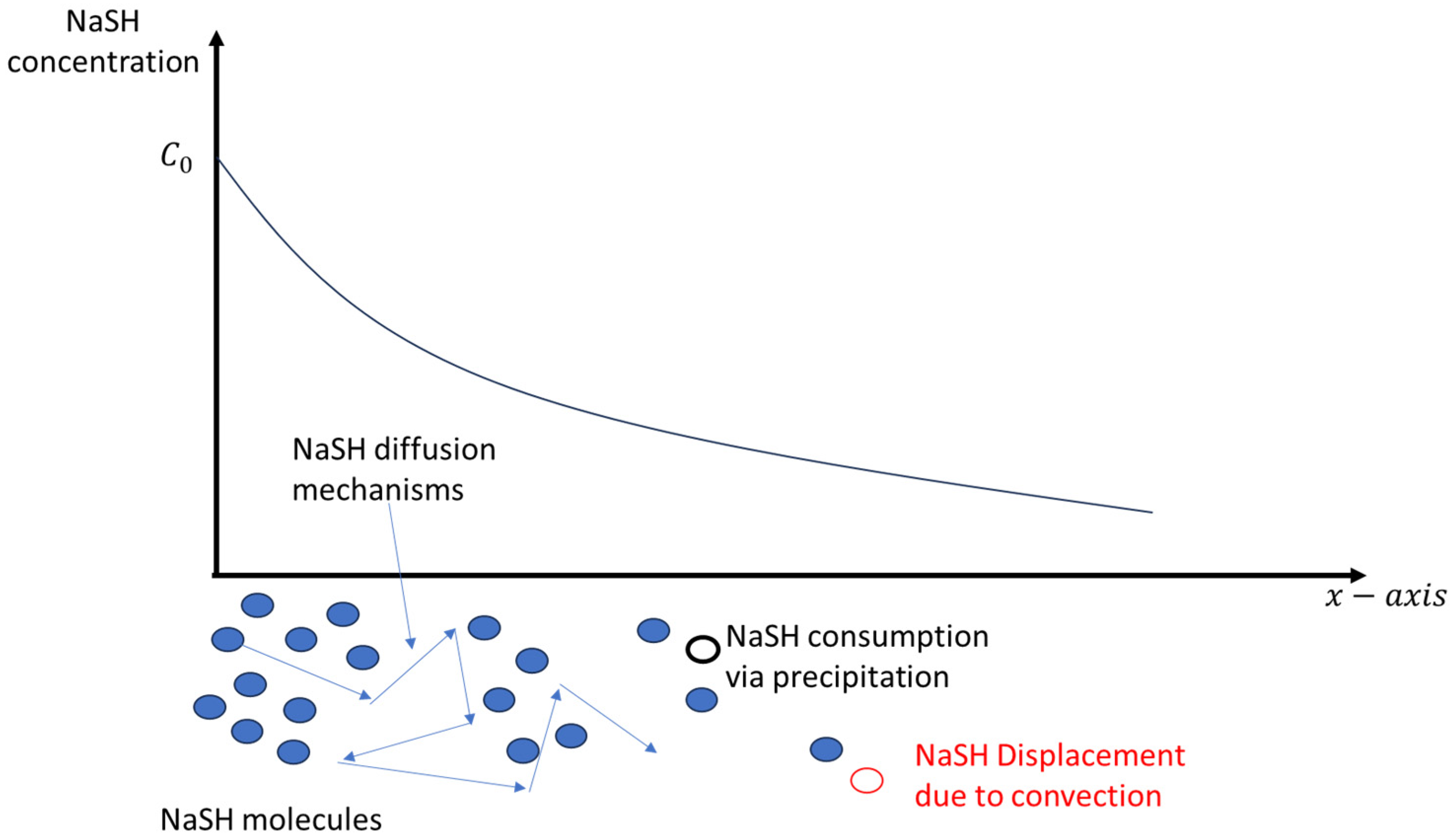
1. Introduction

After more than 100 years of history, froth flotation remains one of the most versatile yet complex processes to understand [1]. Outcomes of research studies do not only depend on the subprocess chosen or the specific perspective addressed but also, as many researchers have pointed out, on the scale used in the study [2,3,4]. On one hand, it is undeniable that much of the progress accomplished by understanding how froth flotation works comes from the direct measurements performed during plant surveys originally proposed by D.F. Kelsall [5]. On the other hand, fundamental knowledge produced at the laboratory scale has also provided significant insights on different subprocesses. However, when looking at the scientific literature, the leap between the knowledge achieved at a small scale and that accomplished at industrial looks, in many aspects, almost insurmountable. The chemistry involved in the separation process is not an exemption of this situation [6,7]. Significant effort has been put towards understanding the chemistry behind the selectivity of flotation separations [8,9,10], and researchers working with laboratory tests have struggled to procure answers that could be effectively applicable into larger scales. For instance, one facet that has not been assessed thoroughly, is whether the location and the rate at which a reagent is being dosed would have an impact on the process efficiency. Indeed, the dosing of a reagent at large scale is often performed using high concentrations and choosing convenient locations within the flotation tank expecting fast mixing, quick dispersion, and/or dilution and other almost instantaneous effects. At the laboratory scale, mechanisms associated with the homogenisation of the reagent in the aqueous/pulp phase are particularly much quicker than that at the industrial scale, since the power input per unit of volume is high [11,12], while at the industrial scale, a mass transfer phenomena increases the difficulty to understand the efficiency of many subprocesses, and therefore, that of the overall process. The latter, coupled with the fact that reagents may have more than one role in froth flotation, makes this situation even more difficult to understand. This study aims at addressing these challenges following to some point “the divide and conquer strategy”, using sodium hydrosulphide (NaSH) as an example and the Cu-Mo selective flotation as the specific application.

In the case of many Cu-Mo flotation plants, at early stages of Mo-selective flotation circuit, both NaSH and sulphuric acid (H₂SO₄) are used to decrease the hydrophobicity of copper–sulphide minerals, enhanced in the previous stage of the Cu-Mo collective flotation circuit, with good results. In many flotation plants, sulphuric acid is dosed first, and sodium hydrosulphide is dosed afterwards. Both reagents are not particularly compatible chemistry wise, as they would produce hydrogen sulphide gas. To sort this out, most of the plants dosing both reagents work with sealed flotation cells in the selective flotation circuit. These two reagents, primary considered bulk active rather than surface active, after being dosed, would be firstly transported across the aqueous phase and, simultaneously or afterwards, it is expected that they would react with the surface of mineral particles removing, to a certain extent, the surface hydrophobicity of copper sulphides minerals.

NaSH is commonly dosed at the industrial grade in the aqueous form at 42% (density: 1.3 g/mL, 20 °C). From a chemical reaction point of view, the reagent primary develops the reaction equilibria represented by Equations (1)–(3):

$$Na{SH}_{\left(s\right)}\leftrightarrow {Na}_{\left(aq\right)}^{+}+{HS}_{\left(aq\right)}^{-}$$

(1)

$$H_2{S}_{\left(g\right)}+2H_2{O}_{\left(l\right)}\leftrightarrow H_3{O}_{\left(aq\right)}^{+}+{HS}_{\left(aq\right)}^{-}$$

(2)

$${HS}_{\left(aq\right)}^{-}+2H_2{O}_{\left(l\right)}\leftrightarrow H_3{O}_{\left(aq\right)}^{+}+S_{\left(aq\right)}^{2-}$$

(3)

Furthermore, when enquiring the scientific literature about the impact of this reagent in froth flotation operations, several different effects are pointed out, such as:

(a)

Deactivating or depressing the hydrophobicity of copper-bearing sulphide minerals in molybdenum selective froth flotation when reaching redox potential ranging between –400 mV and –600 mV vs Ag/AgCl [13,14,15];

(b)

Reducing the pulp potential to avoid accidental over-oxidation of the mineral [16];

(c)

Changes in froth stability [17];

(d)

pH control [18];

(e)

Sulphidisation of metal oxides [19].

All of these multiple effects suggest that, in the worst-case scenario, simultaneously competing chemical reactions and other physical processes and subprocesses would occur during the selective mineral separation. The latter means that the dosed NaSH could have impacted the system much earlier than it carried out its main purpose of reaching the surface of copper sulphide minerals to decrease its floatability. Indeed, a thermodynamic analysis predicts that to have an impact on the redox potential over a relatively important range of values, the reagent should be in dissolved state and at a concentration ratio between the reduced and the oxidised forms that are relatively significant. Following this line of thought, the possible precipitation of the species would reduce the impact of the reagent dosage on the redox potential, and in that case, it would be important to assess the magnitude of such effect and to identify the strategies to avoid it.

Therefore, this study attempts to gather information about the roles NaSH plays in Cu-Mo-selective flotation plants, which inevitably leads to its overconsumption in other chemical and physical sub-processes, reducing their availability for its main purpose. And, at the same time, this study also attempts to shed light towards how the manner of dosing this reagent may have a key impact on the multiple roles it may undertake.

2. Materials and Methods

2.1. Eh and pH Monitoring during NaSH Dosing

A set of three laboratory tests were carried out to study the chemistry of NaSH dosing in process water. The experiments consisted of dosing incremental volumes (3, 6 and 12 mL) of NaSH of technical grade (41.7% mass at pH 12) in 1 L of process water, originally at pH 5.9. These doses are consistent with those reported by various researchers [20,21,22]. The experiments were conducted at 18.9 °C. All of the experiments were performed in triplicate to study the reproducibility. The process water was procured by a mine site located in the northern part of Chile. The pulp sample coming from a Mo-selective flotation circuit was sampled at a plant location just before dosing the sodium hydrosulphide depressant. The slurry sample was filtered until a crystalline water sample was obtained, to which NaSH was dosed.

Throughout the experiments, the redox potential (Eh) and pH were continuously monitored and registered. NaSH dosing was sequentially performed, and each dose was added after the stabilisation of the pH and the redox potential was achieved. The experiments timespan was designed to take no longer than 120 s. The experiments ended once reaching –480 mV vs SCE (the potential threshold used by the mine site from which the process water was sampled). All tests were performed in triplicate and the average values are presented. The uncertainty of the variables observed in the experiments are presented. All of the redox potential results are reported versus a calomel standard electrode (SCE), unless said otherwise.

2.2. NaSH Dosing Tests Leading towards Precipitate Characterisation

A set of three laboratory tests were carried out to study the chemistry of NaSH dosing in aqueous solutions departing from different pH conditions. To promote the formation of precipitates, the experiments consisted of dosing 40 mL of NaSH of technical grade (41.7% mass at pH 12) in 1 L of process water, originally at pH 5.9, but conditioned at pH 6, 8, and 10. The pH modifier used was sodium hydroxide. In the case that precipitates appear after dosing NaSH, the solids were separated by ultracentrifugation at 2000 rpm for 20 min in a Sorvall RC-5B refrigerated Superspeed Centrifuge, Thermo Fisher Scientific, Santiago, Chile, followed by a filtration stage using Filter Advantec No. 03, McMetodos de Control S.A., Buenos Aires, Argentina. The solids were dried in an oven at 30 °C overnight. Then, they were submitted to a Field Emission Scanning Electron Microscope coupled with Energy Dispersive X-ray Spectroscopy (FE-SEM-EDX) analysis GeminiSEM 360, with a Gemini 1 optic InLens detector, Carl Zeiss AG, Oberkochen, Germany, which ensures an efficient signal detection for both secondary (SE) and backscattered (BSE) electrons, while the EDX was performed using an Ultim Max 40 detector (OXFORD Instruments, High Wycombe, UK) to carry out elemental analysis on the particles surfaces.

3. Results

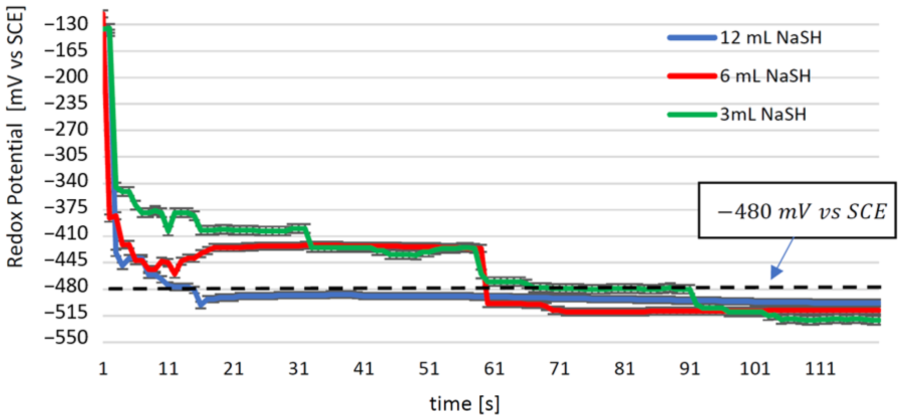
3.1. Eh and pH Monitoring during NaSH Dosing

Figure 1 shows the redox potential results with time when adding different increment of NaSH doses to the process water. Firstly, regarding the uncertainty observed in the redox potential measurements during the first 10 s of the experiment, the steep decrease in the measured voltages lead to uncertainties that can be as high as 42%, expressed as the coefficient of variation, which can be associated with the mixing and mass transport phenomena. However, the results were highly reproducible when the redox potential stabilised (relative error below 2%) which secured the robustness of the results. In terms of redox potential behaviour, as expected, when dosing 12 mL of NaSH, the redox potential decreased until reaching a value of about −491 mV. When dosing the 12 mL in two stages, each one made of 6 mL, the redox potential reduction was not linear. After adding the first dose, the redox potential reduced and stabilised at around −420 mV. After adding the second 6 mL, the redox potential reached was about −510 mV; 20 mV lower than that observed when dosing 12 mL at once. If the 12 mL dosage is divided in four doses of 3 mL, the redox potential is achieved only using three out of four doses, reducing the NaSH consumption by 25%. Or, in other words, one unit of NaSH would be replaced by 75% of that same unit producing the exact same effect on redox potential, meaning an increase of 33%.

This attenuated behaviour of the redox potential when adding the reagent in smaller doses but in several times can be explained by the fact that in the Nernst equation, for each one of the two major half-reactions, the impact of the concentration appears in the argument of the logarithmic function (Equation (4)):

$$E=E^0+\frac{0.0591}{n}ln\frac{a_i^{\left(OX\right)}}{a_i^{\left(RED\right)}}$$

(4)

where $E$ is the equilibrium potential, $E^0$ is the standard equilibrium potential, $n$ is the total number of electrons being transferred in the reaction, and $a_i^{\left(OX\right)}$ and $a_i^{\left(RED\right)}$ represent the activity or the real concentration of the oxidised and reduced species, respectively, participating in the reaction.

From a kinetic standpoint, the redox potential always follows the mixed potential, if the electrical conductivity of the electrode substrate makes it possible (which in the case of the Eh probe holds) [23]. The irreversible electrochemical theory indicates that this behaviour is also governed by the electrochemical reversibility of each of the redox reactions involved [24,25], which in this case it would be an anodic control [26].

Figure 2 shows the pH variations during the experiments. Probably due to the fact that the experiment timespan is in the order of the time response of a pH-meter [27], especially in the case of the four doses, this variable shows a more instable behaviour than the redox potential exhibiting coefficients of variation between 18% and below 0.07%. The pH increases with the dosing of NaSH, as the reagent is dosed in an aqueous solution at a pH close to 12. Similar to the response of Eh, the dosing of NaSH in one dosage increases the pH up to about 8.5. When splitting the dosage in two, the pH reached a similar value. And when splitting into four doses, the pH raises only up to 7.6. This behaviour can be explained as the use of ${OH}_{\left(aq\right)}^{-}$ groups in the formation of metal hydroxides (Equation (5)) [28]:

$$M_{\left(aq\right)}^{n+}+{nOH}_{\left(aq\right)}^{-}\leftrightarrow {M\left(OH\right)}_n$$

(5)

where the most relevant reaction found in the present study would be $M\equiv Fe$ and $n=2$.

This response may reflect the buffering capacity of the process water or the formation of compounds that restrict pH increase, such as the precipitation of metal sulphides [29].

The mass balance of ${OH}_{\left(aq\right)}^{-}$ becomes a difficult task since non-idealities take place at such a high pH value [30]. Notwithstanding the latter, it can be suggested that other mechanisms to neutralise the alkalinity of the reagent may take place. At pH 11.2, mostly every metal will experience, to some extent, a certain hydrolysis. For instance, the reaction of a di-valent metal partially hydrolysed is shown in Equation (6):

$${MOH}_{\left(aq\right)}^{-}+{HS}_{\left(aq\right)}^{-}\leftrightarrow {MS}_{\left(s\right)}+H_2{O}_{\left(l\right)}$$

(6)

For the case of iron, the $∆G^0$, $∆H^0$, and $∆S^0$ are $-18.14 \mathrm{k}\mathrm{c}\mathrm{a}\mathrm{l}/\mathrm{m}\mathrm{o}\mathrm{l}$, $-2264.13 \mathrm{k}\mathrm{c}\mathrm{a}\mathrm{l}/\mathrm{m}\mathrm{o}\mathrm{l}$, $7.65 \mathrm{k}\mathrm{c}\mathrm{a}\mathrm{l}/\left(\mathrm{m}\mathrm{o}\mathrm{l}\mathrm{K}\right)$, respectively [31,32]. With these values ($K=2.027\times {10}^{13}$—mostly products species present at the equilibrium), the redissolution would be thermodynamically challenging in these conditions. This behaviour could also be extended to surface hydroxyl groups, as shown in Equation (7):

$$\equiv MOH+{HS}_{\left(aq\right)}^{-}\leftrightarrow {\equiv MS}_{\left(s\right)}+H_2{O}_{\left(l\right)}+1e^{-}$$

(7)

where $\equiv MOH$ represents a metal oxide site at a mineral surface and ${\equiv MS}_{\left(s\right)}$ is a sulphide site formed. Interestingly, the stoiquiometry indicates that the presence of an oxidant might be required to achieve the sulphidation. A simple exploration of the stoichiometry of reaction 7 taking place with a fully alkaline ionised oxide surface site ($\equiv M{O}^{-}$) increases the number of electrons being transferred, but it would not explain the neutralisation of hydroxyl ions. The mechanism of the same reaction with sulphide ions ($S_{\left(aq\right)}^{2-}$) is more complicated from a stoichiometric standpoint.

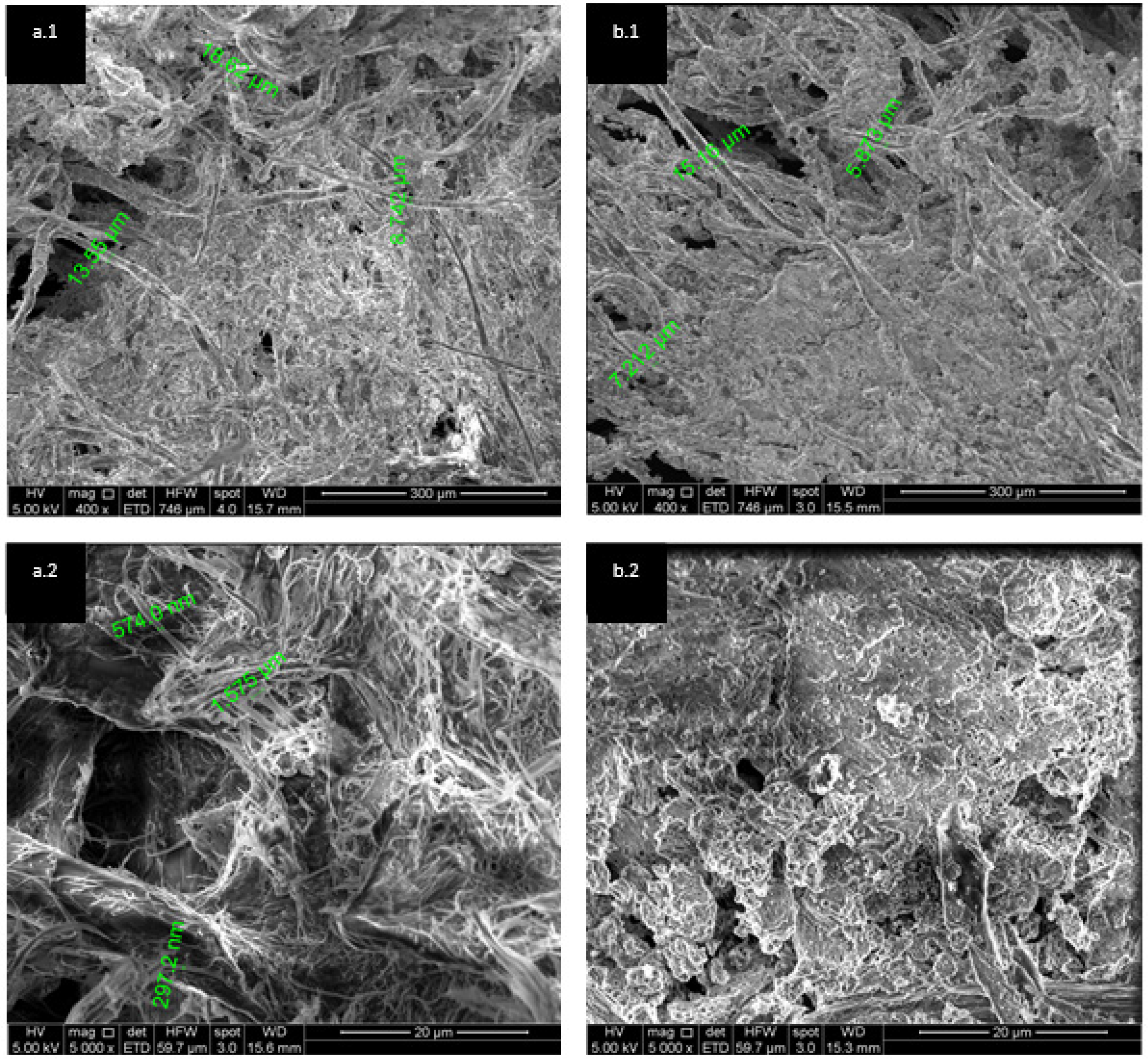
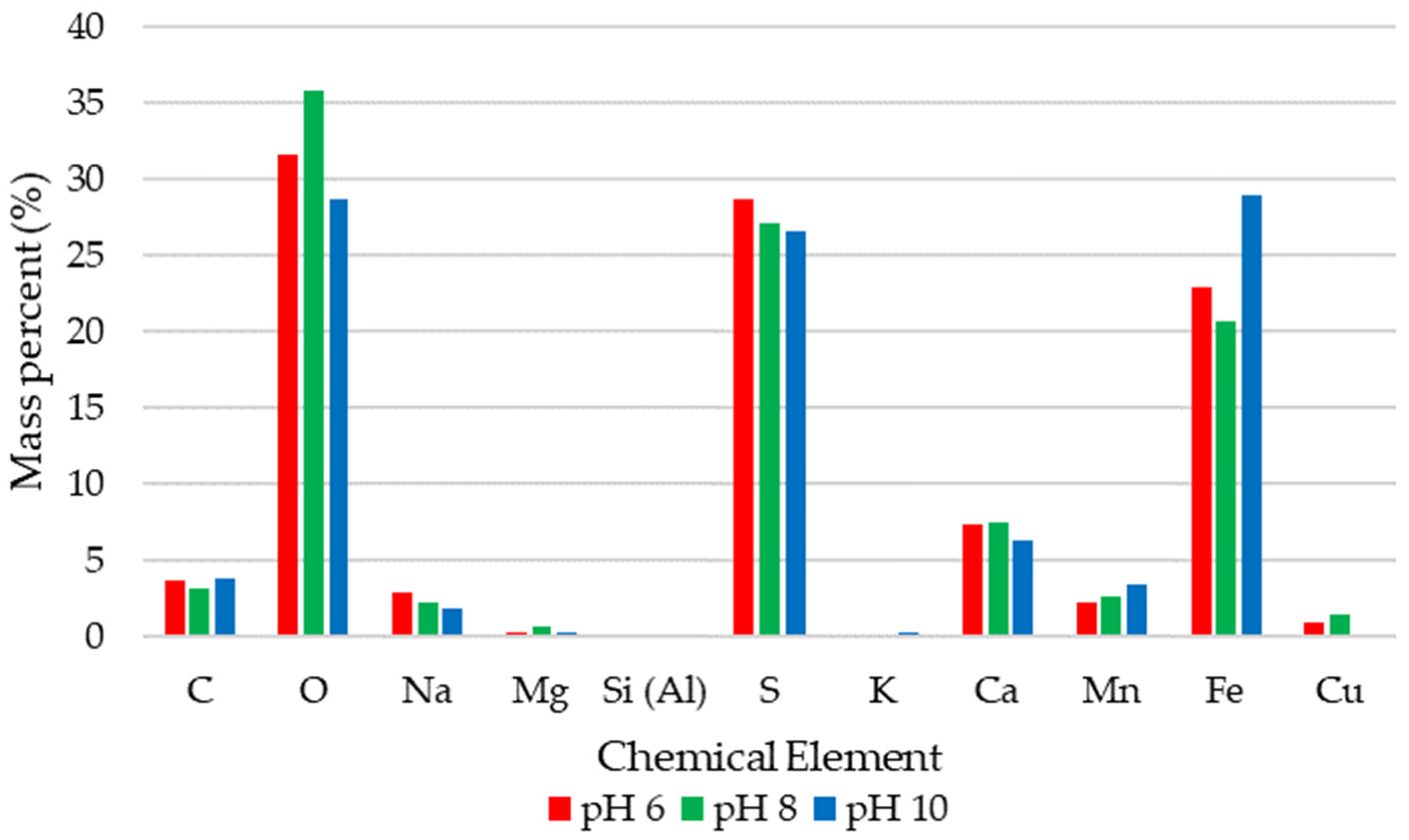
3.2. Test B. Precipitate Characterisation

When dosing the reagent NaSH into the plant water, the water turns dark black. A precipitate is being formed. Therefore, a fraction of the dosed NaSH is not being used to reduce the redox potential of the aqueous phase but is used instead to form a precipitate.

Although the speciation diagrams at the working pH range show the predominance of the sulphide ion species at pH 11.2 is ${HS}_{\left(aq\right)}^{-}$, and the equilibria with other forms of the ion represented by Equations (1)–(3) are almost instantaneously reached, and notably with $S_{\left(aq\right)}^{2-}$ nearly three units of pH apart, to form metal sulphide precipitates.

Figure 3 shows SEM pictures of the precipitate when the NaSH dosage is performed at pH 6, 8, and 10.

Appendix A details the specifics of the SEM analysis. At pH 6, fibre-like precipitate is observed and is probably associated with iron oxy-hydroxide structures [33]. The fibres thickness range between a few hundred nanometres and up to 18 μm. At pH 8, fibres still appear, but their diameters appear in a narrower range (from a few micrometres up to 15 μm). Additionally, amorphous structures also can be identified, especially when zooming in, and are probably linked to other metal hydroxides [34]. At pH 10, thick fibres are spotted again, similar to pH 8, but at 5000x magnification, an amorphous structure is again observed. Figure 4 shows the chemical analysis of the precipitate formed.

Figure 4 shows the EDX analysis. There is no significant trend in terms of elemental composition when moving from pH 6 to pH 10 in producing the precipitates. The precipitates are formed from the oversaturation of the concentration of metals, sulphide, and hydroxyl groups. Looking at the solubility product constants, the most relevant species for this case study are structures like ${FeS}_2$, $FeS$, $CaS$, $MnS$, $Fe{\left(OH\right)}_2$, $Ca{\left(OH\right)}_2$, and $Mn{\left(OH\right)}_2$. Considering these species, an educated guess was made by minimising the element content between the experimental results and that provided by the mentioned structures. The best adjustments were obtained when considering iron and other metals hydroxides and neglecting the $FeS$-like structure, which agrees with the Pourbaix diagrams of iron–oxygen and iron–sulphur–oxygen (Figure 5). For a matter of exemplification, only relevant iron-bearing Pourbaix diagrams are shown.

The reaction equilibria take place rapidly, as most of the sulphide ions are introduced in the system in the form of hydrosulphide, and this species in equilibrium with sulphide ions immediately produces insoluble metal sulphides. This result is not in any way striking, as the hydrometallurgy predicts small solubility product constants of metal sulphide complexes. Computations indicate that around 7% of the sulphur effectively dosed is transferred to the solid phase produced by precipitation. The latter means that around 30% of the NaSH dosed is, in this case, used in metal precipitation and reagent excess.

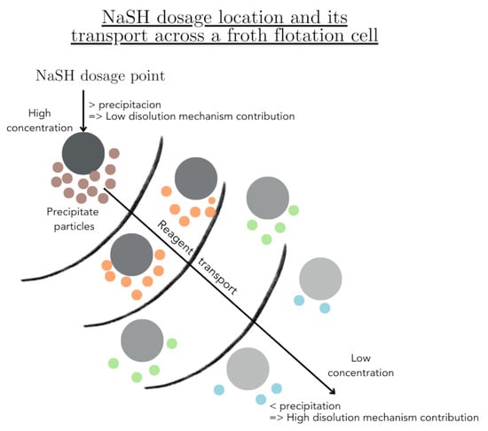
3.3. Modelling and Discussion

3.3.1. Thermodynamics

Using a classic thermodynamic approach, the minimum concentration of NaSH to be dosed without precipitation can be computed.

Commonly the major reactions are those presented in Equations (8)–(16) in

Table 1. Major reactions taking place during NaSH dosage leading to metal precipitation in the form of oxides and sulphides.

$2H_2{O}_{\left(l\right)}\leftrightarrow H_3{O}_{\left(aq\right)}^{+}+{OH}_{\left(aq\right)}^{-}$	$K_w$	(8)
${NaSH}_{\left(aq\right)}\leftrightarrow {Na}_{\left(aq\right)}^{+}+{HS}_{\left(aq\right)}^{-}$	$K_0$	(9)
$H_2{S}_{\left(g\right)}+H_2{O}_{\left(l\right)}\leftrightarrow H_3{O}_{\left(aq\right)}^{+}+{HS}_{\left(aq\right)}^{-}$	$K_1$	(10)
${HS}_{\left(aq\right)}^{-}+H_2{O}_{\left(l\right)}\leftrightarrow H_3{O}_{\left(aq\right)}^{+}+S_{\left(aq\right)}^{2-}$	$K_2$	(11)
$M{S}_{\left(s\right)}\leftrightarrow M_{\left(aq\right)}^{2+}+S_{\left(aq\right)}^{2-}$	${Kps}_{\left(1\right)}$	(12)
$M{S}_{\left(s\right)}+S_{\left(aq\right)}^{2-}\leftrightarrow {MS}_{\left(aq\right)}^{2-}$	$K_3$	(13)
$M_{\left(aq\right)}^{2+}+2H_2{O}_{\left(l\right)}\leftrightarrow {MOH}_{\left(aq\right)}^{+}+H_3{O}_{\left(aq\right)}^{+}$	$K_h$	(14)
$M{\left(OH\right)}_2\leftrightarrow M_{\left(aq\right)}^{2+}+2{OH}_{\left(aq\right)}^{-}$	${Kps}_{\left(2\right)}$	(15)
$M{\left(OH\right)}_2+H_2{O}_{\left(l\right)}\leftrightarrow {M\left(OH\right)}_3^{-}$	$K_4$	(16)

.

These computations assume the instantaneous solubilisation of the NaSH when introduced into a flotation cell and can be estimated using the classic equilibrium type equations.

$$\frac{{Kps}_{\left(1\right)}}{\left[M^{2+}\right]}=\frac{{\left[M^{2+}\right]}_0}{1+K_3+\frac{{\left[{H_{3}O}^{+}\right]}^2}{K_1{K}_2}+\frac{\left[{H_{3}O}^{+}\right]}{K_2}}$$

(17)

$$\frac{{Kps}_{\left(2\right)}}{\left[M^{2+}\right]}=\frac{{\left[M^{2+}\right]}_0-\frac{K_3^{*}}{\left[{H_{3}O}^{+}\right]}}{1+\frac{K_1^{*}}{\left[{H_{3}O}^{+}\right]}+\frac{K_3^{*}{K}_4^{*}}{{\left[{H_{3}O}^{+}\right]}^2}}$$

(18)

where the Equations (17) and (18) represents the maximum metal concentration in the aqueous solution without triggering precipitation for metal sulphide (neglecting sulphide complexes above mono-coordinated) and metal hydroxide, respectively. As expected, the lower the concentration of hydronium ions, the higher the chances of appearing hydroxides.

This can be solved for each pH using the condition of electroneutrality (Equation (19)).

$$\sum _{i=1}^{n}l\left[X_i^{+l}\right]=\sum _{j=1}^{m}k\left[X_j^{-k}\right]$$

(19)

In this case, it is difficult to know the exact concentration of all the species present in the system and it can be quite laborious task when considering real concentrations. Furthermore, this analysis could be misleading, as to avoid oversaturation it might be concluded that the reagent should be dosed at a very low concentration, which is impractical. Indeed, since the solubility product constants of some of the metal sulphides are very low [37], so to avoid precipitation the reagent concentration should be extremely diluted in the aqueous phase, reducing its activity to undertake any further chemical reaction.

3.3.2. Conservation Equations

Another possible way to explain the situation involves applying the equations of classic mass transport coupled with chemical equilibria [38]. The latter would highlight that the chemical reactivity of the reagent, its state of aggregation, and the way it is dosed are all equally relevant.

In practical terms, there is a reagent dosed in a dissolved state which diffuses reducing its concentration, as it is transferred enabling the reduction of the redox potential (and then reducing the floatability of copper sulphide minerals). Simultaneously there are other mechanisms also reducing its concentration through oversaturation, producing solids (Figure 6 left, right-hand side). At the dosing point, the concentration of NaSH is at its highest level promoting the formation of the precipitates and once being transported throughout the system, its concentration decreases and so does its tendency to produce solids.

Figure 7 shows a schematic of the reagent depletion as it is transferred across the system. Assuming that the chemical equilibrium takes place in the real system quickly and that the reverse reaction is unlikely to occur. Also, considering 1D model, the reagent could be decreasing its concentration at a specific point due to displacement in the space, due to convective mechanisms. In other words, the present model presumes that once an amount of NaSH, either by parallel reaction or transport mechanisms, is reduced, it will remain as so.

Considering the conservation equation of a specie “$i$” (NaSH regent) dosed at a specific location of a pulp phase [38]:

$$\frac{\partial c_i}{\partial t}+\nabla \left(c_i{\overrightarrow{v}}_i-D_i\nabla c_i\right)=R_i$$

(20)

where $c_i$ is the concentration of the reagent, $v_i$ is the fluid velocity (assuming that the reagent is dosed in a moving liquid, such velocity becomes the velocity of the fluid), $D_i$ is the diffusion coefficient of the reagent in the dissolved state, $R_i$ is the reaction rate (in this case, of consumption whenever the reagent leads to salt precipitation), and $t$ represents the time. Considering that in froth flotation, the fluid where the reagents are dosed is incompressible, then, it will be divergence free, and Equation (21) is obtained:

$$\frac{\partial c_i}{\partial t}+{\overrightarrow{v}}_i\nabla ·c_i-D_i{\nabla }^2{c}_i=R_i$$

(21)

In steady state conditions, the dosing of the reagent in aqueous phase is characterised by a constant flow rate (constant concentration at the dosing point):

$${\overrightarrow{v}}_i\nabla ·c_i-D_i{\nabla }^2{c}_i=R_i$$

(22)

Equation (22) for 1-D system writes as Equation (23):

$${\overrightarrow{v}}_x\frac{\partial c_i}{\partial x}-D_i\frac{{\partial }^2{c}_i}{\partial x^2}=-k{c}_i^n$$

(23)

The Equation (23) can be translated into scaling estimates as Equation (24) [39]:

$$\frac{v}{\delta }-\frac{D}{{\delta }^2}=-k{c}_0^{n-1}$$

(24)

where, $c_0^{n-1}$ represents the difference between the actual concentration of the reagent and the concentration at the saturation point, or ${\left(c-c_{sat}\right)}^{n-1}$.

The physical length reached by the reagent before any of the two mechanisms reducing its concentration take place is as follows:

$$\delta =-\frac{v}{2k{c}_0^{n-1}}+\sqrt{{\left(\frac{v}{2k{c}_0^{n-1}}\right)}^2+\frac{D}{k{c}_0^{n-1}}}$$

(25)

Rearranging the argument in the squared root, Equation (26) is obtained:

$$\delta =\frac{v}{2k{c}_0^{n-1}}\left[\sqrt{1+\frac{4Dk{c}_0^{n-1}}{v^2}}-1\right]$$

(26)

Expanding the squared root and taking only the first three terms, the physical length can be estimated using Equation (27):

$$\delta ~\frac{D}{v}-\frac{D^{2}k{c}_0^{n-1}}{8v^3}$$

(27)

Equation (27) provides an estimation of how far the reagent would move forward in a process water, which can be related to the geometrical length of the flotation tank $L$ following the classic approach to produce dimensionless numbers. The latter leads to Equation (28):

$$\phi =\frac{L}{\delta }={\left(\frac{D}{vL}-\frac{D^{2}k{c}_0^{n-1}}{8v^{3}L}\right)}^{-1}$$

(28)

Looking at the previous relation, it can also be observed that there is a theoretical condition where the physical length goes to zero. This occurs when the Equation (29) holds:

$$v=\sqrt{\frac{1}{8}Dk{c}_0^{n-1}}$$

(29)

This situation is unlikely since it is associated with the conditions where diffusion and convection cancel each other.

More importantly, the physical length at low-reagent concentrations depends directly on the diffusion to fluid convective velocity ratio. The larger the diffusion, the longer the distances the reagent will travel in the system. The same situation is observed in the case where the convection is low. However, the convective velocity in the second term impacts the physical length in the opposite direction. For small convection velocity, the bigger is the second term of the right-hand side of the equation, reducing the physical length. Therefore, there might be an optimum dosage rate for which the physical length is maximised.

The optimum velocity of reagent dosage is established in Equation (30):

$$v=\sqrt{\frac{3}{8}D{k}^{\left(2\right)}{c}_0^{n-1}}$$

(30)

where Equation (30) proves that there might be an optimum dosing range for NaSH, where the physical length reached by the reagent is at its highest. Note that the kinetic rate constant is explicitly written as a second order constant to make the equation physically consistent. Harmandas and Koutsuokos [40] determined the rate of precipitation of iron (II) sulphides from aqueous solutions with $n=2$. The rate of precipitation found was in the order of ${10}^{-8}-{10}^{-5}\frac{mol}{sL}$, with an apparent second order specific velocity constant ranging between 1 and 10 $\frac{L}{s·mol}$. Considering a diffusion coefficient of hydrosulphide ions in the order of ${10}^{-5}$ ${\mathrm{c}\mathrm{m}}^2/\mathrm{s}$ [41], the theoretical velocity that maximises the reaching of the reagent in the system implemented in this study would be approximately 0.02 cm/s. Although it is a small velocity strongly dependent on the diffusion coefficient, it could change, for instance, with temperature, etc.

Other way of looking at these results comes from rearranging Equation (31), where dimensionless terms appear naturally as follows:

$$\phi =\frac{L}{\delta }={\left(\frac{1}{Pe}-\frac{\left\{Da\right\}}{\left\{{Pe}^3\right\}}\right)}^{-1}$$

(31)

or,

$$\phi =\frac{8{Pe}^3}{8{Pe}^2-Da}$$

(32)

where $Pe$ and $Da$ are the dimensionless Peclet and Damkhöler numbers, respectively. It can be observed that, to obtain the minimum $\phi$ it would be necessary to have a Pe number as small as possible.

This is a possible indication that reagents could be more effectively dosed under specific conditions to reach longer distances, reducing its depletion by other mechanisms.

Nevertheless, it is important to note that in any situation where chemical reactions take place improving the effectiveness of a particular reagent the benefit of using a certain excess of the reagent should not be overlooked, as otherwise it could become a limiting factor of the process. Plus, it is important to remember that this is one simplified interaction of the reagent taking place in the pulp system. Particularly, the impact of the presence of solids may also have an important contribution to NaSH consumption.

Novel technologies could take advantages from this result, such as the dosage of regents in the form of chemical complexes that can ionise as they move towards volumes where their concentration is reduced, etc.

This explanation might also be applied to other similar situations where the reagent being dosed undergoes different subprocesses, particularly two; reagent dispersion governed by diffusion and convection, and reagent reaction. For instance, in the case of surface-active reagents, this might be the dispersion of collectors/frothers and simultaneous micelles formation, etc.

4. Conclusions

A simple laboratory scale strategy to test the impact of reagent dosage when dosed to process water was implemented and interpreted.

The selected case study is sodio hydrosulphide. The test allowed us to prove that splitting the reagent dosage does not lead to proportional decreasing of redox potential, confirming that it can be modelled using the Nernst equation. This idea, especially in those reagents that are primary bulk active, could be used to increase the efficiency of the chemicals. Indeed, only using this strategy, the efficiency of NaSH could improve by up to 30%. Furthermore, it allowed the identification of another role and its contribution to reagent consumption by other well-known role sulphide ions undertaking precipitation. In this particular case, the reagent consumption by this subprocess reached around 7%. In some other case studies, depending on the process water speciation (or water quality) this consumption could be lower or higher. Inhibiting this mechanism, the efficiency of the reagent could move up to 47%. This result, though, should be considered with caution. A superficial analysis could mislead researchers and metallurgists to believe that reagent excess would no longer be required, and that all chemical processes need it. The major point is to turn the use of reagent to be more effective. Plus, the laboratory test was only chosen to understand processes that requires a homogeneous aqueous solution, close to an equilibrium state of that phase. To do this, knowledge about this precipitation mechanism and how it correlates with other mechanisms acting simultaneously needs to be studied and for this purpose, a mass conservation model was designed.

A simplified preliminary 1D analysis of the mass conservation equation indicates that there might be a chance to improve the rate at which the reagent is dosed. Such dosing rate strongly depends on the diffusion coefficient of the reactant and on the reaction rate.

This mathematical treatment is presented in its generic form, and it could be extended to several situations where a reagent is introduced in a system and it is subjected to more than one role, being at least one of a formal chemical reaction.

It is expected that this simple scheme could shed some light towards new trends in reagent dosing, such as using simultaneous, multiple dosing locations based on hydrodynamics knowledge, or a more effective use of the reagent concentration and dosing mechanical systems, allowing better mixing and chemical efficiencies.

The philosophy behind the strategy presented in this paper is to implement simplified experiments that can be conducted in a research laboratory at one university or in a mine site, as well as to put to a better use to the scale of the tests, many of them being well known to researchers, who will receive the most benefit out of it. It is needless to indicate that this test could be complemented using solid suspension so as to obtain a picture as close to reality as possible.

References

- Wang, D.; Liu, Q. Hydrodynamics of Froth Flotation and its Effects on Fine and Ultrafine Mineral Particle Flotation: A Literature Review. Miner. Eng. 2021, 173, 107220. [Google Scholar] [CrossRef]
- Arbiter, N.; Harris, C.C.; Yap, R.F. The air flow number in flotation machine scale-up. Int. J. Miner. Process. 1976, 3, 257–280. [Google Scholar] [CrossRef]
- Mankosa, M.J. Scale-Up of Column Flotation. Ph.D. Thesis, Faculty of the Virginia Polytechnic Institute and State University, Blacksburg, VA, USA, 1990; p. 371. [Google Scholar]
- Yianatos, J.B.; Henríquez, F.D.; Oroz, A.G. Characterization of large size flotation cells. Miner. Eng. 2005, 19, 531–538. [Google Scholar] [CrossRef]
- Kelsall, D.F. Application of probability in the assessment of flotation systems. IMM Trans. 1961, 70, 191–204. [Google Scholar]
- Truter, M. Scale-Up of Mechanically Agitated Flotation Processes Based on the Principles of Dimensional Similitude. MSc Thesis, Department of Process Engineering at the University of Stellenbosch, Stellenbosch, South Africa, 2010; p. 187. [Google Scholar]
- Gochin, R.J.; Smith, M.R. The methodology of froth flotation test work. In Mineral Processing Design; Yarar, B., Dogan, Z.M., Eds.; NATO ASI Series; Springer: Dordrecht, The Netherlands, 1987; Volume 122, pp. 166–201. [Google Scholar]
- Cases, J.M.; Villieras, F. The mechanisms of collector adsorption-desorption (ionic and non-ionic surfactants) on heterogeneous surfaces. In Innovations in Flotation Technology; Mavros, P., Matis, K.A., Eds.; Springer: Dordrecht, The Netherlands, 1992; pp. 25–56. [Google Scholar]
- Somasundaran, P.; Ramachandran, R. Surfactants in Flotation. In Surfactants in Chemical/Process Engineering; Surfactant Science Series No 28; Wasan, D.T., Ginn, M.E., Shah, D.O., Eds.; Routledge: New York, NY, USA, 1988; Chapter 6; pp. 195–235. [Google Scholar]
- Pradip; Fuerstenau, D.W. The role of inorganic and organic reagents in the flotation separation of rare-earth ores. Int. J. Miner. Process. 1991, 32, 1–22. [Google Scholar] [CrossRef]
- Heinrich Schubert, H.; Bischofberger, C. On the hydrodynamics of flotation machines. Int. J. Miner. Process. 1978, 5, 131–142. [Google Scholar] [CrossRef]
- Nagata, S. Mixing: Principles and Applications; Halsted Press: New York, NY, USA, 1975; p. 458. [Google Scholar]
- Gupta, C.K. Extractive Metallurgy of Molybdenum; CRC Press: Boca Raton, FL, USA, 2000; p. 404. [Google Scholar]
- Nagaraj, D.R.; Gorken, A. Potential controlled flotation and depression of copper sulphides and oxides using hydrosulphide in non-xanthate systems. In Processing of Complex Ores, Proceedings of the International Symposium on Processing of Complex Ores, Proceedings of Metallurgical Society of Canadian Institute of Mining and Metallurgy, Halifax, NS, Canada, 20–24 August 1989; Elsevier: Amsterdam, The Netherlands, 1989; pp. 203–213. [Google Scholar]
- Chander, S. Oxidation/Reduction Effects in Depression of Sulfide Minerals—A Review. Min. Metall. Explor. 1985, 2, 26–35. [Google Scholar] [CrossRef]
- Goktepe, F. Effect of H2O2 and NaSH Addition to Change the Electrochemical Potential in Flotation of Chalcopyrite and Pyrite Minerals. Miner. Process. Extr. Metall. Rev. Int. J. 2010, 32, 24–29. [Google Scholar] [CrossRef]
- Rousseau, W. Handbook of Separation Process Technology; Wiley: Hoboken, NJ, USA, 1987; p. 1024. [Google Scholar]
- Wills, B.A.; Finch, J.A. Wills’ Mineral Processing Technology: An Introduction to the Practical Aspects of Ore Treatment and Mineral Recovery; Elsevier: Amsterdam, The Netherlands, 2015; p. 512. [Google Scholar]
- Kalichini, M.S. A Study of the Flotation Characteristics of a Complex Copper Ore. MSc Thesis, University of Cape Town, Cape Town, South Africa, 2015; p. 178. [Google Scholar]
- Yin, W.Z.; Zhang, L.R.; Ding, Y.Z. Research on Potential Control Flotation of Molybdenite. Adv. Mater. Res. 2009, 58, 147–153. [Google Scholar] [CrossRef]
- Aydin, S.B.; Gul, A. Optimization of flotation parameters for beneficiation of a molybdenum ore. Physicochem. Probl. Miner. Process. 2017, 53, 524–540. [Google Scholar]
- Mehrabani, J.V.; Pourghahramani, P.; Asqarian, H.; Bagherian, A. Effects of Ph and pulp potential on selective separation of Molybdenite from the Sungun Mine Cu-Mo concentrate. Int. J. Min. Geo-Eng. 2017, 51, 147–150. [Google Scholar]
- Brenet, J. Introduction a L’electrochimie de L’equilibre et du non Equilibre; Masson: Paris, France, 1980; p. 155. [Google Scholar]
- Eliaz, N.; Gileadi, E. Physical Electrochemistry: Fundamentals, Techniques, and Applications, 2nd ed.; Wiley-VCH: Hoboken, NJ, USA, 2019; p. 452. [Google Scholar]
- Montes-Atenas, G. Role of Composition and Structure of Oxidation Surface Layer of Iron in Decomposition of Differently Structured Azo-Dyes. Kinetics and Reaction Pathways. Ph.D. Thesis, Institut National Polytechnique de Lorraine (INPL), Nancy, France, 2004; p. 189. [Google Scholar]
- Charlot, G.; Badoz-Lambling Mme, J.; Tremillon, B. Les Reactions Electrochimiques. Les Méthodes Electrochimiques d’Analyse; Masson: Paris, France, 1959; p. 395. [Google Scholar]
- Werner, J.; Belz, M.; Klein, K.-F.; Sun, T.; Grattan, K.T.V. Characterization of a fast response fiber-optic pH sensor and illustration in a biological application. Analyst 2021, 146, 4811–4821. [Google Scholar] [CrossRef] [PubMed]
- Rumble, J.R. CRC Handbook of Chemistry and Physics, 100th ed.; CRC Press: Boca Raton, FL, USA, 2019; p. 1554. [Google Scholar]
- Zemaitis, J.F., Jr.; Clark, D.M.; Rafal, M.; Scrivner, N.C. Handbook of Aqueous Electrolyte Thermodynamics: Theory and Application; Wiley: Hoboken, NJ, USA, 1986; p. 478. [Google Scholar]
- Jones, L.; Atkins, P. Chemistry. Molecules, Matter and Change, 4th ed.; W.H. Freeman and Co.: New York, NY, USA, 1989; p. 998. [Google Scholar]
- Karapetiantz, M. Initiation à la Théorie des Phénomènes Chimiques; Traduit du russe par A.Anissimov Editions Mir: Moscow, Russia, 1978; p. 329. [Google Scholar]
- Ekberg, C.; Brown, P.L. Hydrolysis of Metal Ions; Wiley-VCH Verlag GmbH and Co. KGaA: Weinheim, Germany, 2016; p. 952. [Google Scholar]
- Schwertmann, U.; Cornell, R.M. Iron Oxides in the Laboratory: Preparation and Characterizzation, 2nd ed.; Wiley-VCH: Hoboken, NJ, USA, 2000; p. 188. [Google Scholar]
- Lambert, I. An evaluation of the solubility of calcium hydroxide in water and in various aqueous solutions. In Alkaline Earth Hydroxides in Water and Aqueos Solutions; IUPAC Solubility Data Series; Pergamon Press: Oxford, UK, 1992; pp. 112–247. [Google Scholar]
- Pourbaix, M. Atlas of Electrochemical Equilibria in Aqueous Solutions; Franklin, J.A., Translator; National Association of Corrosion Engineers (NACE): Houston, TX, USA, 1974; p. 645. [Google Scholar]
- Brookins, D.G. Eh-pH Diagrams for Geochemistry; Springer: Berlin/Heidelberg, Germany, 1988; p. 176. [Google Scholar]
- Blais, J.F.; Djedidi, Z.; Cheikh, R.B.; Tyagi, R.D.; Mercier, G. Metals Precipitation from Effluents: Review. Pract. Period. Hazard. Toxic Radioact. Waste Manag. 2008, 12, 135–149. [Google Scholar] [CrossRef]
- Bird, R.B.; Stewart, W.E.; Lightfoot, E.N. Transport Phenomena; John Wiley and Sons: Hoboken, NJ, USA, 2002; p. 895. [Google Scholar]
- Bazanat, M.Z.; Stone, H.A. A two-species reaction-diffusion problem with one static reactant: The case of higher order kinetics. In Nonlinear PDE’s in Condensed Matter and Reactive Flows; NATO, Series C: Mathematical and Physical Sciences; Springer: Dordrecht, The Netherlands, 1999; Volume 569, pp. 1–10. [Google Scholar]
- Harmandas, N.G.; Koutsoukos, P.G. The formation of iron (II) sulfides in aqueous solutions. J. Cryst. Growth 1996, 167, 719–724. [Google Scholar] [CrossRef]
- Szynkarczuk, J.; Komorowski, P.G.; Donini, J.C. Redox reactions of hydrosulphide ions on the platinum electrode—II. An impedance spectroscopy study and identification of the polysulphide intermediates. Electrochim. Acta 1995, 40, 487–494. [Google Scholar] [CrossRef]