Article

Exploring High PT Experimental Charges Through the Lens of Phase Maps

by
Balz S. Kamber
1,*,
Marco A. Acevedo Zamora
1,
Rodrigo Freitas Rodrigues
2,
Ming Li
3,
Gregory M. Yaxley
2 and
Matthew Ng
4
1
School of Earth and Atmospheric Sciences, Queensland University of Technology, Brisbane, QLD 4000, Australia
2
Research School of Earth Sciences, Australian National University, Canberra, ACT 2601, Australia
3
Central Analytical Research Facility, Queensland University of Technology, Brisbane, QLD 4000, Australia
4
NewSpec Pty Ltd., Adelaide, SA 5064, Australia
*
Author to whom correspondence should be addressed.
Minerals 2025, 15(4), 355; https://doi.org/10.3390/min15040355
Submission received: 11 February 2025 / Revised: 18 March 2025 / Accepted: 26 March 2025 / Published: 28 March 2025
(This article belongs to the Section Mineral Geochemistry and Geochronology)

Abstract

:
High pressure and temperature (PT) experimental charges are valuable systems composed of minerals, often with quenched melt and/or fluid, synthesized to inform petrological processes deep within Earth. We explored the utility of phase mapping for the analysis of 5 GPa partial melting experiments of peridotite. We further developed an open-source software workflow to generate phase maps, which is scanning electron microscope (SEM) instrument agnostic. Phase maps were constructed offline, combining high-quality back-scattered electron images and selected element maps, and compared and verified with maps obtained with commercial automated mineralogy software. One sub-solidus assemblage, one charge containing a small percentage of melt, and a melting experiment that displayed reactions (caused by a strong thermal gradient) were analyzed. For the sub-solidus experiment, the phase map returned an accurate modal mineralogy. For the quenched melt experiments, the phase map located low-abundance phases and identified the best-suited targets for chemical analysis. Using modal mineralogy of sub-regions on maps and mutual neighboring relationships, the phase maps helped to establish equilibrium conditions and verify melting reactions inferred from mass balance. We propose phase maps as valuable tools for documenting high PT charges, particularly for layered reaction experiments. We conclude with a set of recommended instrument settings for high-quality phase maps on small experimental charges.

Graphical Abstract

1. Introduction

High pressure and temperature (PT) experiments on chemical compositions relevant to key magmatic processes underpin the quantitative understanding of the generation of melts and igneous differentiation [1,2,3]. With the growing appreciation of the importance of open-system magmatic behavior [4], including reactive porous flow in magmatic processes [5], there is a demand to perform more ‘layered reaction’ experiments [6], informing the juxtaposition of two or more chemical systems [7]. New experiments are also needed to close knowledge gaps about the role of critical fluids in the formation of rocks that are unusually enriched in incompatible elements, including mineralization [8,9,10]. At solid-state conditions, high PT experiments are the foundation for quantitative thermobarometry [11,12,13], allowing metamorphic petrologists to deduce PT conditions experienced by rocks that have been exhumed from the roots of mountain belts. High PT experiments also inform the partitioning of trace elements between phases and thereby provide fundamental knowledge for geochemical modeling.
To first order, high PT experiments conducted in large piston cylinders and multi-anvil devices become more technically challenging with increasing P and/or T conditions for a variety of reasons. At Ps above ca. 4 GPa and Ts substantially above the melting point of the system of the experimental charge, it is common for experiments to be unsuccessful due to malfunctioning of the equipment, lack of equilibration in the charge, excessive thermal gradient, or leakage or failure of the assembly containing the charge. Due to this technical difficulty, experimental gaps remain in our knowledge of melt generation processes. Successful experiments are, therefore, valuable, representing a substantial investment of resources and time.
The key results obtained from high PT melting experiments are the modal abundances of the generated phases (solids, liquid, and, where applicable, fluid(s)), their compositions (in major and trace elements), and the stoichiometry of reactions that generated the liquid. In layered reaction experiments [6,7], which typically juxtapose a more refractory against a more fertile material, the quantification of the consumption and peritectic formation of phases and their effect on liquid composition is the key research aim. In preparation for analysis, the recovered assembly is cast into a resin disc that is then ground to expose the charge and finely polished for electron beam and further analysis. Experimental charges, therefore, cannot typically be investigated with transmitted light microscopy and are instead studied with electron beam techniques, most notably scanning electron microscopes (SEM) and electron microprobe analyzers (EMPA). The use of electron beam analysis also addresses the generally small grain size (<50 microns) of phases constituting experimental charges.
The routine analytical approach is to first inspect the charge with SEM back-scattered electron (BSE) detector images, with which phases of different compositions (mean atomic number) are visualized in different greyscale levels. This allows the experimentalist to decide whether the experiment was likely successful and to identify representative targets for chemical analysis by EMPA. Once all measurable phases have been quantitatively analyzed and equilibrium has been established, the modal abundance can be calculated from the knowledge of the system’s starting composition and the compositions of the individual phases. This mass balance approach [14] is well tested and proven [15] but does carry some limitations for phases in low modal abundance (e.g., low-degree partial melts) and for major elements (e.g., Ti) present at low concentrations and in cases where elements were lost to the capsule (e.g., Fe).
One further limitation of inspecting the charge with SEM BSE is that the resulting images are greyscale, making it difficult for the human eye to distinguish between subtly different shades of grey, potentially representing different phases that may have a very similar mean atomic number. In automated mineralogy applied to natural rocks or grain mounts, it has become routine to visualize the phase assemblage and mutual geometric grain contact relationships (liberation) with phase maps generated by combining SEM-BSE with SEM energy dispersive spectroscopy (EDS). This approach takes advantage of the SEM-BSE to define grains and their boundaries and the SEM-EDS to distinguish phases of very similar BSE response and accessory phases of very different chemistry with the EDS spectra [16]. In modern SEMs configured for automated mineralogy, dedicated software provides a convenient workflow of acquisition of data, generation of elemental maps, and user-assisted production of phase maps, including for entire thin sections [17].
The aim of this study is to test the ability of SEM-based automated mineralogy to generate phase maps for 5 GPa partial melting experiments of a moderately refractory model mantle composition dominated by two oxides: MgO (38.2 wt%) and SiO2 (45.5 wt%) containing two silicate minerals (olivine and orthopyroxene) of near-identical mean atomic number. We tested SEM-BSE and SEM-EDS analytical settings, evaluated the results of two commercial software solutions, and developed a flexible, offline open-source software approach (image analysis pipeline) that is SEM instrument agnostic. It was built from a more complex image analysis pipeline that measures phase relationships in rock thin sections [18]. Finally, we compared the resulting modal abundance estimates with the conventional mass balance approach and explored the utility of phase maps to extract value from an experiment that records reactions.

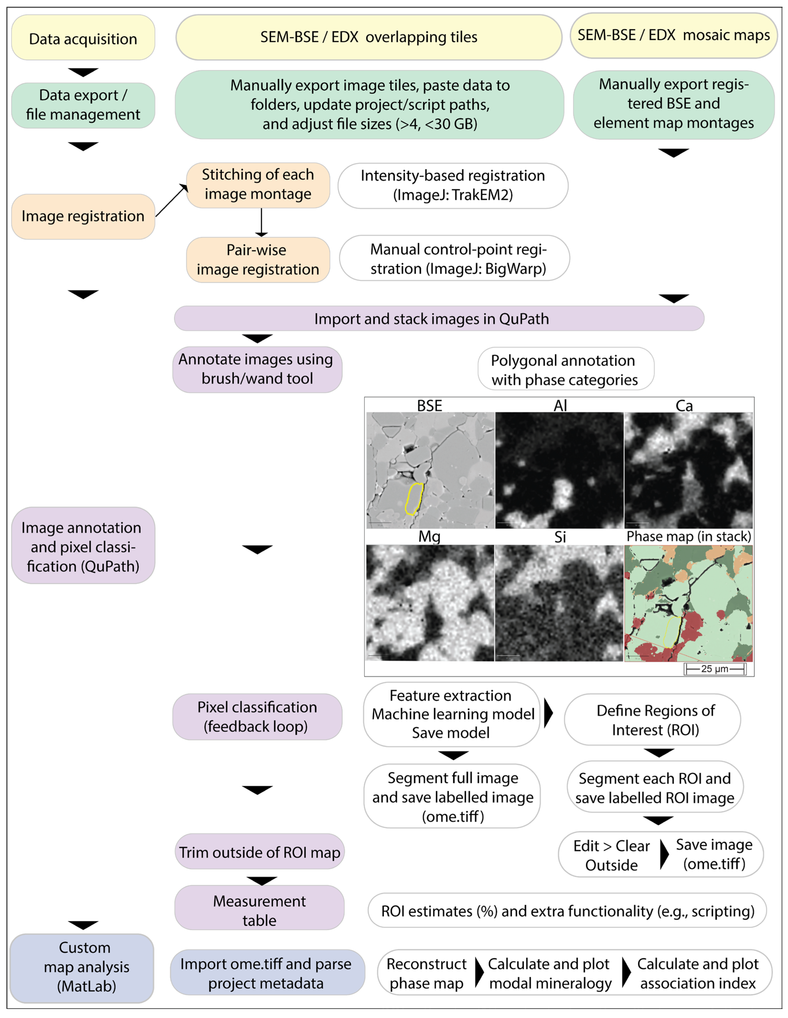
2. Materials and Methods

Three experimental charges were investigated for this study. They were selected from a much larger isobaric 5 GPa suite of mantle peridotite melting experiments. The wider research project aimed at investigating the disparate estimates for the 5 GPa lherzolite solidus [19], the question of whether orthopyroxene remains a stable phase at 50 °C either side of the solidus [1,19], and the disagreements regarding garnet versus clinopyroxene stability at advanced stages of melting between experiments and thermodynamic models [1,19,20,21,22]. Some of the current disagreements could potentially be related to undetected phases at very low abundance in experimental charges (i.e., low-degree melts and low abundance ortho- and clinopyroxene), which might be exposed by phase maps. The full results of these experiments will be reported elsewhere alongside the detailed experimental procedure. All experiments were conducted in a modified high-pressure, 500-ton end-loaded piston cylinder at the Australian National University (ANU). Further information on the piston cylinder apparatus and assembly materials used in this study were reported elsewhere [13,23].
We selected one equilibrated representative experiment each from below (UHP32, T = 1525 °C, 9 h) and above (UHP40, T = 1600 °C, 5 h) the solidus and one experiment that suffered a high thermal gradient (UHP21, nominal T = 1675 °C, 24 h), the bottom of the (overly tall) charge apparently failing to reach the target T. The thermal gradient in charge of UHP21 caused the establishment of melting reaction assemblages similar to those used in earlier studies to verify the saturation sequence [2,3]. Although this experiment has limited thermodynamic value, the exposed thermal gradient caused a stratified charge similar to those encountered in layered reaction experiments [6,7]. In all cases, due to the simple ultramafic system composition (GKR-001, Table 1), only very few phases were expected: olivine, orthopyroxene, garnet, clinopyroxene, melt, and possibly Cr-rich spinel. Observed phase relations were compared to those thermodynamically modeled with MAGEMin [24] based on the igneous dataset [20]. For EMPA analysis and imaging with SEM-BSE, the charges were prepared as follows: after the run, the recovered sample was mounted into epoxy and polished in water using 800- and 1000-grit sandpaper to expose the charge. After exposing a small section of the charge, polishing continued with 1200- and 2500-grit sandpaper to avoid sample loss and excessive mineral plucking during polishing. The final polishing stage was performed with diamond pastes (6, 3, 1, and 0.25 µm). Before carbon-coating the samples, the quality of the polish was carefully assessed using a reflected light microscope.
The composition of the solid phases is listed in Table 1 and was analyzed with standard EMPA protocol at the ANU (field emission gun (FEG)-equipped JEOL 8530F Plus (JEOL Ltd., Tokyo, Japan)). The EMPA was operated with an acceleration voltage of 15 kV, a beam current of 20 nA, and a nominal beam diameter of 1 µm in spot mode. The counting time for each element during the analysis was 20 s on the peak and 10 s on the background. For this study, the sole purpose of the chemical compositions was to calculate modal abundance via mass balance (Table 1). Petrological implications will be discussed with the full suite of experiments. The samples were also investigated by SEM-BSE and -EDS at QUT’s CARF laboratory on a Tescan MIRA-3 FEG SEM (Tescan, Brno, Czech Republic) [17] equipped with three EDS detectors, configured as a TIMA (Tescan Integrated Mineral Analyzer). After experimentation, the preferred setting for this project’s routine phase mapping imagery was as follows. For BSE (with Image Snapper), the acceleration voltage was 15 kV, at a beam intensity of 12.0, and with BSE scan setting S7 (100 µs/pixel). For EDS mapping, the acceleration voltage was 25 kV at a beam intensity of 19.9 and an X-ray count of 4000. For the small experimental charges (typically ca. 1.2 × ca. 0.6 mm), the BSE acquisition took 40–90 min, and the EDS maps 30–80 min. A series of exploratory scans were conducted to evaluate the influence of BSE scan speeds, EDS acquisition modes, and EDS count rates on phase map quality.
Sample UHP32 was additionally analyzed on a Hitachi SU7000 field emission SEM (Hitachi, Ltd., Tokyo, Japan) equipped with the Bruker AMICS automated mineralogy system at UQ Natural Resources Innovation Characterisation Hub (NRICH), again exploring different combinations of BSE scan speeds and EDS acquisition modes for optimal phase maps on experimental charges.
One main aim of this project was to devise and deploy an instrument-agnostic, offline, open-source software method for user-informed pixel-classified phase mapping optimized for fine-grained samples. The approach involves several consecutive steps that can be learned by a non-expert within a few hours. They are schematically illustrated in Figure 1. The process starts with the acquisition of BSE and EDS element maps. This is easiest as combined BSE and EDS images are montaged by the SEM software. Exported manually as individual BSE and element maps, they can move directly to image annotation and classification (Figure 1) because they are spatially registered.
Due to the occurrence of small x-y tile offsets in SEM-generated image montages that can create artifacts in very fine-grained charges, we opted to acquire the BSE imagery with 25% frame overlap in the Tescan MIRA3 software version 4.2.37.0 with the add-on Image Snapper at a slow scan setting S7 (100 µs/pixel). Original BSE tiles are exported individually. This type of BSE acquisition and export is offered on most modern SEMs. On the SEMs available for this project, it was not possible to obtain unstitched, overlapping EDS tiles corresponding to the BSE frames. Therefore, the EDS data were acquired separately as a TIMA version 2.11.1 experiment using the dot-mapping EDS approach (accelerating voltage 25 kV, pixel spacing 0.5 µm, dot spacing 1.5 µm, and field width 100 µm). Within the completed TIMA project, we exported individual X-ray intensity maps. Considering the chemistry of the phases, four element X-ray K-line maps were found sufficient for phase recognition (Al for garnet, Ca for clinopyroxene, and Mg and Si to distinguish between olivine and orthopyroxene).
Unless full montage images are exported, the next step is image registration. We first stitch the high-quality BSE tiles with the ImageJ2 software version 1.54c TrakEM2 plugin using globally optimized intensity-based registration [25]. This achieves a very good alignment, and the resulting high-quality BSE montage is then used as a fixed image for registration of the element X-ray K-line maps with control-point manual registration following a non-rigid transformation in BigWarp [26], a plugin extension of ImageJ2 [27]. For SEMs that permit the acquisition and export of concurrent, same-resolution BSE and EDS tiles with overlap areas, the registration of the BSE frames could be applied to the individual EDS element maps, obviating further co-registration.
Regardless, the co-registered montages (one BSE and 4 element X-ray layers) are now moved into the open-source software QuPath [28] version 0.4.2 for pixel classification. Import is performed as single-channel images into a new project, followed by building a stack. Using the ‘Interactive image combiner Warpy’ extension [29], a virtual ‘overlay’ of the imported images is generated, allowing users to simultaneously use all desired layers. On the multi-view canvas (Figure 1), the user can view and navigate all desired images. The brush and wand tools are deployed to annotate 12–15 polygons per phase category on the image stack. The interactive combined viewer is helpful in identifying the phase on the crisp BSE image with reference to the element maps. For example, in Figure 1, garnet is the BSE bright phase with high Al, intermediate Ca, and low Mg and Si intensities. Olivine and orthopyroxene, of indistinguishable BSE greyscale but present with recognizable grain contours on BSE, were distinguished with the Si and Mg intensity maps. Care is required to place the annotation polygon (yellow in Figure 1) on the stacked BSE image covering some of the grain interior and a grain edge, avoiding annotating the grain boundary itself.
With phase categories annotated, the pixel classifier tool can be deployed within QuPath. This yields the best results when looping at least twice through settings of ‘feature extraction’ and ‘random trees’ models. When the trained classifier yields realistic results, it is saved and deployed at ‘very high’ resolution (1 segmented pixel = 2 × 2 original pixels) for the final semantic segmentation maps. Pixel classification can be performed on the entire image or on smaller regions of interest (ROI). For statistical analysis of ROIs, the phase map is sent to ImageJ to clear the outside (pixels representing adjacent ROIs, epoxy, graphite, etc.) and saved. The QuPath toolbar option ‘Show measurement table’ displays object measurements from the semantic segmentation maps, including the pixel proportions, which can be converted to modal abundance.
Additional phase map analysis can be performed in MatLab version 24.2.0.274171 (R2024b) Update 1. For this, the ome.tiff files of the entire segmented images or trimmed segmented ROIs are opened in MatLab and turned into phase maps with options to determine modal mineralogy [18], multiresolution association matrices [30], and adjacency (or accessibility) maps [31]. The script and all QuPath projects, intermediate files, and maps are provided in the code (https://github.com/marcoaaz/Acevedo-Kamber/ accessed on 28 March 2025) and data (https://zenodo.org/records/14822997 accessed on 10 February 2025) repositories.

3. Results

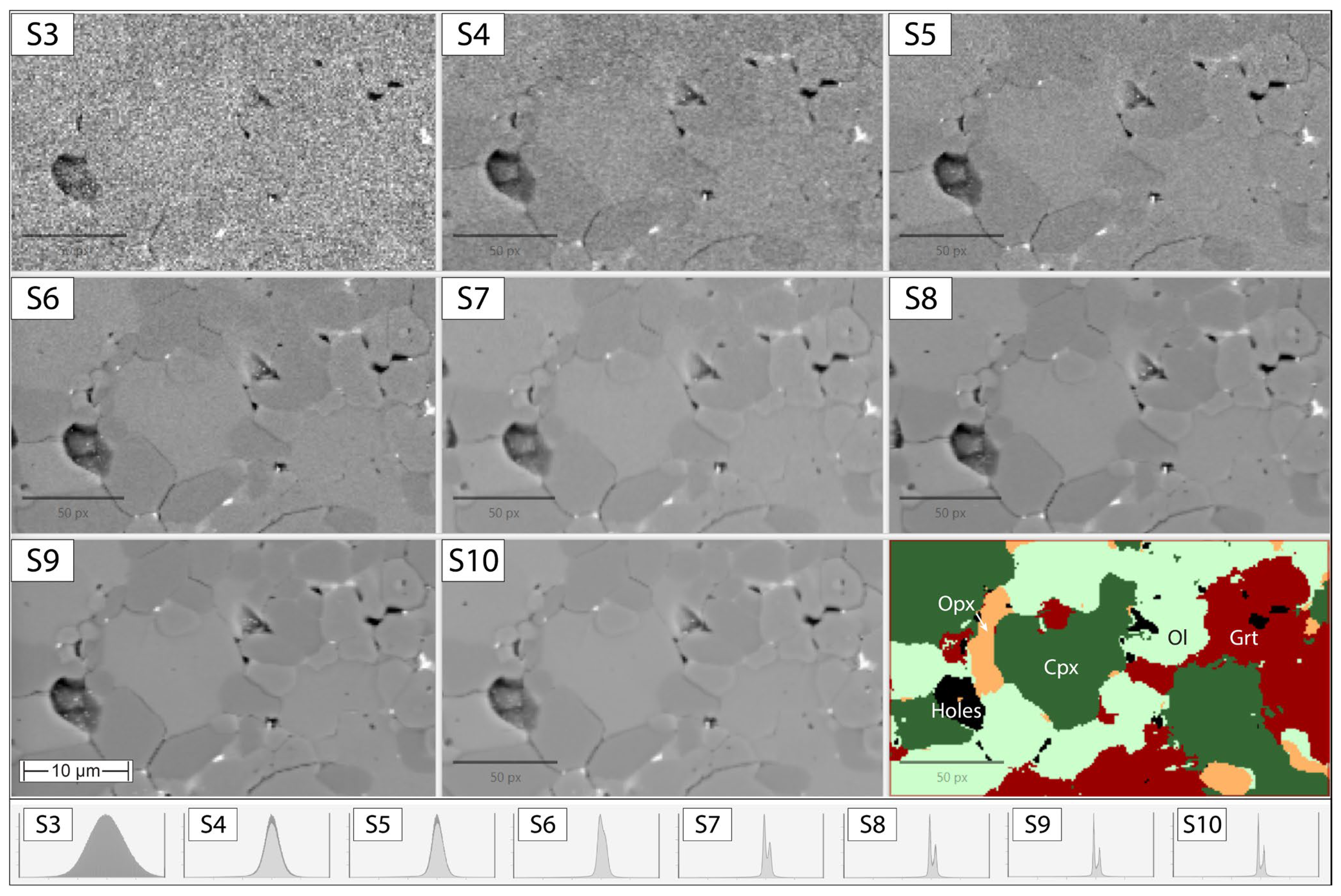
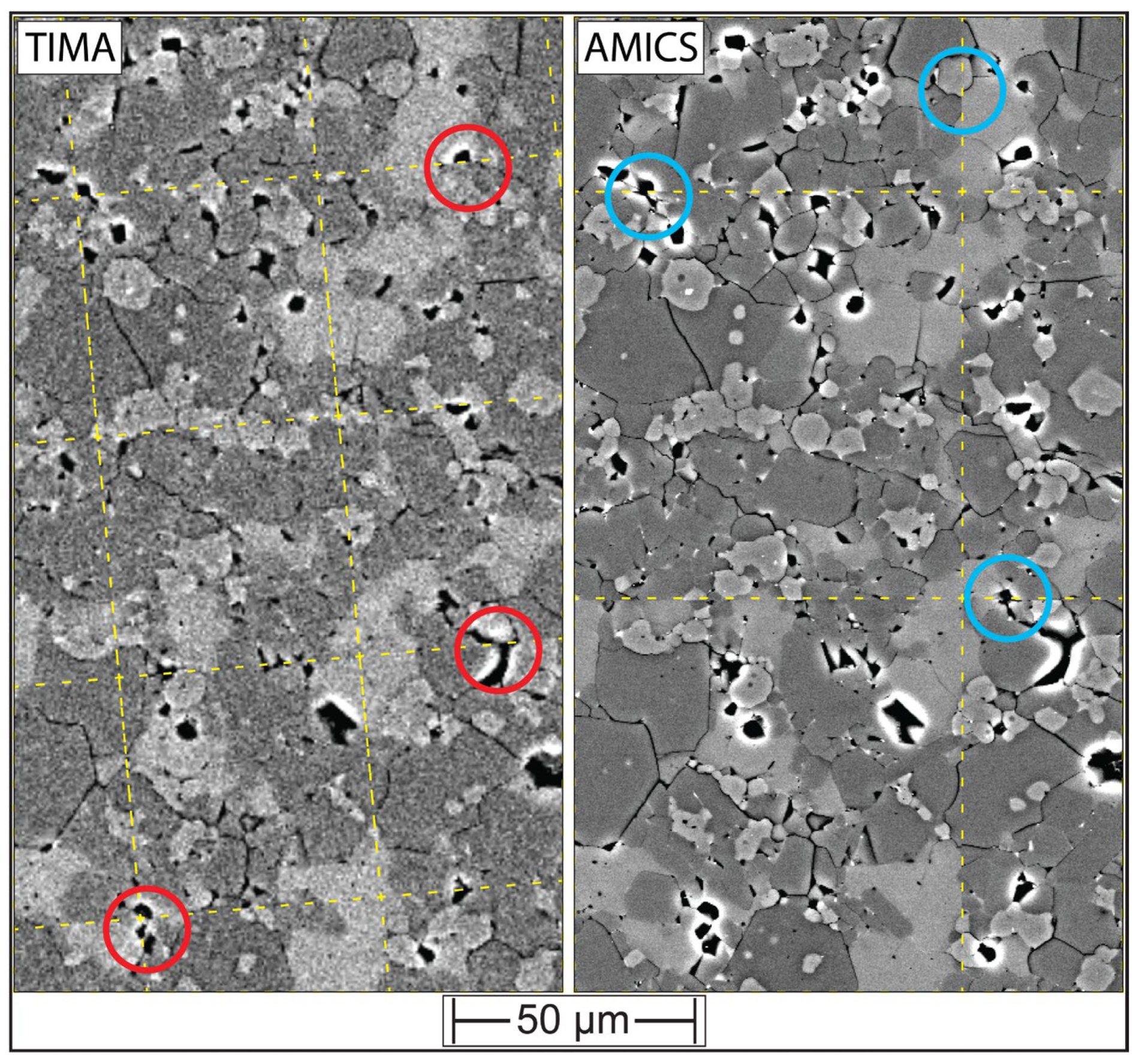
3.1. Evaluating BSE Scan Speeds and EDS Acquisition Settings

For commercial high-throughput or large-area applications of automated mineralogy, the SEM acquires a grid of adjacent frames with user-defined overlap. For each frame, the SEM first acquires a BSE image, which is then pre-segmented into areas of similar greyscale (‘segments’). Algorithms then find representative points within these polygons for EDS acquisition—typically called EDS ‘dot’ maps. After the acquisition of all the frames, their nominal stage x-y positions are used to construct the mosaic. Different options exist to merge grains of equal compositions along adjacent frames into phases. This is a significantly more economical approach for covering large area phase maps than a brute force high-spatial resolution grid EDS analysis (variably called ‘HR’, (HR), or ‘grid’ mapping, among others), but it relies on stable probe current delivered by the FEG [17]. Regardless, irrespective of the FEG-SEM instrument and proprietary phase mapping software used in this study (Tescan/TIMA and Hitachi/Bruker AMICS), we found stitching errors in the BSE montages of at least some of the experimental charges. Mostly, they were small x-y offsets, but in some cases, they led to a repetition of features in the phase maps. The stitching errors reflect the rapid way in which the proprietary software generates BSE montages from nominal frame positions without intensity- and feature-based registration and without operator input. For academic research on high-value targets, however, the time and effort involved in producing the best possible BSE montages is trivial.
For this reason, we obtained grids of unstitched BSE frames on the Tescan TIMA MIRA3 instrument with wide (25%) areal overlaps that were individually read, accurately montaged, and registered. To find the fastest BSE scanning rate on this SEM still yielding acceptable results for phase mapping of our charges, we performed a series of tests on a small area of the finest-grained, sub-solidus charge UHP32. These experiments encompass unreasonably fast to excessively slow scanning rates, and results are shown in Figure 2.
Qualitative visual inspection suggests that scan speed settings S3 to S5 are too fast, producing noisy BSE images with poorly resolved grain boundaries. At the slow scan speed end, settings S9 and S10 offer a limited return on time investment over S8. For example, area scans performed in S9 take 2.9 times longer than in S8, and S10 scans take 9.1 times longer than in S8. Realistic scan speed rates were therefore judged to be S6 to S8. To more thoroughly evaluate the effects of scan speed setting on grain boundary identification and greyscale level differentiation, we extracted greyscale intensity line profiles across sample UHP32. Figure 3 compares those obtained with BSE scan speed settings S6 through to S10.
The comparison shows that noise in scan speed setting S6 still obscures phase boundary definition but that scan speed settings S7 and S8 accurately locate phase boundaries. These two settings were, therefore, investigated further. Of note is that even with the slowest scan speed settings, S9 and S10 (lowermost profiles in Figure 3), the overall BSE intensity of orthopyroxene is not distinguishable from that of olivine. This peculiarity of the charges studied here contributed to the dearth of BSE contrast. For quantitative evaluation of the most time-effective accurate acquisition settings, individual phase maps were constructed with a permutation of BSE and EDS settings. A subset of the resulting phase maps is shown in Figure 4.
Two separate ground truth phase maps were generated. The first used a routine Tescan TIMA phase map acquisition setting, which combines fast BSE scanning (S4) with slow, high-spatial-resolution EDS mapping (pixel spacing 0.5 µm). Despite the substantial effort in selecting different combinations of element maps and phase map settings, it proved difficult to (i) avoid generating artificial phases along grain boundaries (mixed pixels = ‘mixels’), (ii) define less jagged (binary) grain boundaries, and (iii) avoid excessive attribution of pixels to ‘holes’. The default spectral library search incorrectly attributed all olivine and orthopyroxene pixels to the ‘olivine’ class, while clinopyroxene pixels were split into ‘diopside’ and less abundant ‘actinolite’. Therefore, a custom library was built for the phases shown in Figure 4, which required testing and adding compositional rules and the ‘clinopyroxene mixels’ class.
The second ground truth map was generated with the open-source software workflow combining the best BSE image with the HR EDS elemental maps (Al, Ca, Si, and Mg). This resulted in a crisp phase map, with realistic appearing grain boundaries, few holes, and a lack of ‘mixels’. It also managed to discern many olivine/olivine grain boundaries due to their fine surface irregularities being classified as holes. Additional phase maps were then generated with the open-source software workflow for a permutation of BSE scan setting imagery (S7 to S9) and HR and dot-mapping EDS element maps. Figure 4c,d compares the BSE S7 scan setting maps combined with the two EDS element maps. The visual comparison shows that they both show crisp grain boundaries (derived from the common BSE image). Finally, despite the much lower spatial resolution of the dot-based elemental maps, the resulting phase map (Figure 4d) appears visually very similar to that obtained with the higher-quality HR EDS map (Figure 4c).
To test the equivalence of the three phase maps with homologous pixel locations (Figure 4b–d), we calculated normalized confusion matrices (Figure 5), in which the highest-quality phase map (Figure 4b) was used as the true class, and the higher-speed phase maps were treated as the predicted class. This shows that the scan speed S7-HR phase map predicts the four minerals with an accuracy ranging from 95.6 to 97.5%. The quality of prediction follows the order of modal abundance. Holes were predicted with 83.3% accuracy. The S7-dot phase map also achieves very high accuracy prediction for the four main minerals, ranging from 85.8 to 93.7%, again in order of increasing modal abundance. Holes were detected with 74.3% accuracy. The inferior accuracy of the S7-dot phase map is very likely due to the much sparser density of EDS data and not due to the process of phase map construction, which used the same annotations for all three phase maps. Due to the much inferior BSE image underlying the TIMA phase map (Figure 4a) and the non-homologous pixel locations and sizes, no equivalence test was conducted.
We further evaluated the acquisition settings with a comparison of modal abundances (wt%) of the four rock-forming minerals. They were calculated from pixel numbers (Figure 1) on the phase maps and theoretical densities (olivine = 3.310; orthopyroxene = 3.338; clinopyroxene = 3.175; garnet = 3.600) for statistical comparison (Figure 6). Binary plots of BSE S7 and S8 with HR EDS mapping modal abundances are compared to the ground truth modal abundance from BSE S10 with HR EDS mapping. This showed very good proportionality with both comparisons (Figure 6a) on the small representative area on sample UHP32 (Figure 4) with no statistical difference between the S8 and S7 BSE scan speeds. Binary plots of BSE S7 with HR and dot EDS mapping were next compared to BSE S10 with HR EDS. Again, there is minimal statistical difference in the quality of the regression, suggesting that the somewhat lower pixel equivalence accuracy of the EDS dot mapping (Figure 5) does not materially skew the modal abundance estimate.

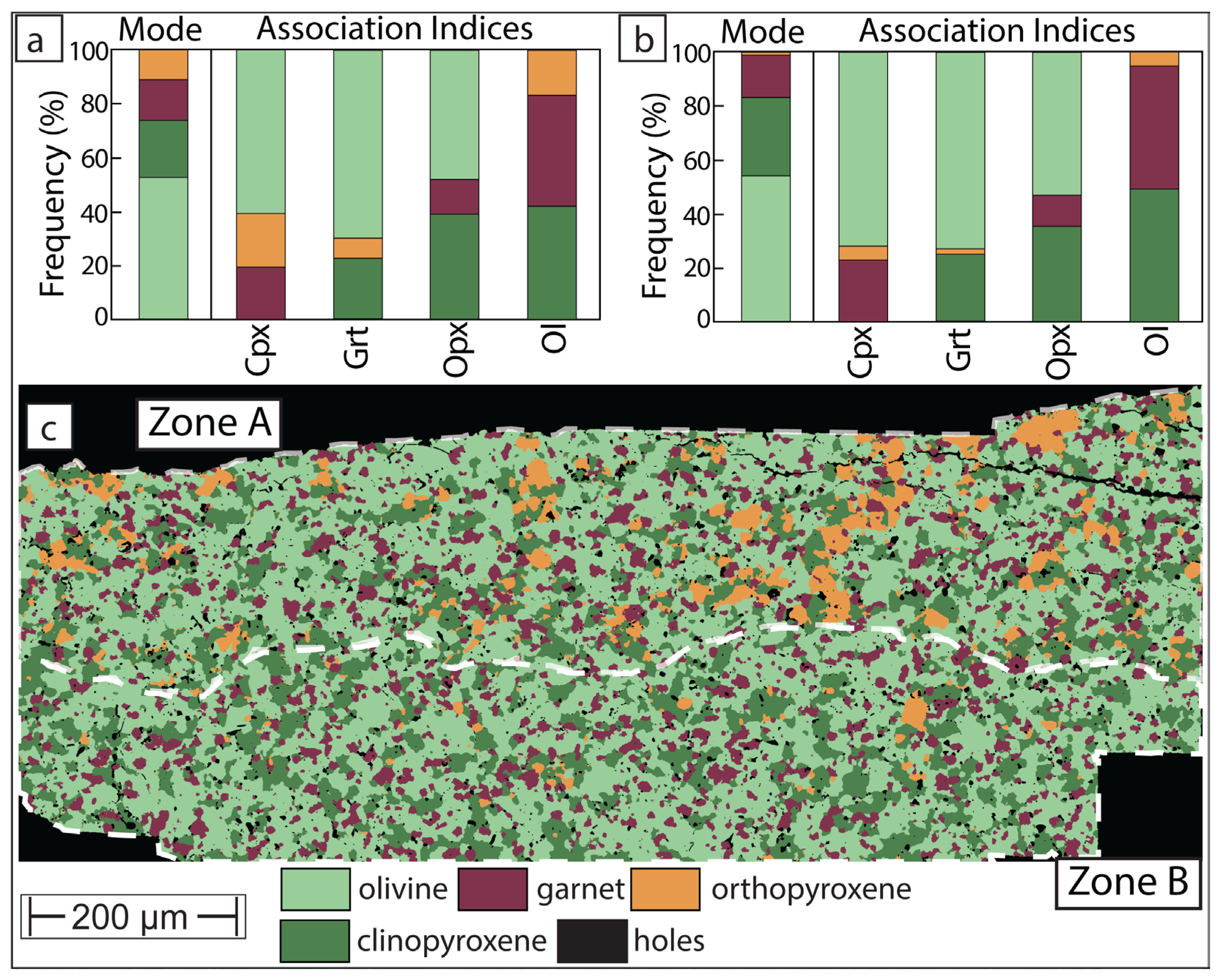
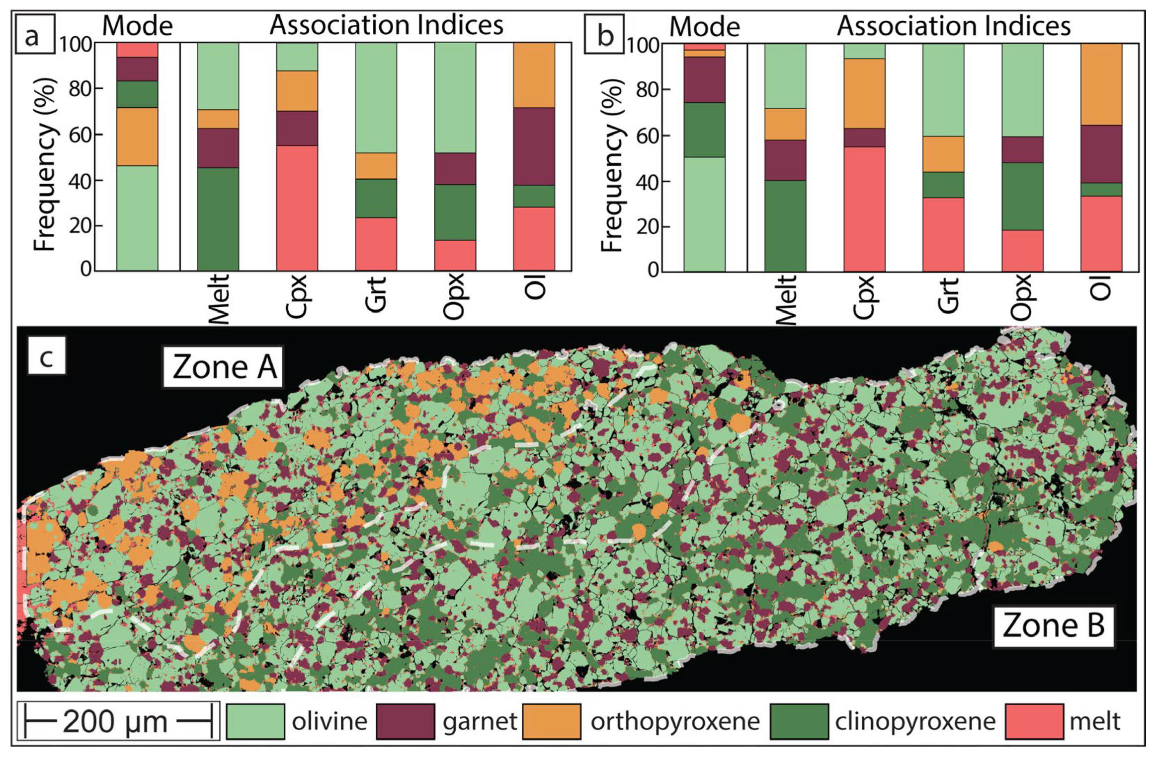
3.2. Phase Maps and Modal Mineralogy for Thermally Equilibrated Experiments

The full phase map for sub-solidus sample UHP32 (Figure 7) made with open-source software demonstrates a granular texture and a mode dominated by olivine and clinopyroxene. The frequency of pixels was used to determine the modes of the arbitrarily defined upper ‘Zone A’ and lower ‘Zone B’ (ROIs), the former with higher orthopyroxene abundance. The modes of both zones are displayed on the left-hand side in panels (a) and (b) of Figure 7. The comparison demonstrates that modally more abundant orthopyroxene in ‘Zone A’ is largely present at the expense of the compositionally similar clinopyroxene (Table 1). We note that the presence of orthopyroxene could be overlooked when inspecting ‘Zone B’ under real-time BSE on an EMPA, recalling that it has an indistinguishable BSE greyscale from olivine (Figure 3).
In the equilibrated melt-present experiment UHP40, the open-source software-generated phase map (Figure 8) again reveals some phase differentiation, with the upper layer (‘Zone A’) richer in orthopyroxene and melt and poorer in clinopyroxene and the lower, melt-poor layer (‘Zone B’) more similar in mode to the subsolidus sample (Figure 7). Like in sample UHP32, the presence of orthopyroxene is largely at the expense of clinopyroxene and, to a lesser extent, garnet.
Figure 7. Modes, phase associations, and phase map of sample UHP32. (a,b) show mode and mutual phase associations in ‘Zone A’ and ‘Zone B’ (defined as separate ROIs), respectively, of the phase map (c).
Minerals 15 00355 g007
Figure 8. Modes, phase associations, and phase map of sample UHP40. (a,b) show mode and mutual phase associations in ‘Zone A’ and ‘Zone B’, respectively, of the phase map (c).
Minerals 15 00355 g008

3.3. Phase Map for Experiment Which Did Not Experience Thermal Equilibrium

Sample UHP21 was from the early exploratory experiments of the project, in which much thicker (taller) charges were trialed (Figure 9). The target T, 1675 °C, was only reached at the top of the charge, while the bottom remained at a significantly lower T, similar to UHP40 (1600 °C). The resulting strong thermal gradient accidentally produced a reaction experiment, as often encountered in the pioneering high PT melting experiments [2,3], which were prone to thermal gradients. This is typically visualized in BSE with strong contrast in melt distribution and a pronounced preferred spatial distribution of phases. Examples of these can be found in Figure 1 of [2] and Figures 7, 9, and 10 of [3]. Although high thermal gradients are undesirable and petrologists repeat such experiments until thermal gradients are avoided, the distribution of phases across the thermal gradient is still interesting in terms of the relative stability of phases, i.e., the order of phase saturation [2,3]. It was anticipated that phase maps would more clearly demonstrate the spatial distribution across the thermal gradient than BSE imagery alone.
On the phase map produced with the open-source software method (Figure 9), the charge can be separated into two zones. The cooler temperature ‘Zone B’ is composed predominantly of olivine, clinopyroxene, and garnet with very little melt (2.3 wt%) and even less orthopyroxene. By contrast, the upper ‘Zone A’, which occupies the bulk of the charge, is mostly composed of olivine, orthopyroxene, and melt (14 wt%). In the higher temperature (nominally 1675 °C) ‘Zone A’, rare garnet (1 wt%) only exists as small inclusions in much larger olivine grains, and clinopyroxene (0.9 wt%) is largely confined to inclusions within olivine in proximity to ‘Zone B’. Some clinopyroxene also exists along orthopyroxene/melt grain boundaries, where it likely formed as a quench product from the melt (as also found in the much higher T experiments of [3]).
This phase distribution suggests that the charge formed across a temperature window of a major melt-forming reaction. This predominantly consumed clinopyroxene and garnet and produced peritectic orthopyroxene. The stoichiometry of this reaction at 5 GPa in lherzolite composition KR4003 was thermodynamically modeled [32] as follows:
0.31 olivine + 1.7 clinopyroxene + 0.19 garnet = 1 melt + 1.2 orthopyroxene,
This appears in good qualitative agreement with the distribution of phases in the map of sample UHP21 and illustrates that ‘failed’ experiments exposing thermal gradients may contain value in terms of verifying reactions that are normally calculated based on mass balance [33] rather than microstructural observations.

4. Discussion

The discussion is structured into two sections, the first delving deeper into the utility of phase maps to investigate high PT experimental charges and the second focusing on instrument settings for generating phase maps suitable for experimental charges.

4.1. Insights from Phase Maps of High PT Charges

Beginning with the subsolidus sample UHP32, the modal abundance estimated from its phase map (Figure 7) compares very well with that obtained from mass balance (Table 1). The two estimates correspond closely (Figure 6c) and yield a regression slope of 0.9972 with an r2 of 0.9987. This demonstrates that although the phase map is obtained from a 2-dimensional slice through the charge, it is a valid representation of the overall system and of the phase chemistries, which inform the modal mineralogy obtained via mass balance. More importantly, the very good agreement between the methods is a strong test of the accuracy of the starting composition. The production of synthetic rock system compositions can involve many steps that include multiple weighing and handling of powders with associated uncertainties. The tight agreement between the two independent methods of estimating modal mineralogy confirms the accuracy of the starting composition and the EMPA phase chemistry. Furthermore, the agreement in modal mineralogy also confirms the isochemical nature of the experiment, at least for the major rock-forming oxides. Namely, it is not uncommon for high T experimental charges to lose redox-sensitive species (e.g., Fe) to the assembly, resulting in an undesired unintentional change in the system chemistry (see, e.g., [34]). In subsolidus charges, independent modal abundance estimate agreement warrants against loss or gain of major system components. However, in charges containing melt that has likely migrated, the 2-dimensional phase map is unlikely to be quantitatively representative.
A further strength of phase maps is that they can be used to quantify mineral associations. This is an active research field in mineral processing, liberation, and exploration [35], whereas, in metamorphic and igneous petrology, mineral association matrices have traditionally been used to test local equilibrium (e.g., [36]). The spatial information contained in computed phase maps can be used to calculate quantitative information about mutual mineral (or phase) contacts. For sub-solidus sample UHP32, the mineral association matrix (Figure 7) confirms that all four rock-forming minerals are in mutual contact. In both the upper and lower ‘Zones A’ and ‘B’, pixels of the most abundant mineral, olivine, are in contact with all other minerals with no clear preferences. By contrast, ortho- and clinopyroxene are in preferential contact, sharing more pixel boundaries than could be expected from modal abundance. Because the mineral association index is sensitive to the accurate classification of pixels at the periphery of grains, we made a comparison between phase maps obtained with the various BSE and EDS settings of the small area map of sample UHP32, shown in Figure 4. This revealed very similar mutual contact relationships and confirmed the strong association of the two pyroxenes (Figure 10).
The surprisingly uneven distribution of ortho- and clinopyroxene across ‘Zone A’ and ‘B’ could have two mutually inclusive reasons. First, very minor heterogeneity in the starting mixture (e.g., Ca) could cause significant changes in pyroxene modes, considering the overall similarity in the chemistry of both pyroxenes. Secondly, at the PT conditions of these experiments, ortho- and clinopyroxene have near-identical entropies and very similar enthalpies [37], meaning that the minimum energy of the system is insensitive to the ratio of the pyroxenes.
Turning next to sample UHP40, we note that the agreement between mass balance and phase map-derived modal abundance is inferior (Table 1 and Figure 6c). The modal abundance estimates agree well for the two most abundant phases (olivine and clinopyroxene) but diverge for garnet, orthopyroxene, and melt. This is most likely explained by the unrepresentativeness of the 2-dimensional exposure through the charge. According to mass balance, this experiment produced 7.7 wt% melt, yet the phase map only identified 3.4 wt%. This is almost certainly due to the heterogeneous distribution of melt, which tends to coalesce towards the edges of charges, in this case underrepresented in the exposed surface of the charge. Instead, the phase map overestimates orthopyroxene and garnet. The effort to produce a quality phase map (ca. 3 h SEM instrument time and ca. 3 h work for segmentation) might not be justified for such an experiment. However, phase maps with minor stitching errors can be acquired more rapidly (ca. 30–45 min per charge) at reduced SEM resolution, typically in unsupervised overnight runs of several samples. The processing time can also be reduced to ca. 60–90 min if the SEM-generated mosaic is used (Figure 1, right-hand side). The resulting fast phase maps still offer sufficient clarity for phase targeting on the EMPA. With respect to charge UHP40, the power of the phase map (Figure 8) is illustrated with two examples. First, within ‘Zone B’, melt is in very low abundance, but the phase map can guide the analyst to the largest ‘films’ or pools of it ahead of operating the EMPA. There is considerable disagreement in the existing experimental literature about the 5 GPa solidus T (e.g., [19]), and thermodynamic models tend to position the lherzolite solidus at higher T than the most modern experiments, particularly at P > 3 GPa [21,38]. Second, the phase map illustrates that in ‘Zone B’, there are only very few grains of orthopyroxene (3.1 wt% modal abundance) while the BSE greyscale indistinguishable olivine is in much higher modal abundance (49.2 wt%). It is plausible that such a low proportion of orthopyroxene could have been missed based on BSE inspection alone. Although the orthopyroxene distribution close to the lherzolite solidus at 5 GPa may seem an academic question, its potential persistence across the solidus does have petrological implications. In the lherzolite bulk composition KR4003, the 4–6 GPa experiments of [1] were reported to be orthopyroxene-free over a ca. 50 °C T window across the solidus. Technically, such peridotites would classify as wehrlites rather than lherzolites, and the participation of pyroxenes in partial melting would have significant effects on the trace element partitioning into the melts. By contrast, 5 GPa experiments on KR4003 by [19] reported orthopyroxene across the solidus, similar to the charges shown in Figure 7 and Figure 8. At least some of these discrepancies could have arisen from unidentified low abundance orthopyroxene of indistinguishable BSE greyscale as olivine. Retrospective phase mapping of historic high PT charges has the potential to test this hypothesis.
Finally, the phase map of UHP40 demonstrates gradation in mineralogy, principally from a clinopyroxene-rich and very orthopyroxene-poor ‘Zone B’ at the bottom of the charge to an orthopyroxene-rich and clinopyroxene-poorer top left ‘Zone A’. This change in mineralogy is suggestive of a melt-producing reaction (1), incongruently consuming clinopyroxene and generating peritectic orthopyroxene. This is supported by the phase association matrix. In both ‘Zones A’ and ‘B’ (Figure 8), clinopyroxene is dominantly in contact with melt, closely followed by garnet. The persistence of the melt + clinopyroxene + garnet spatial association thus suggests that melt migration was not excessive in this experiment. Namely, had melt mostly percolated towards the top of the charge away from the original site of melting, the preferential spatial association would not be expected.
Thermodynamic modeling of the GKR-001 system shows that at 5 GPa, 16.6 wt% melt forms over a temperature window of only 16 °C. As can be seen from the corresponding modal abundance plot (Figure 11), over this melt generation interval, modeled clinopyroxene abundance in the solid drops from 32.2 wt% to 0 wt%, while orthopyroxene abundance increases from 0.5 wt% to 16.6 wt%. Modeling also predicts a more modest rate of garnet consumption compared to clinopyroxene, compatible with the phase distribution of ‘Zone A’ in Figure 8. Thus, although a small thermal gradient existed across the UHP40 charge, this was less than 16 °C, as melt is already present at the bottom of ‘Zone B’ while some clinopyroxene persists at the top of ‘Zone A’. The rapid change in mineralogy and melt productivity over a very narrow temperature range seen in charge UHP40 illustrates the difficulty of experimentally determining the exact solidus of lherzolitic to mildly refractory peridotite at high P [19].
The final point of discussion concerns experiment UHP21, displaying a ca. 75 °C thermal gradient, which caused it to unintentionally expose at least one major melting reaction. Disequilibrium is generally avoided in petrological experiments; however, with the wider realization of open-system behavior in magmatic processes, there is a growing need for reaction experiments. These are typically achieved by juxtaposition of two or more chemical compositions in layered reaction experiments. Reactions are observed at the interface between layers (e.g., [7]) but also via migration of melt from a more fertile lower layer through a more refractory upper layer (e.g., [6]). To date, such experiments have largely relied on BSE overview scans with manual phase annotations for documentation, yet phase maps and their analysis (e.g., association matrices) appear ideal instruments to more quantitatively study reactions. Thus, although UHP21 was neither layered nor a deliberate reaction experiment, its microstructure still lends itself to illustrating the utility of phase maps for studying reactions.
In this charge, the bottom ‘Zone B’ resided close to the solidus (Figure 9), with similar modal abundances as in ‘Zone B’ of the equilibrated experiment UHP40 (Figure 8). The bulk of the charge experienced substantially higher T, close to the target 1675 °C, with no clinopyroxene and hardly any garnet remaining. The spatial phase distribution across the thermal gradient implies the following relative stability: liquid -> olivine -> orthopyroxene -> garnet -> clinopyroxene. Compared to observations from similar lherzolite charges with thermal gradients at 6 GPa [2], this suggests a reversal of garnet and orthopyroxene in the stability order between 5 and 6 GPa. This is currently not accurately reproduced by thermodynamic models (e.g., [20,21,22]).
The paucity of non-included clinopyroxene in ‘Zone A’ suggests melting at 1675 °C proceeded beyond the clinopyroxene-out reaction (Figure 11) that involved all three remaining minerals. The stoichiometry of this type of reaction at 5 GPa in lherzolite composition KR4003 was thermodynamically modeled [32] as follows:
0.29 olivine + 0.47 orthopyroxene + 0.24 garnet = 1 melt
The distribution of garnet in ‘Zone A’ shows a preponderance as inclusions in olivine with no garnet in touch with the melt network in the top half of the charge. This suggests that reaction (2) ran to completion, and garnet was only accidentally preserved as non-touching olivine inclusions seen with ‘gi’ annotations on the UHP21 phase map (Figure 9). Their survival within olivine suggests that 1675 °C was insufficient for the garnet-out reaction [32]:
0.30 garnet + 0.70 olivine = 1 melt
In other instances, garnet coexists with touching melt as olivine inclusions (labeled ‘gmi’ in Figure 9). They are found across ‘Zone A’ of the charge, suggesting that they represent formerly touching orthopyroxene + garnet inclusions in olivine, where reaction (2) proceeded to orthopyroxene exhaustion. The intricacies of these inclusions and potential melting reactions have no petrological significance due to the poorly constrained T of the experiment. However, the preservation of microstructures, reaction textures, and local miniature chemical systems can only properly be appreciated on phase maps and would be very difficult to infer from BSE scans alone. When applied to deliberate reaction experiments from layered charges, phase mapping will be powerful in elucidating the consumption and precipitation of phases.

4.2. Working Towards Optimized Operating Procedures for High-Quality Phase Maps of Experimental Charges

For a wider uptake of phase mapping of experimental charges, it is desirable for proprietary automated mineralogy solutions (e.g., Tescan TIMA, Bruker AMICS, Oxford Instruments AZtecMineral, Thermo Scientific Maps, etc.) to generate suitable phase maps without the need for external image analysis. This study obtained phase maps with two commercial systems, both of which returned accurate modal abundance estimates but also contained some artifacts, most commonly small x-y translation errors on the stitched mosaics. In Figure 12, such SEM-BSE montage registration offsets are illustrated for TIMA (red circles on a fast acquisition BSE) and AMICS (cyan circles on a slow acquisition BSE). They are caused by stage drift and can be compounded by lens distortion and poor beam alignment (e.g., [37]).
The frame offsets are minor and would not impact most automated mineralogy projects. However, misaligned mosaic inputs can negatively affect the ability of computer-assisted segmentation and classification into objects [39] because mineral grains that extend across poorly registered frames have unnatural straight boundary segments, right angles, or jagged contacts with neighboring grains. The misalignments in the simple x-y translation mosaics can be fixed offline with external post-analysis image processing (e.g., [40]). However, this is only possible when the original overlapping frames are available (an example of a fixed AMICS montage is provided in the data repository). Regardless, when setting up a phase mapping project it is desirable to minimize stage travel and to find a good balance between the size of the field of view versus spatial resolution and distortion. This may require some preliminary experimentation on a given SEM-EDS.
With both systems used in this study, the common observation was that the best phase maps were generated by combining relatively slow BSE scan rates with the ‘dot-mapping’ EDS approach. While it might, at first, seem counterintuitive to dedicate more time to the BSE acquisition, the consistent finding was that a high-quality BSE scan results in better initial segmentation and definition of fewer polygons that needed to be investigated for EDS analysis. For example, on the Bruker AMICS system, the phase map shown in Figure 10 was obtained in 11 min and 46 s, combining 32 µs dwell BSE with dot EDS mapping. Using 16 and 8 µs BSE dwells with dot EDS mapping increased the acquisition times to 13 min and 7 s and 16 min and 27 s, respectively. This is because the faster BSE scans identified more watershed ‘segments’ (polygons) than necessary, thereby inflating the number of dot EDS analysis points. Furthermore, the faster dwell time BSE-based phase maps also showed more jagged and pixelated grain boundaries. On the Tescan TIMA, we found that 32 and 100 µs BSE dwell times resulted in quality BSE maps, while even longer dwell times offered no further advantage (Figure 2 and Figure 3). On AMICS, we also compared dot-mapping EDS with HR or matrix mapping at very close pixel spacing (0.5 µm) and found no advantage despite the substantially longer acquisition time (e.g., 122 min for a phase map the size shown in Figure 13). The equivalence comparison between HR and dot EDS mapping on the Tescan instrument (Figure 5) showed that HR acquisition may be warranted for experiments that produce very fine-grained charges or yield fine-grained trace phases. In summary, for the relatively small areas occupied by experimental charges, it is practical to obtain high-quality BSE imagery as the basis for rapid dot EDS mapping. The resulting phase maps also have practical applications beyond testing equilibrium, closed systems, or reactions. For example, phase maps can be imported into laser-ablation instruments and coordinated with their reflected light imagery for accurate trace element targeting that is otherwise very challenging. For SEMs not equipped with mineral liberation analysis software, the experience gained from this project suggests dedicating more acquisition time to BSE than EDS after suitable instrument-specific evaluation on small test mapping areas.
In terms of phase identification with commercial software, we found that on both systems used, it is desirable to build up a bespoke mineral library rather than relying on reference to the system-provided (large) mineral database. Because experimentalists generally have a good idea of the expected phases present in their charges, the comparison of EDS spectra with large reference databases is unnecessarily cumbersome. Furthermore, the reference libraries often contain multiple entries for solid/solution series (e.g., Mg- versus Fe/olivine) which can lead to unnecessary overcomplication when classifying pixels into phases. However, building a bespoke phase library does rely on the operator having a good understanding of EDS spectra and spectral interferences.
The user-driven open-source phase mapping software workflow proposed here can be applied to corresponding BSE and EDS element maps from SEM instruments that do not have dedicated phase mapping software. The software also has applications for petrographic thin sections. In most academic research projects, the investigator will have spent considerable time and effort inspecting the sample with a petrographic microscope before progressing to the SEM. Through optical microscopy, the investigator will thus have established the mineralogy of the rock forming phases as well as identified most of the accessory phases unless the sample is very fine-grained or mineralogically very complex. This knowledge is a pre-requisite for annotating and training the pixel classifier in our open-source workflow. The additional information from EDS spectra on rare or very finely grained accessory phases can then be used to identify the phases for which optical mineralogy did not yield conclusive answers. Thus, a user-driven approach is more likely to avoid erroneous misidentification of phases from a generic SEM-EDS spectral library. Such misattributions could, for example, arise from EDS spectral artifacts or from combining unrelated spectra of low-integrated signals from adjacent unrelated pixel groups.
One final difference between instrument software-generated phase maps and the user-annotated workflow presented here concerns boundaries between grains of the same phase. For such a comparison, we re-registered an instrument-generated phase map to correct for the small x-y offsets shown in Figure 13. This resulted in improved stitching (Figure 13a), but the classified mineral pixels yielded a phase map that looks ‘flatter’ than the microstructure of the experimental charge. When the same phase map was stacked with the original BSE layer and then annotated in QuPath (Figure 13b), the resulting phase proportions expectedly remained unchanged, but the microstructure appeared more realistic. Namely, the monolithic background of olivine in Figure 13a is broken up into subgrains, separated by narrow boundaries of pixels attributed to ‘holes’ (Figure 13b, white arrows). With a clearer appreciation of subgrains, it is also easier to identify included minerals versus interstitial grains (red arrows in Figure 13b). The improved representation of microstructure stems from a combination of factors. First, we used the BSE layer in the QuPath image stack to define the annotations. It contains much more structural detail than the EDS element maps that underpin the instrument-generated phase map. Second, we carefully applied the brush and wand tool to classify pixels to the exact edge of grains or subgrains (Figure 1). Third, we used classification trainers at high pixel resolution. Finally, as can be seen in the association matrix (Figure 10), holes are dominantly associated with olivine, suggesting plucking along grain boundaries.
Notwithstanding the utility of pixel-based classification for obtaining modal abundance and determining association matrices (Figure 7, Figure 8 and Figure 9), a true analysis of micro-structure requires grouping all pixels of a single grain into an object. This information yields additional insight into mutual contact relationships of actual mineral grains and sub-grains as well as melt films and pockets (where present). Namely, even though the microstructure of the pixel-classified phase map in Figure 13b looks realistic, it contains no actual information about which pixels belong to individual grains, for example, of olivine. Merging of pixels belonging to one object requires additional crystallographic information, typically obtained with electron back-scattered diffraction (EBSD) [41] or multi-angle cross-polarized light microscopy [42]. Only with such information is a deeper analysis of mineral and melt fabrics possible, for example, to establish crystal preferred orientation, topotaxic growth, or eutectic crystallization (e.g., [43]). Thus, additional data layers (e.g., EBSD) may further benefit the phase mapping of experimental charges.
Other additional data layers that could be integrated with phase maps are trace element maps obtained with high spatial resolution instruments. Due to the fine-grained nature of high PT experimental charges, it is difficult to obtain low-detection limit analysis for trace elements from conventional spot analysis, for example, with laser ablation. Phase maps are potentially also helpful for positioning the laser ablation analysis sites on experimental charges, which cannot be viewed in transmitted light. Full trace element maps on experiments have already been shown to yield improved trace element partitioning between melts and solids in high PT charges [44]. When combined with phase maps, all pixel locations of a phase can be pooled, and their collective trace element signal can be quantified to obtain lower detection limits (e.g., [45]), opening the prospect of better partition coefficients for trace elements that are in low abundance.

5. Summary

This study explored the utility of phase maps for the characterization of high PT experimental charges, with the following summarized findings:
  • Due to their small sizes, it is feasible to obtain high-quality BSE and EDS imagery for high PT experimental charges, requiring reasonable SEM instrument time (1 to 3 h). This effort is modest in relation to the production of the experiment and analysis of phase chemistry on the EMPA.
  • Phase maps of experimental charges give readers more tangible and complete evidence of phase equilibrium and phase relations than microphotographs of representative areas alone.
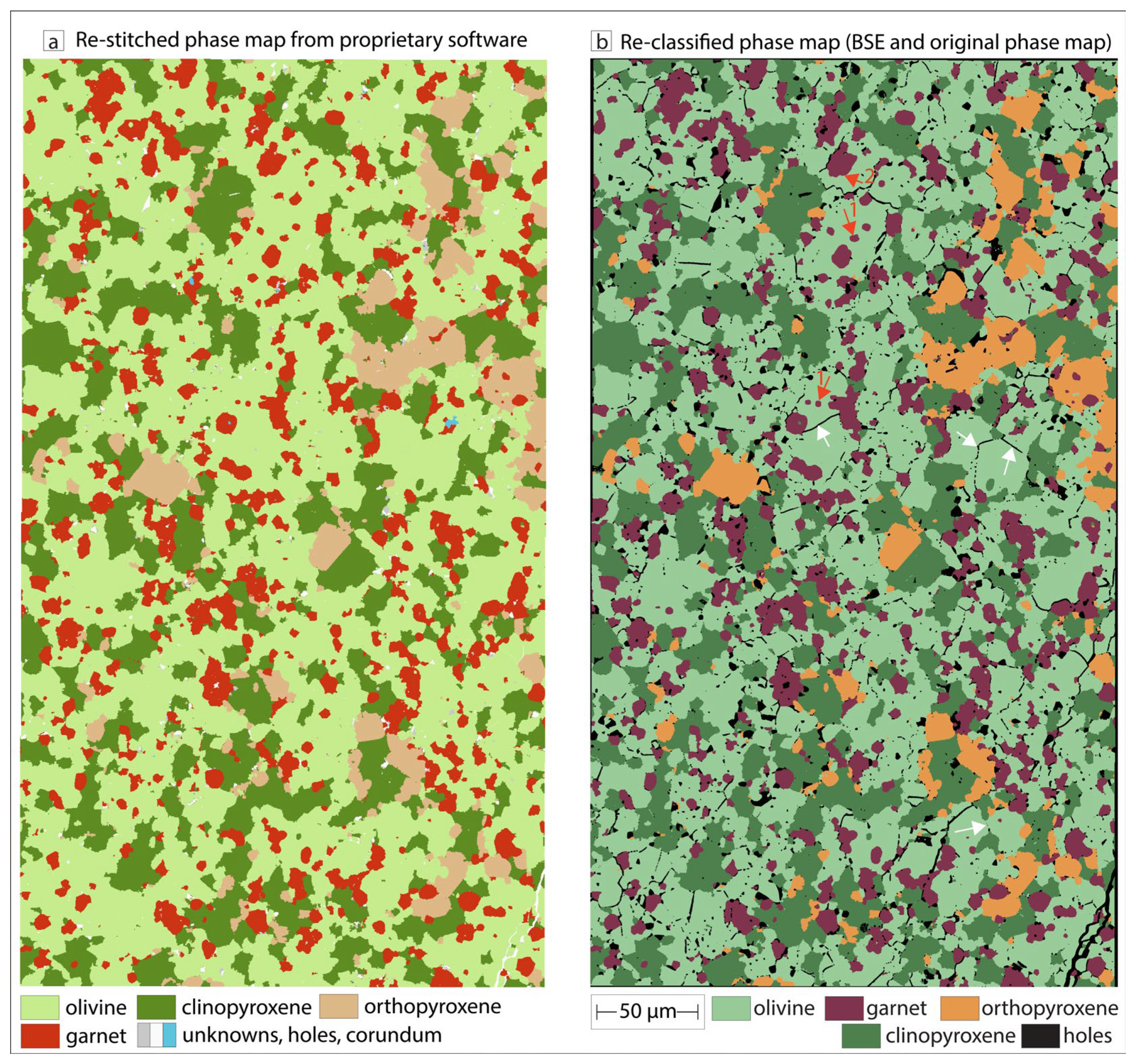
  • Phase maps generated with commercial automated mineralogy software are suitable to document phase relationships within charges, constrain modes, test for equilibrium, and identify EMPA analysis targets.
  • For charges with phases in low abundance or similar atomic number, open-source user-assisted phase mapping with high-resolution BSE images holds greater promise for obtaining accurate modal abundance estimates than those generated with current proprietary software.
  • In the studied sub-solidus charge, the system chemistry calculated from the phase map corresponded very well with the nominal chemistry and demonstrated a closed system.
  • Phase maps are particularly suitable for charges exposing reactions, for example, caused by chemical potential in layered experiments.
  • In charges with reactions, mutual pixel neighborhood relationships (quantified as association indices) can be used to verify the plausibility of mass balance-derived stoichiometries.
  • Phase maps have the potential to add retrospective additional value to historic experimental charges.
  • In the future, when combined with high spatial resolution trace element geochemical maps, phase maps have the potential to improve counting statistics for low abundance trace elements.

Author Contributions

Conceptualization, B.S.K. and M.A.A.Z.; methodology, M.L., M.N. and M.A.A.Z.; software, M.A.A.Z.; validation, M.L. and M.N.; formal analysis, all; investigation, R.F.R.; writing—original draft preparation, B.S.K., R.F.R. and M.A.A.Z.; writing—review and editing, all; visualization, M.A.A.Z., B.S.K. and R.F.R.; supervision, G.M.Y. and B.S.K.; project administration, B.S.K. and G.M.Y.; funding acquisition, B.S.K. and G.M.Y. All authors have read and agreed to the published version of the manuscript.

Funding

This research was funded by the Australian Research Council, grant number DP220100136 and AuScope Opportunity Fund 3.10505. R.F.R. received an international student Research Training Program PhD scholarship from the Australian Government.

Data Availability Statement

The full input images, intermediate files (images and metadata), and output phase maps are provided as the code (https://github.com/marcoaaz/Acevedo-Kamber/ accessed on 10 February 2025) and data (https://zenodo.org/records/14822997 accessed on 10 February 2025) repositories. The workflow to re-stitch AMICS software image tiles can be found as a commented script ‘imageJ_stack_matthew_v3.py’.

Acknowledgments

We thank two anonymous journal reviewers for very helpful suggestions for improvement. We acknowledge David Clark’s assistance in the high-pressure experimental petrology laboratories at ANU. EMPA analyses were supported by the Centre for Advanced Microscopy, an advanced imaging facility under Microscopy Australia, funded by the Australian National University and Australian State and Federal Governments. We thank Jeff Chen, Frank Brink, Corinne Frigo, and Eric Lochner for their assistance with quantitative WDS analyses of these experiments. We thank Eligiusz Gugula for technical input on phase mapping. NewSpec Pty Ltd., Hitachi High-Tech, Bruker, and The University of Queensland Centre for Microscopy and Microanalysis are thanked for access to Hitachi SU7000 FE-SEM with Bruker EDS detectors and AMICS software.

Conflicts of Interest

Matthew Ng was employed by the company NewSpec Pty Ltd., who had no role in the design of the study; in the collection, analyses, or interpretation of data; in the writing of the manuscript, and in the decision to publish the results. The other authors declare no conflicts of interest.

References

  1. Walter, M.J. Melting of garnet peridotite and the origin of komatiite and depleted lithosphere. J. Petrol. 1998, 39, 29–60. [Google Scholar]
  2. Canil, D. Orthopyroxene stability along the peridotite solidus and the origin of cratonic lithosphere beneath southern Africa. Earth Planet. Sci. Lett. 1992, 111, 83–95. [Google Scholar]
  3. Herzberg, C.; Gasparik, T.; Sawamoto, H. Origin of mantle peridotite: Constraints from melting experiments to 16.5 GPa. J. Geophys. Res. Solid Earth 1990, 95, 15779–15803. [Google Scholar] [CrossRef]
  4. Daczko, N.R.; Kamber, B.S.; Gardner, R.L.; Piazolo, S.; Cathey, H.E. Signatures of komatiite reactive melt flow through the Archaean Kaapvaal cratonic mantle. Contrib. Mineral. Petrol. 2025, 180, 5. [Google Scholar] [CrossRef]
  5. Lissenberg, C.J.; MacLeod, C.J. A reactive porous flow control on mid-ocean ridge magmatic evolution. J. Petrol. 2016, 57, 2195–2220. [Google Scholar]
  6. Yaxley, G.M.; Green, D.H. Reactions between eclogite and peridotite: Mantle refertilisation by subduction of oceanic crust. Schweiz. Mineral. Und Petrogr. Mitteilungen 1998, 78, 243–255. [Google Scholar]
  7. Mallik, A.; Dasgupta, R. Reaction between MORB-eclogite derived melts and fertile peridotite and generation of ocean island basalts. Earth Planet. Sci. Lett. 2012, 329, 97–108. [Google Scholar]
  8. Ezad, I.S.; Blanks, D.E.; Foley, S.F.; Holwell, D.A.; Bennett, J.; Fiorentini, M.L. Lithospheric hydrous pyroxenites control localisation and Ni endowment of magmatic sulfide deposits. Miner. Depos. 2024, 59, 227–236. [Google Scholar]
  9. Song, W.; Xu, C.; Veksler, I.V.; Kynicky, J. Experimental study of REE, Ba, Sr, Mo and W partitioning between carbonatitic melt and aqueous fluid with implications for rare metal mineralization. Contrib. Mineral. Petrol. 2016, 171, 1. [Google Scholar]
  10. London, D. The application of experimental petrology to the genesis and crystallization of granitic pegmatites. Can. Mineral. 1992, 30, 499–540. [Google Scholar]
  11. Brey, G.P.; Köhler, T. Geothermobarometry in four-phase lherzolites II. New thermobarometers, and practical assessment of existing thermobarometers. J. Petrol. 1990, 31, 1353–1378. [Google Scholar] [CrossRef]
  12. Nickel, K.G.; Green, D.H. Empirical geothermobarometry for garnet peridotites and implications for the nature of the lithosphere, kimberlites and diamonds. Earth Planet. Sci. Lett. 1985, 73, 158–170. [Google Scholar]
  13. Sudholz, Z.J.; Yaxley, G.M.; Jaques, A.L.; Brey, G.P. Experimental recalibration of the Cr-in-clinopyroxene geobarometer: Improved precision and reliability above 4.5 GPa. Contrib. Mineral. Petrol. 2021, 176, 11. [Google Scholar]
  14. Albarede, F.; Provost, A. Petrological and geochemical mass-balance equations: An algorithm for least-square fitting and general error analysis. Comput. Geosci. 1977, 3, 309–326. [Google Scholar]
  15. Pertermann, M.; Hirschmann, M.M. Partial melting experiments on a MORB-like pyroxenite between 2 and 3 GPa: Constraints on the presence of pyroxenite in basalt source regions from solidus location and melting rate. J. Geophys. Res. Solid Earth 2003, 108, 2125. [Google Scholar]
  16. Schulz, B.; Sandmann, D.; Gilbricht, S. SEM-based automated mineralogy and its application in geo-and material sciences. Minerals 2020, 10, 1004. [Google Scholar] [CrossRef]
  17. Hrstka, T.; Gottlieb, P.; Skala, R.; Breiter, K.; Motl, D. Automated mineralogy and petrology-applications of TESCAN Integrated Mineral Analyzer (TIMA). J. Geosci. 2018, 63, 47–63. [Google Scholar]
  18. Acevedo Zamora, M.A.; Kamber, B.S. Petrographic microscopy with ray tracing and segmentation from multi-angle polarisation whole-slide images. Minerals 2023, 13, 156. [Google Scholar] [CrossRef]
  19. Lesher, C.E.; Pickering-Witter, J.; Baxter, G.; Walter, M. Melting of garnet peridotite: Effects of capsules and thermocouples, and implications for the high-pressure mantle solidus. Am. Mineral. 2003, 88, 1181–1189. [Google Scholar]
  20. Holland, T.J.; Green, E.C.; Powell, R. Melting of peridotites through to granites: A simple thermodynamic model in the system KNCFMASHTOCr. J. Petrol. 2018, 59, 881–900. [Google Scholar]
  21. Tomlinson, E.L.; Holland, T.J. A thermodynamic model for the subsolidus evolution and melting of peridotite. J. Petrol. 2021, 62, egab012. [Google Scholar]
  22. Walsh, C.; Kamber, B.S.; Tomlinson, E.L. Deep, ultra-hot-melting residues as cradles of mantle diamond. Nature 2023, 615, 450–454. [Google Scholar]
  23. Farmer, N.; O’Neill, H.S.C. The use of MgO–ZnO ceramics to record pressure and temperature conditions in the piston–cylinder apparatus. Eur. J. Mineral. 2024, 36, 473–489. [Google Scholar]
  24. Riel, N.; Kaus, B.J.; Green, E.C.R.; Berlie, N. MAGEMin, an efficient Gibbs energy minimizer: Application to igneous systems. Geochem. Geophys. Geosyst. 2022, 23, e2022GC010427. [Google Scholar] [CrossRef]
  25. Cardona, A.; Saalfeld, S.; Schindelin, J.; Arganda-Carreras, I.; Preibisch, S.; Longair, M.; Tomancak, P.; Hartenstein, V.; Douglas, R.J. TrakEM2 software for neural circuit reconstruction. PLoS ONE 2012, 7, e38011. [Google Scholar] [CrossRef]
  26. Bogovic, J.A.; Hanslovsky, P.; Wong, A.; Saalfeld, S. Robust registration of calcium images by learned contrast synthesis. In Proceedings of the 2016 IEEE 13th International Symposium on Biomedical Imaging (ISBI), Prague, Czech Republic, 13–16 April 2016; IEEE: New York, NY, USA, 2016; pp. 1123–1126. [Google Scholar]
  27. Schindelin, J.; Arganda-Carreras, I.; Frise, E.; Kaynig, V.; Longair, M.; Pietzsch, T.; Preibisch, S.; Rueden, C.; Saalfeld, S.; Schmid, B.; et al. Fiji: An open-source platform for biological-image analysis. Nat. Methods 2012, 9, 676–682. [Google Scholar]
  28. Bankhead, P.; Loughrey, M.B.; Fernández, J.A.; Dombrowski, Y.; McArt, D.G.; Dunne, P.D.; McQuaid, S.; Gray, R.T.; Murray, L.J.; Coleman, H.G.; et al. QuPath: Open source software for digital pathology image analysis. Sci. Rep. 2017, 7, 1–7. [Google Scholar]
  29. Chiaruttini, N.; Burri, O.; Haub, P.; Guiet, R.; Sordet-Dessimoz, J.; Seitz, A. An open-source whole slide image registration workflow at cellular precision using Fiji, QuPath and Elastix. Front. Comput. Sci. 2022, 3, 780026. [Google Scholar]
  30. Koch, P.H. Particle Generation for Geometallurgical Process Modeling. Ph.D. Thesis, Luleå Tekniska Universitet, Luleå, Sweden, 2017. [Google Scholar]
  31. Kim, J.J.; Ling, F.T.; Plattenberger, D.A.; Clarens, A.F.; Peters, C.A. Quantification of mineral reactivity using machine learning interpretation of micro-XRF data. Appl. Geochem. 2022, 136, 105162. [Google Scholar]
  32. Tomlinson, E.L.; Kamber, B.S. Depth-dependent peridotite-melt interaction and the origin of variable silica in the cratonic mantle. Nat. Commun. 2021, 12, 1082. [Google Scholar]
  33. Walter, M.J.; Sisson, T.W.; Presnall, D.C. A mass proportion method for calculating melting reactions and application to melting of model upper mantle lherzolite. Earth Planet. Sci. Lett. 1995, 135, 77–90. [Google Scholar] [CrossRef]
  34. Pertermann, M.; Hirschmann, M.M. Anhydrous partial melting experiments on MORB-like eclogite: Phase relations, phase compositions and mineral–melt partitioning of major elements at 2–3 GPa. J. Petrol. 2003, 44, 2173–2201. [Google Scholar] [CrossRef]
  35. Lund, C.; Lamberg, P.; Lindberg, T. Development of a geometallurgical framework to quantify mineral textures for process prediction. Miner. Eng. 2015, 82, 61–77. [Google Scholar]
  36. Lanari, P.; Engi, M. Local bulk composition effects on metamorphic mineral assemblages. Rev. Mineral. Geochem. 2015, 83, 55–102. [Google Scholar]
  37. Ali, A.; Zhang, N.; Santos, R.M. Mineral characterization using scanning electron microscopy (SEM): A review of the fundamentals, advancements, and research directions. Appl. Sci. 2023, 13, 12600. [Google Scholar] [CrossRef]
  38. Otto, T.; Stevens, G.; Mayne, M.J.; Moyen, J.F. Phase equilibrium modelling of partial melting in the upper mantle: A comparison between different modelling methodologies and experimental results. Lithos 2023, 444, 107111. [Google Scholar] [CrossRef]
  39. Acevedo Zamora, M.A.A.; Caulfield, J.T.; Laupland, E.; Kamber, B.S.; Allen, C.M. Mineral Separate Microanalysis with Intelligent Spot Placement, Manual Edition, and Simulation: Two Correlative Microscopy Prototypes for Relating Zircon Texture, Age, and Geochemistry. In 13th Asia Pacific Microscopy Congress 2025 (APMC13); ScienceOpen: Lexington, MA, USA, 2025; p. 280. [Google Scholar]
  40. Ogliore, R.C. Acquisition and Online Display of High-Resolution Backscattered Electron and X-Ray Maps of Meteorite Sections. Earth Space Sci. 2021, 8, e2021EA001747. [Google Scholar] [CrossRef]
  41. Nowell, M.M.; Wright, S.I. Phase differentiation via combined EBSD and XEDS. J. Microsc. 2004, 213, 296–305. [Google Scholar]
  42. Acevedo Zamora, M.A.; Schrank, C.E.; Kamber, B.S. Using the traditional microscope for mineral grain orientation determination: A prototype image analysis pipeline for optic-axis mapping (POAM). J. Microsc. 2024, 295, 147–176. [Google Scholar] [CrossRef]
  43. Xu, H.; Zhang, J.; Yu, T.; Rivers, M.; Wang, Y.; Zhao, S. Crystallographic evidence for simultaneous growth in graphic granite. Gondwana Res. 2015, 27, 1550–1559. [Google Scholar]
  44. Bussweiler, Y.; Gervasoni, F.; Rittner, M.; Berndt, J.; Klemme, S. Trace element mapping of high-pressure, high-temperature experimental samples with laser ablation ICP time-of-flight mass spectrometry–Illuminating melt-rock reactions in the lithospheric mantle. Lithos 2020, 352, 105282. [Google Scholar]
  45. Acevedo Zamora, M.A.A.; Kamber, B.S.; Jones, M.W.; Schrank, C.E.; Ryan, C.G.; Howard, D.L.; Paterson, D.J.; Ubide, T.; Murphy, D.T. Tracking element-mineral associations with unsupervised learning and dimensionality reduction in chemical and optical image stacks of thin sections. Chem. Geol. 2024, 650, 121997. [Google Scholar]
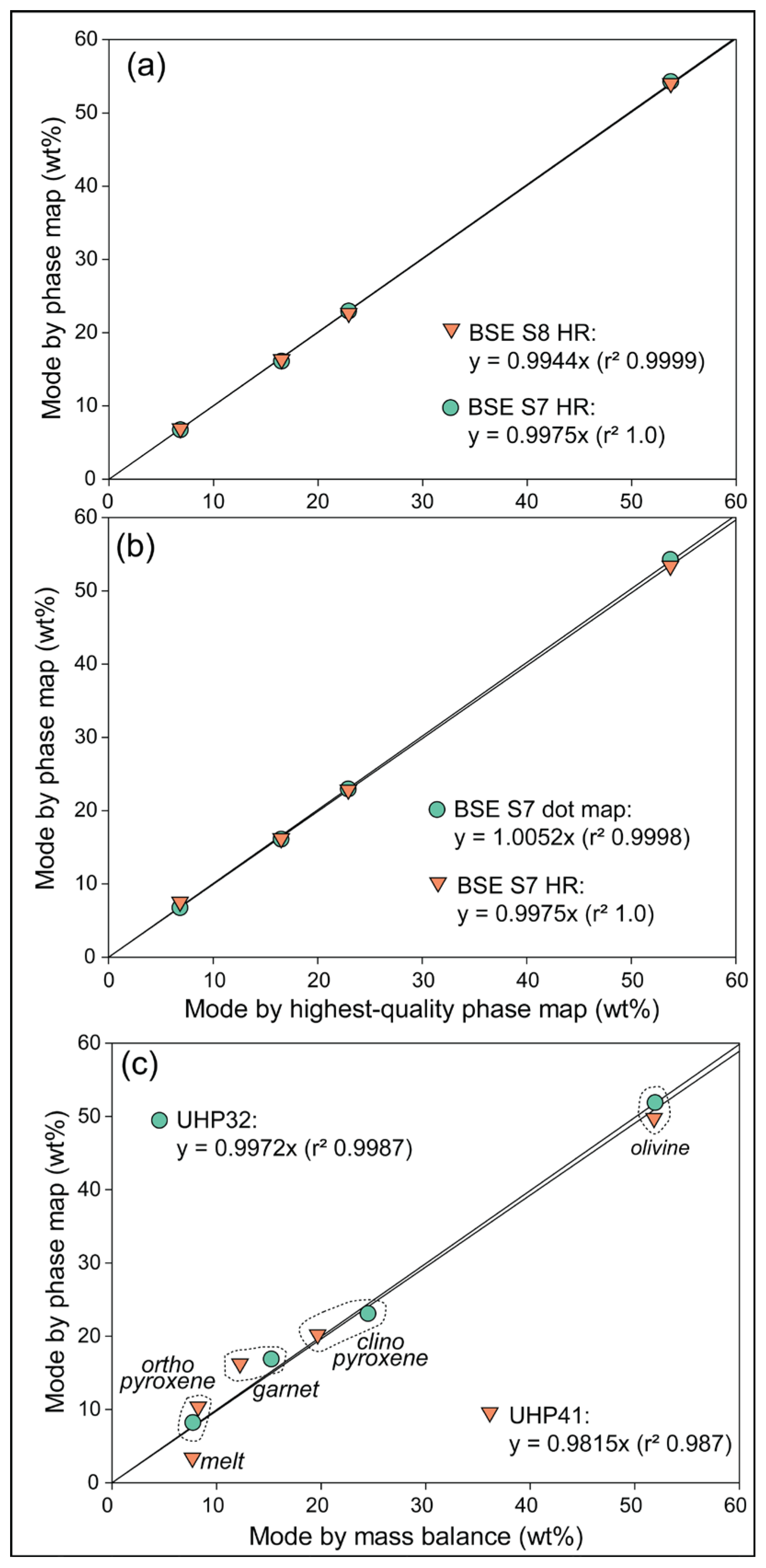
Figure 1. Schematic flow diagram explaining the image analysis steps, consecutively involving (left column, from top to bottom): acquisition > export > registration > annotation and classification > custom map analysis. Options exist to work with SEM-generated mosaic maps (this avoids image registration) and to analyze sub-regions (regions of interest ROI) on larger maps. Insert image shows a screenshot from QuPath’s interactive combined viewer in which the phase categories are annotated (yellow polygon on olivine).
Minerals 15 00355 g001
Figure 2. Details extracted from BSE frames obtained on sample UHP32, exposing olivine, clinopyroxene, garnet, and orthopyroxene. The 8 images were obtained with increasingly slow scan speeds (S3 to S10, reflecting 1, 3.2, 10, 32, 100, 320, 1000, and 3200 µs/pixel). Note that grain boundaries are becoming substantially clearer from S5 to S8 but that further improvement from S8 to S10 relates to diminishing greyscale ‘noise’ within phases rather than the sharpness of grain contacts. Also shown for comparison is a phase map (bottom right corner). The bottom panel shows grey level intensity histograms.
Minerals 15 00355 g002
Figure 3. BSE intensity profiles (16-bit) across orthopyroxene, garnet, olivine, and clinopyroxene peridotite assemblage of UHP32, shown as a phase map on the top panel and a strip of encountered phases at the bottom. In all BSE intensity profiles, the scan speed setting of interest (red traces S6, S7, S8, and S9) was compared to the slowest speed setting, S10 (as a grey line).
Minerals 15 00355 g003
Figure 4. Small area phase maps on sample UHP32. (a) was obtained with the proprietary TIMA software combining fast BSE scanning with HR EDS mapping. (b) was obtained with the open-source software approach developed for this study combining the slowest scan speed (S10) BSE image with HR EDS mapping. The areas shown in Figure 2 and Figure 3 are indicated with boxes. (c,d) both used BSE images obtained with scan speed S7 but were combined with HR (c) and dot mapping (d) EDS acquisitions.
Minerals 15 00355 g004
Figure 5. Equivalence comparison between phase map Figure 4b (true class, y-axis) with homologous phase maps Figure 4c (BSE scan speed S7 with HR EDS mapping) and Figure 4d (BSE scan speed S7 with dot EDS mapping). See text for explanation.
Minerals 15 00355 g005
Figure 6. Linear regressions of various estimates of modal abundance (all by wt%). Panels (a) and (b) use data for small trial areas on sample UHP32 (see Figure 4). Both panels show the ground-truth BSE S10 with HR EDS (Figure 4b) on the x-axis and faster acquisitions on the y-axis. Panel (c) shows modal abundance estimates for the full charge area for samples UHP32 (see Figure 7 for full phase map) and UHP40 (see Figure 8 for full phase map). The x-axis shows the mode by mass balance, and the y-axis mode by phase map (BSE S7 with EDS dot mapping).
Minerals 15 00355 g006
Figure 9. Modes, phase associations, and phase map Phase maps of sample UHP21. (a,b) show mode and mutual phase associations in ‘Zone A’ and ‘Zone B’, respectively, of the phase map (c). For statistical purposes (modal abundance and phase association), the map was subdivided into ‘Zone B’, representing lower temperature and a melt-, and orthopyroxene-rich ‘Zone B’. In ‘Zone A’ garnet and garnet-melt inclusions in olivine are annotated with ‘gi’ and ‘gmi’, respectively.
Minerals 15 00355 g009
Figure 10. Association matrices for small map area on sample UHP32 (Figure 4a,b,d) obtained with various SEM BSE and EDS settings. Note the preferential contacts between the two pyroxenes. Same color scheme as Figure 7.
Minerals 15 00355 g010
Figure 11. Thermodynamically modeled wt% modal abundance of pyroxenes and garnet in GKR-001. The x-axis shows melt fraction (wt%) generated over 23 °C, and the y-axis shows modal abundance of minerals in the solid residue (other than olivine). Over a very narrow temperature interval of 16 °C, this system is modeled to produce 16.6 wt% melt (x-axis) at the expense of clinopyroxene while also crystallizing copious peritectic orthopyroxene.
Minerals 15 00355 g011
Figure 12. Back-scattered electron montages output from TIMA (left) and AMICS version 3.3.3.0. (right) software for the same area on sample UHP32. The dashed yellow lines trace the boundaries of adjacent frames. The circles in red (TIMA) and cyan (AMICS) show the locations of small ‘stitching’ errors.
Minerals 15 00355 g012
Figure 13. (a) The left panel shows a re-registered phase map made with a transformation matrix (intensity-based registration) from exported overlapping Bruker AMICS BSE frames applied to exported phase map frames. (b) The right panel shows the new phase map generated with annotations in QuPath on combined Bruker AMICS BSE and phase maps. Note the better definition of grain boundaries of the same phase (white arrows) on the right-hand side phase map, as well as the better distinction between included and adjacent phases (red arrows highlighting garnet-olivine relationships; 1 denoting garnet inclusion, 2 denoting interstitial garnet).
Minerals 15 00355 g013
Table 1. Composition of the starting mixture (GKR-001) and run products in equilibrated charges.
GKR-001UHP32 (5 GPa, 1525 °C, 9 h)
Ol (32) 2Opx (17)Cpx (30)Grt (23)
SiO245.5240.83 (23) 356.36 (22)55.03 (23)42.37 (28)
TiO20.070.08 (06)0.04 (01)0.04 (01)0.21 (07)
Al2O34.410.17 (20)2.55 (17)2.67 (09)22.70 (60)
Cr2O30.320.09 (02)0.28 (02)0.30 (03)1.29 (23)
FeOt7.118.80 (16)5.18 (08)4.57 (15)5.66 (16)
MnO0.150.14 (01)0.13 (02)0.15 (02)0.21 (03)
MgO38.1849.97 (37)33.15 (59)25.50 (31)22.48 (20)
NiO0.100.08 (03)0.06 (02)0.05 (01)bdl
CaO3.960.30 (15)2.62 (68)11.53 (43)5.07 (26)
Na2O0.090.03 (00)0.07 (02)0.24 (01)bdl
K2O0.01bdl 1bdlbdlbdl
Total99.90100.39100.40100.0599.99
Mg#90.5491.0191.9490.8790.76
Mode (wt%)
Mass balance 51.957.7424.4815.23
Phase map 51.878.1923.0716.86
UHP40 (5 GPa, 1600 °C, 5 h)
Ol (22)Opx (29)Cpx (29)Grt (27)Melt (07) 4
SiO241.10 (22)56.12 (43)54.74 (26)42.85 (23)46.74 (97)
TiO2bdl0.03 (01)0.03 (01)0.15 (03)0.24 (07)
Al2O30.15 (02)3.11 (34)3.12 (12)22.71 (36)8.90 (1.0)
Cr2O30.10 (01)0.32 (03)0.35 (02)1.36 (22)0.44 (04)
FeOt8.21 (13)4.93 (09)4.56 (14)5.22 (16)11.11 (02)
MnO0.13 (01)0.12 (01)0.15 (01)0.20 (02)0.17 (01)
MgO50.24 (28)32.98 (32)26.74 (56)22.71 (24)18.00 (1.2)
NiO0.02 (01)0.03 (01)0.02 (00)bdlbdl
CaO0.28 (01)2.56 (18)9.79 (69)4.95 (22)13.95 (07)
Na2O0.02 (01)0.07 (01)0.21 (02)bdl0.45 (02)
K2Obdlbdlbdlbdl0.01 (00)
Total100.32100.2499.69100.15100.00
Mg#91.5092.2691.2790.2774.27
Mode (wt%)
Mass balance51.848.2419.6612.237.69
Phase map49.7810.3720.2216.243.38
1 bdl = below detection limit. 2 Number of analyses. 3 Standard deviation of “n” analyses of each phase in each experimental run product. 4 Melt composition was normalized to 100%.
Disclaimer/Publisher’s Note: The statements, opinions and data contained in all publications are solely those of the individual author(s) and contributor(s) and not of MDPI and/or the editor(s). MDPI and/or the editor(s) disclaim responsibility for any injury to people or property resulting from any ideas, methods, instructions or products referred to in the content.

