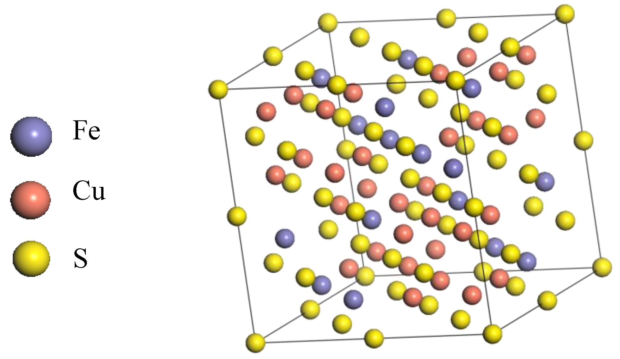
Figure 1.
The structure of F-43m bornite in DFT calculation.
Figure 1.
The structure of F-43m bornite in DFT calculation.
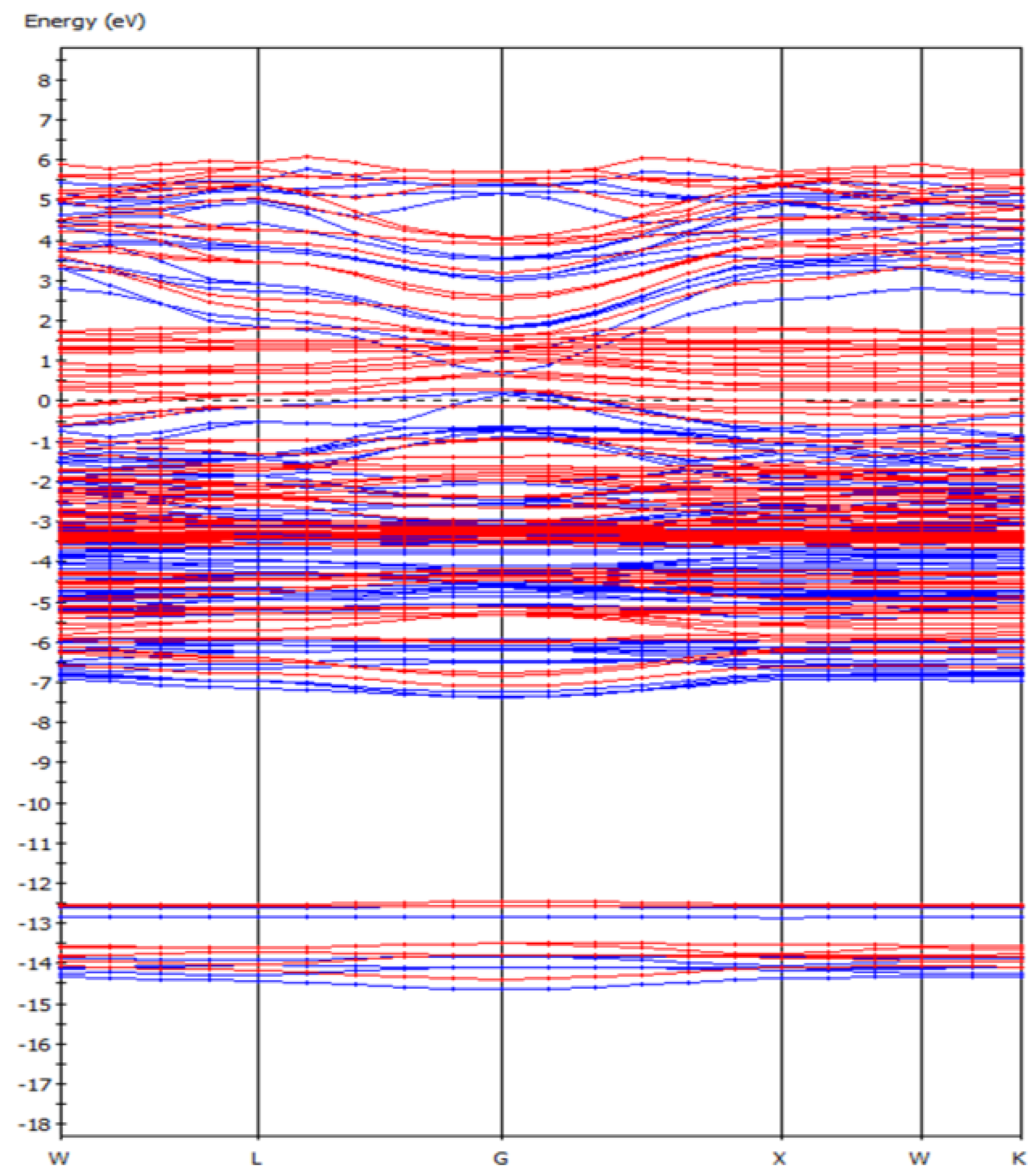
Figure 2.
The band structure of bornite (X-axis, High symmetry point; Y-axis, Energy/eV) in DFT calculation (CASTEP module of Materials Studio 6.0 software package, PBE density function, Hubbard + U correction).
Figure 2.
The band structure of bornite (X-axis, High symmetry point; Y-axis, Energy/eV) in DFT calculation (CASTEP module of Materials Studio 6.0 software package, PBE density function, Hubbard + U correction).
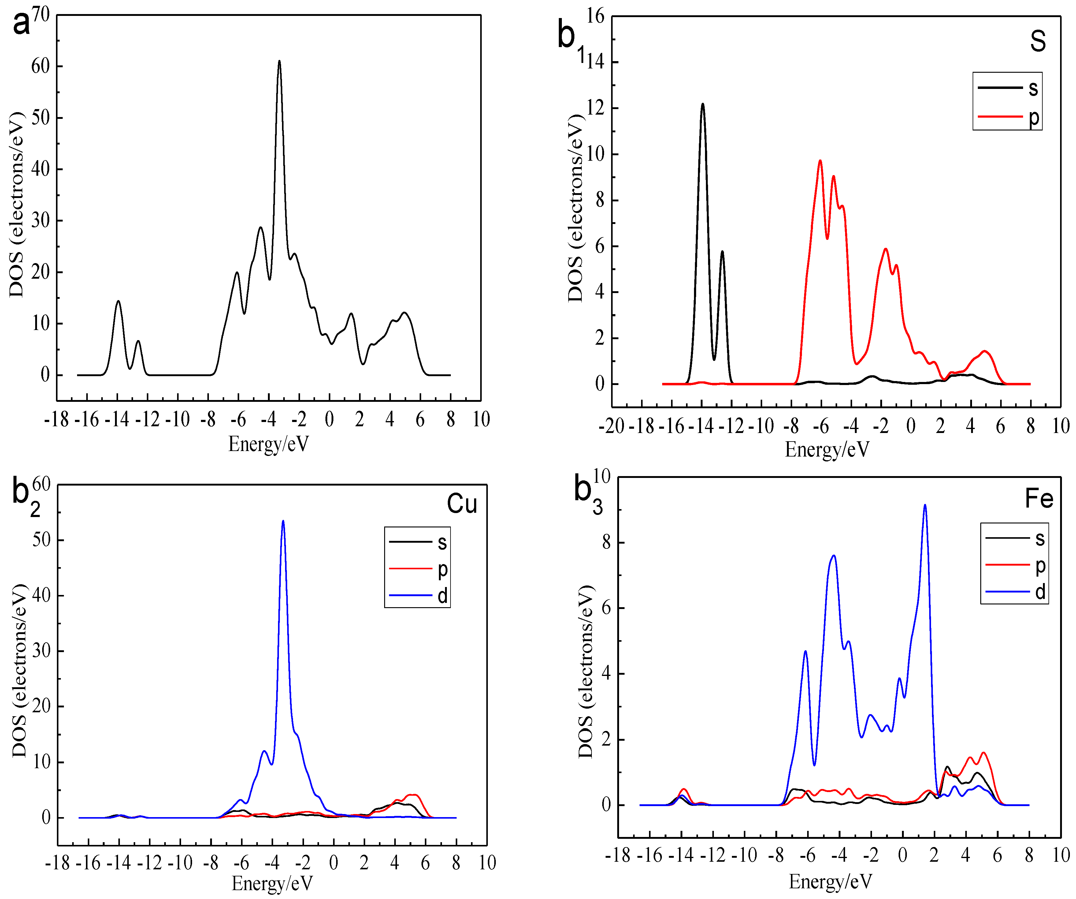
Figure 3.
DOS and PDOS of bornite in DFT calculation (CASTEP module of Materials Studio 6.0 software package, PBE density function, Hubbard + U correction): (a) Total; (b1) Cu; (b2) Fe; (b3) S.
Figure 3.
DOS and PDOS of bornite in DFT calculation (CASTEP module of Materials Studio 6.0 software package, PBE density function, Hubbard + U correction): (a) Total; (b1) Cu; (b2) Fe; (b3) S.
Figure 4.
Reconstruction of bornite (111)-S surface in DFT calculation (CASTEP module of Materials Studio 6.0 software package, PBE density function, Hubbard + U correction): (a1) Top and (a2) side views of optimized (111)-S surface; (b1) Top and (b2) side views of initial (111)-S surface.
Figure 4.
Reconstruction of bornite (111)-S surface in DFT calculation (CASTEP module of Materials Studio 6.0 software package, PBE density function, Hubbard + U correction): (a1) Top and (a2) side views of optimized (111)-S surface; (b1) Top and (b2) side views of initial (111)-S surface.
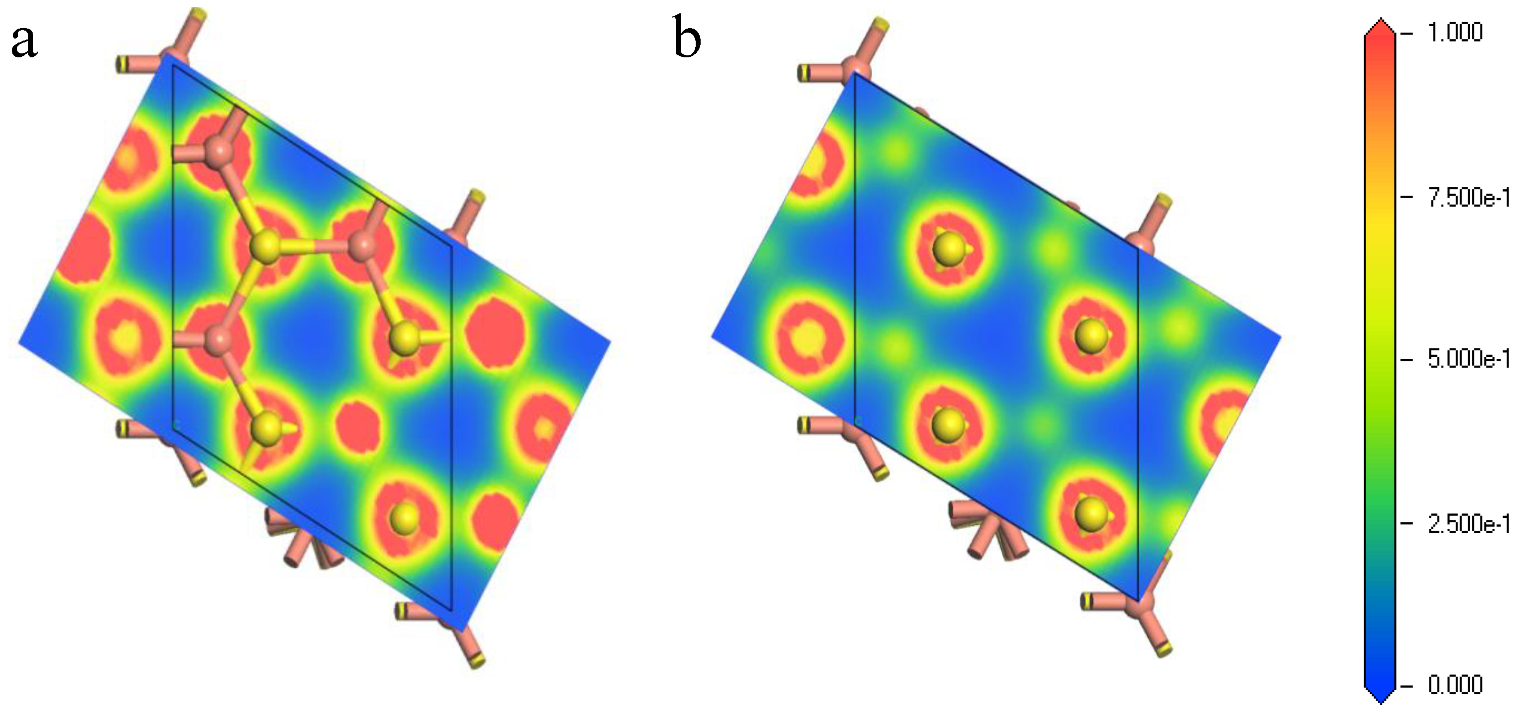
Figure 5.
Electron density of bornite (111)-S surface before and after reconstruction in DFT calculation (CASTEP module of Materials Studio 6.0 software package, PBE density function, Hubbard + U correction): (a) The first layer of optimized (111)-S surface; (b) The first layer of initial (111)-S surface.
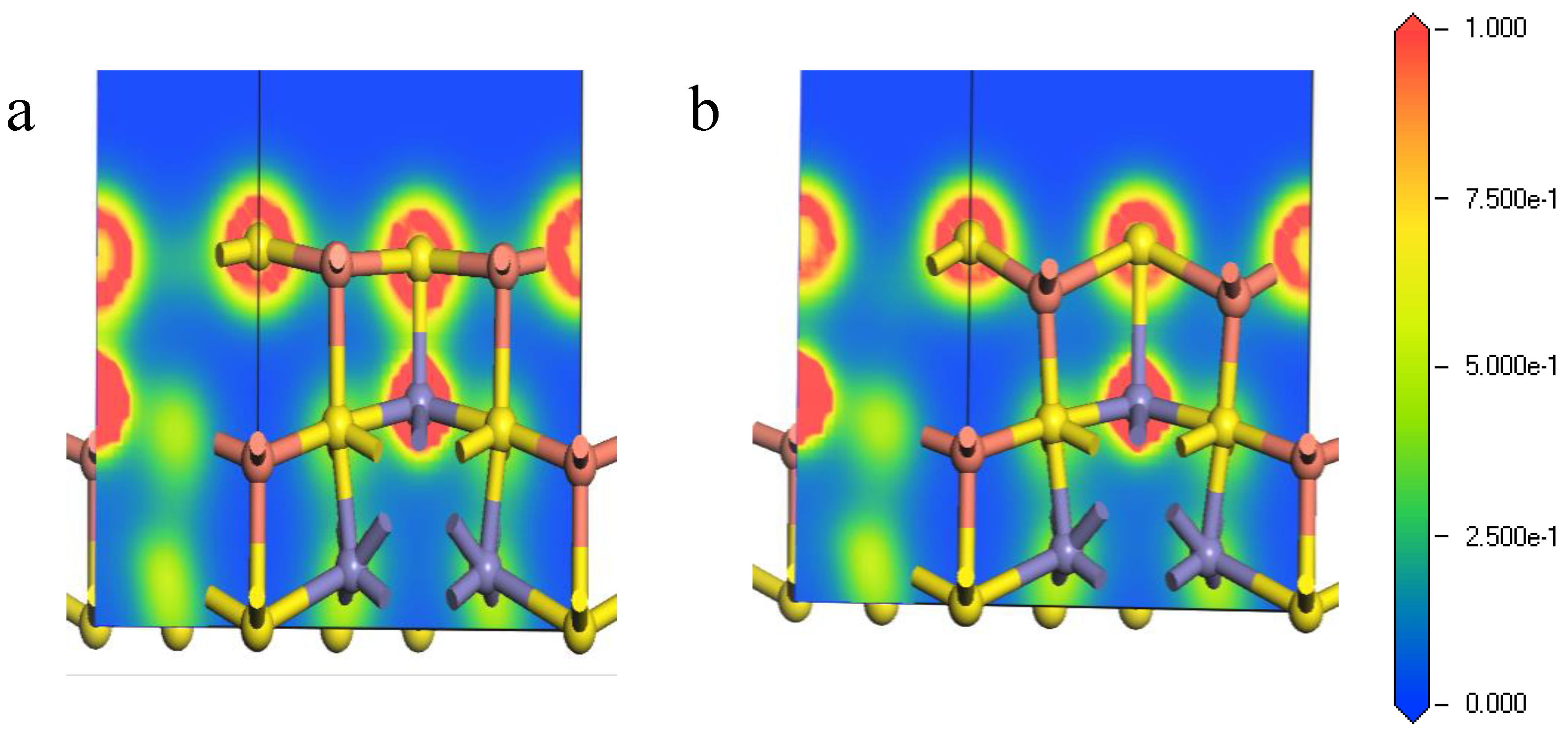
Figure 6.
Electron density of Fe-S bond of bornite (111)-S surface before and after reconstruction in DFT calculation (CASTEP module of Materials Studio 6.0 software package, PBE density function, Hubbard + U correction): (a) The optimized Fe-S bond; (b) The initial Fe-S bond.
Figure 6.
Electron density of Fe-S bond of bornite (111)-S surface before and after reconstruction in DFT calculation (CASTEP module of Materials Studio 6.0 software package, PBE density function, Hubbard + U correction): (a) The optimized Fe-S bond; (b) The initial Fe-S bond.
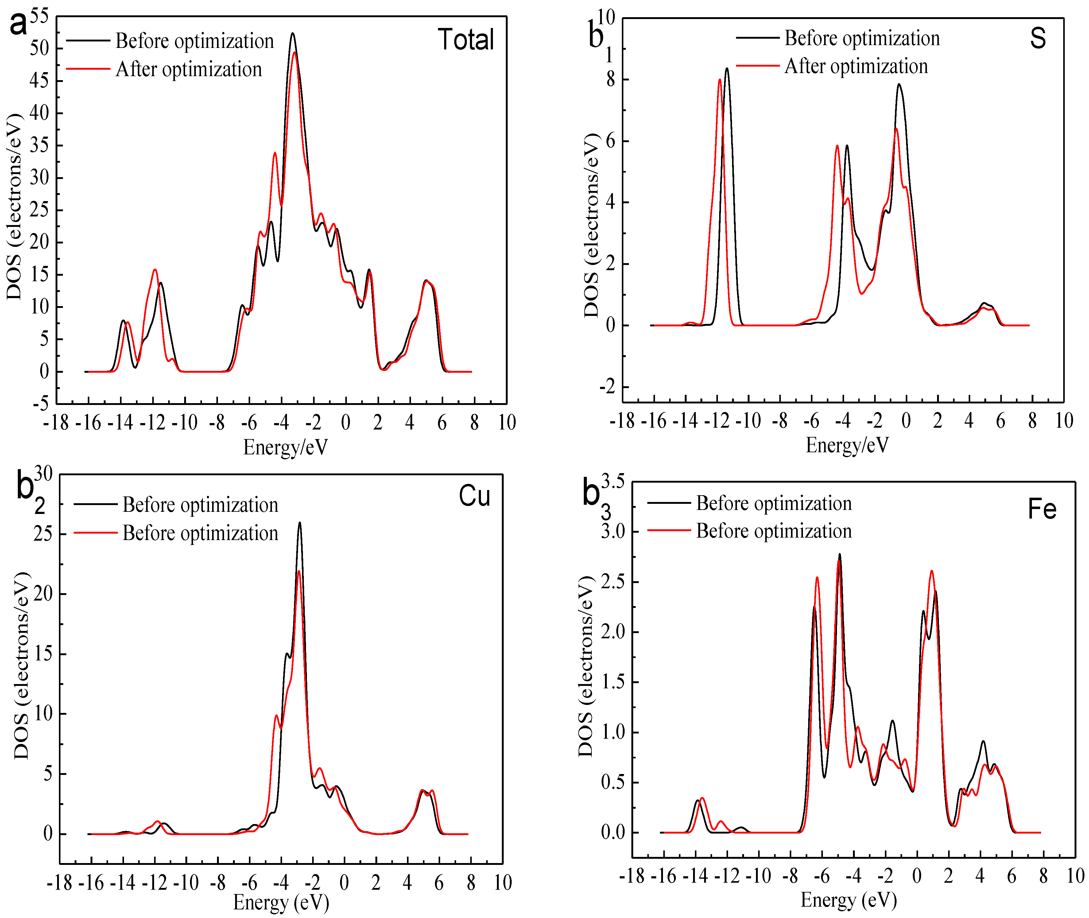
Figure 7.
Local DOS of bornite before and after optimization (CASTEP module of Materials Studio 6.0 software package, PBE density function, Hubbard + U correction): (a) Total; (b1) S; (b2) Cu; (b3) Fe in DFT calculation.
Figure 7.
Local DOS of bornite before and after optimization (CASTEP module of Materials Studio 6.0 software package, PBE density function, Hubbard + U correction): (a) Total; (b1) S; (b2) Cu; (b3) Fe in DFT calculation.
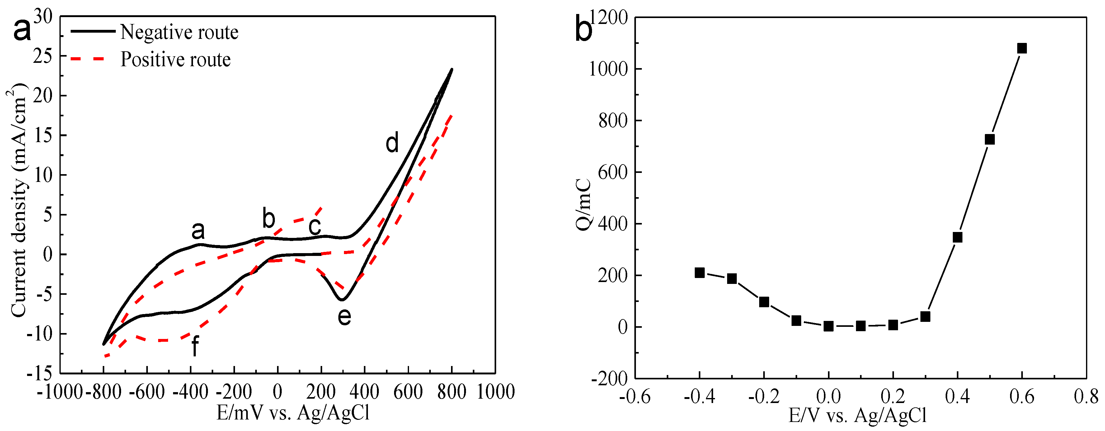
Figure 8.
Electrochemistry analysis of bornite in 9K bacterial culture medium (Conventional three-electrode system on a Princeton Model 283 Potentiostat, EG&G of Princeton Applied Research): (a) Cyclic voltammograms of bornite electrode (Scan rate 20 mV/s); (b) Relationship between the total charges (evaluated from the current-time curves with duration time of 240 s) and applied potentials.
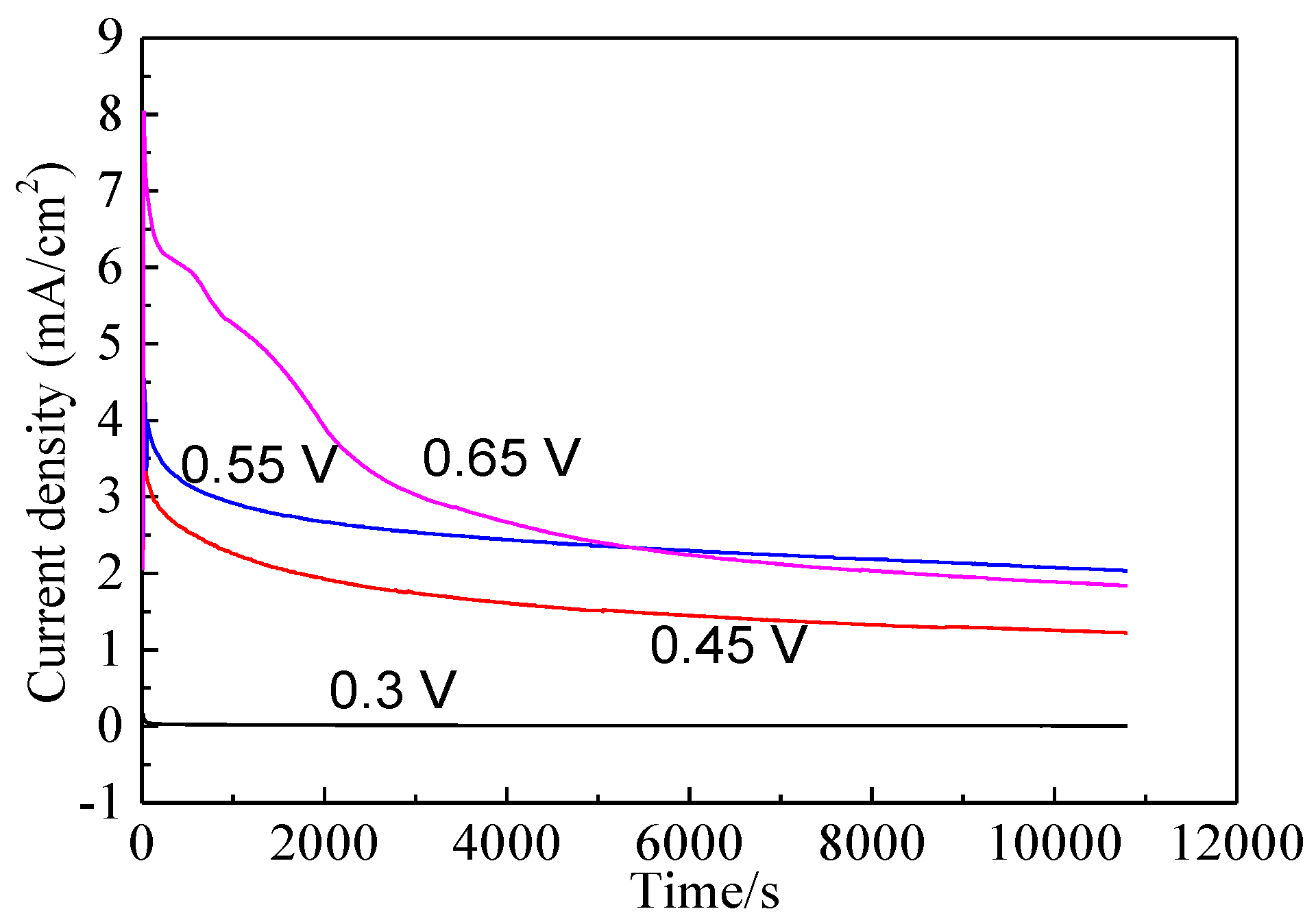
Figure 9.
Current-time curves of bornite electrode at different applied potentials for 3 h in 9K bacterial culture medium (Conventional three-electrode system on a Princeton Model 283 Potentiostat, EG&G of Princeton Applied Research).
Figure 9.
Current-time curves of bornite electrode at different applied potentials for 3 h in 9K bacterial culture medium (Conventional three-electrode system on a Princeton Model 283 Potentiostat, EG&G of Princeton Applied Research).
Figure 10.
The open circuit potential of bornite electrode after treating by different potentials for 3 h in 9K bacterial culture medium (Conventional three-electrode system on a Princeton Model 283 Potentiostat, EG&G of Princeton Applied Research).
Figure 10.
The open circuit potential of bornite electrode after treating by different potentials for 3 h in 9K bacterial culture medium (Conventional three-electrode system on a Princeton Model 283 Potentiostat, EG&G of Princeton Applied Research).
Figure 11.
XPS spectra of Cu peaks of bornite surface after treating by different potential of 0, 0.3, 0.45, 0.55, 0.65 V, respectively: (a) Cu 2p peak; (b) Cu LMM peak (Implemented on the model of ESCALAB 250Xi of Al Kα X-ray source with 20 eV constant pass energy and 0.1 eV/step; Fitted by Thermo Avantage 5.52, C 1s 284.8 eV as reference, Shirley method, Gaussian-Lorentzian function).
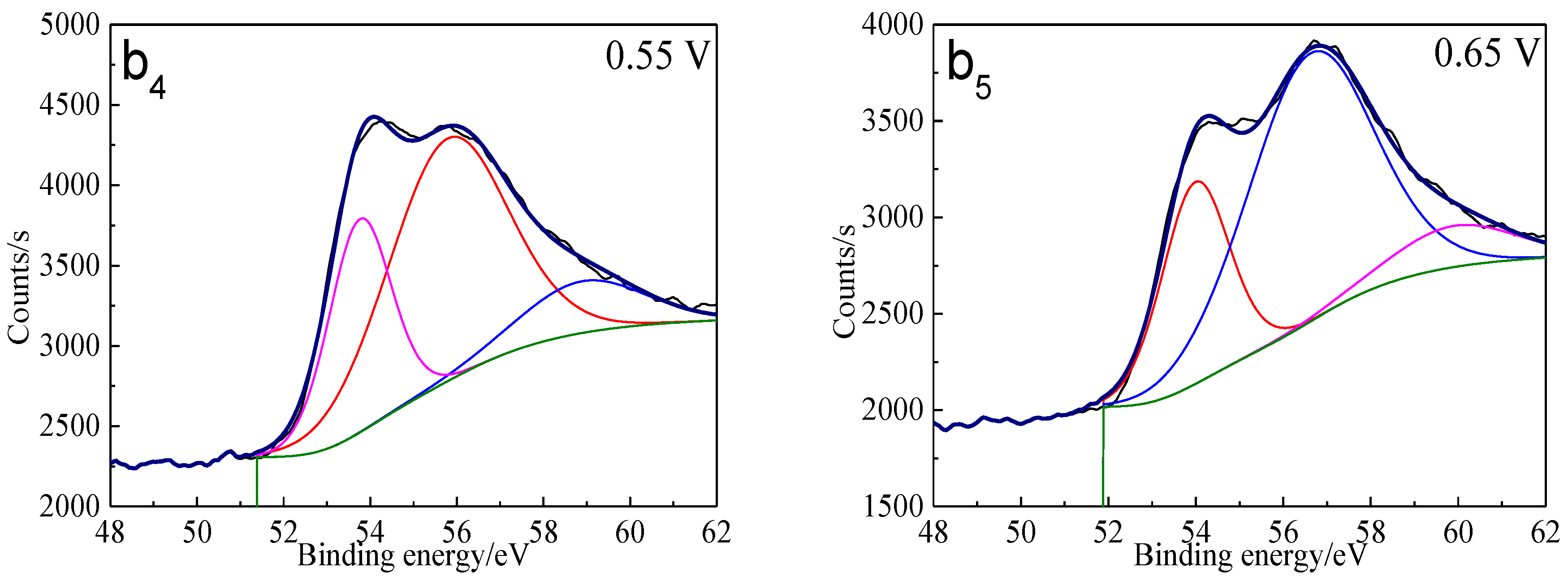
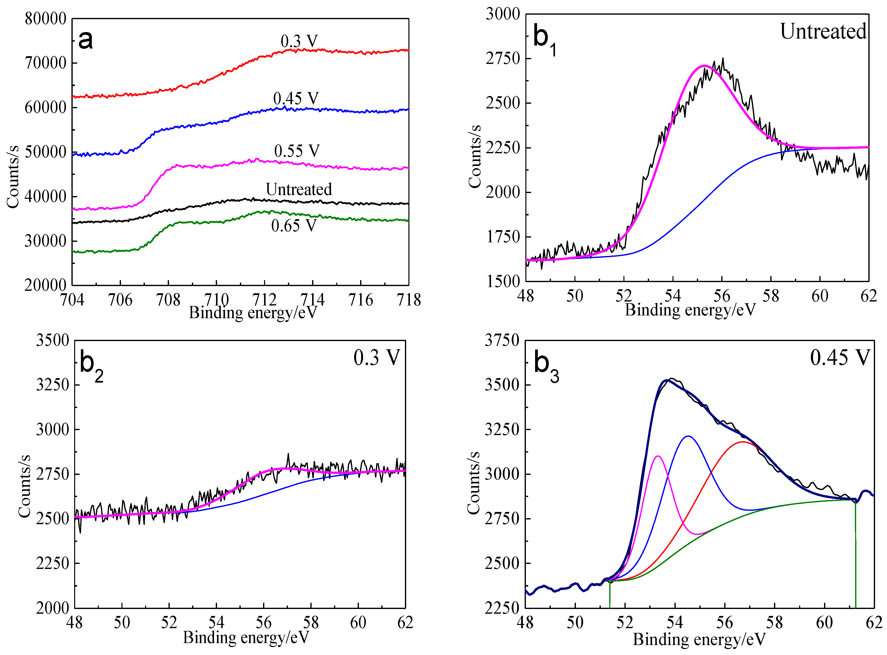
Figure 12.
XPS spectra of Fe peaks of bornite surface after treating by different potential of 0, 0.3, 0.45, 0.55, 0.65 V, respectively: (a) Fe 2p peak; (b1–b5): Fe 3p peak (Implemented on the model of ESCALAB 250Xi of Al Kα X-ray source with 20 eV constant pass energy and 0.1 eV/step; Fitted by Thermo Avantage 5.52, C 1s 284.8 eV as reference, Shirley method, Gaussian-Lorentzian function).
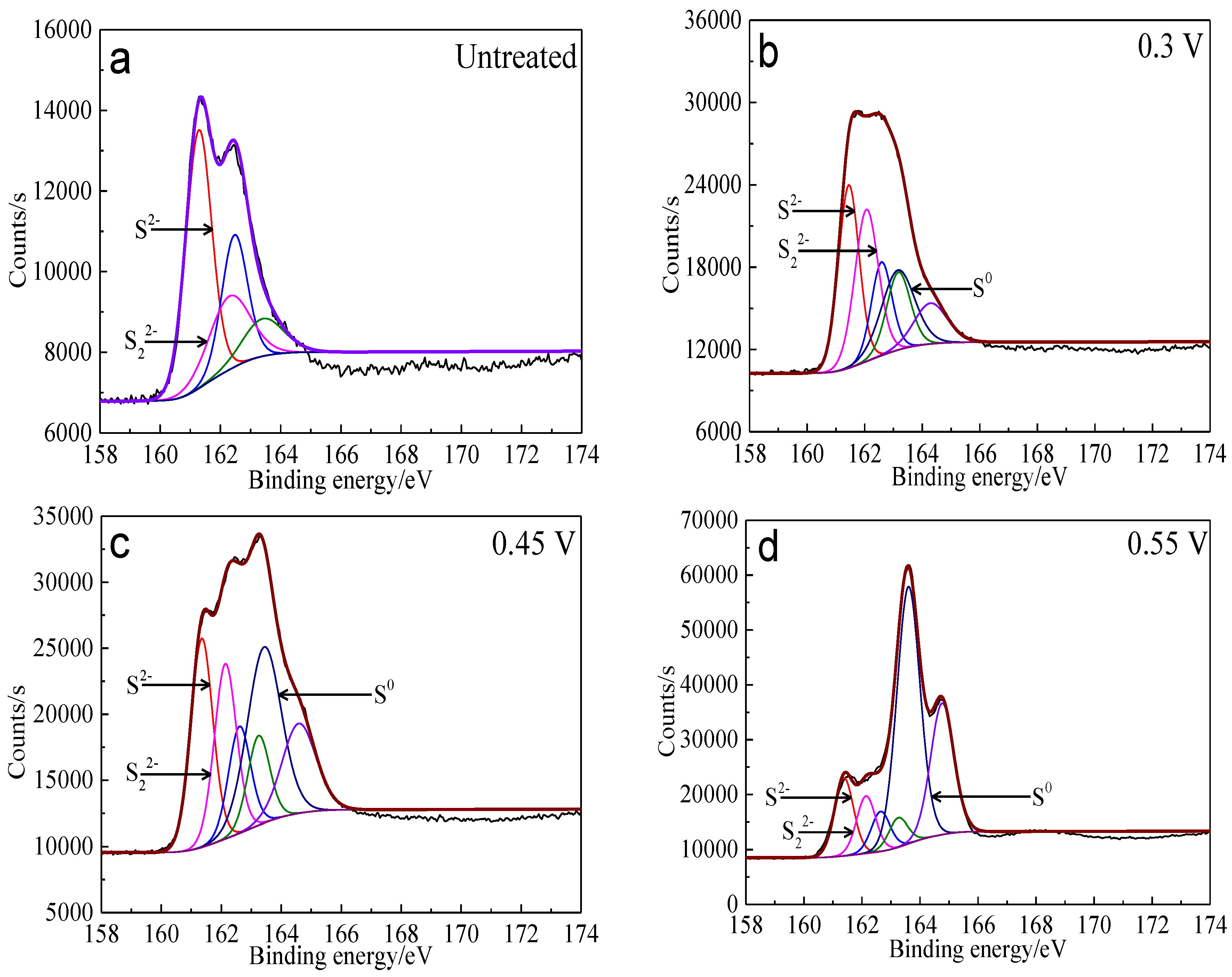
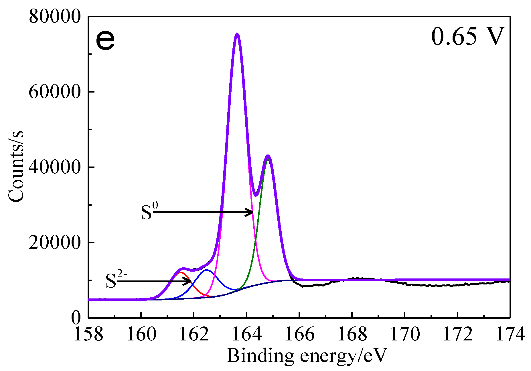
Figure 13.
XPS spectra of S 2p peaks of bornite surface after treating by different potential of 0, 0.3, 0.45, 0.55, 0.65 V, respectively: (a) Untreated; (b) 0.3 V; (c) 0.45 V; (d) 0.55 V; (e) 0.65V (Implemented on the model of ESCALAB 250Xi of Al Kα X-ray source with 20 eV constant pass energy and 0.1 eV/step; Fitted by Thermo Avantage 5.52, C 1s 284.8 eV as reference, Shirley method, Gaussian-Lorentzian function).
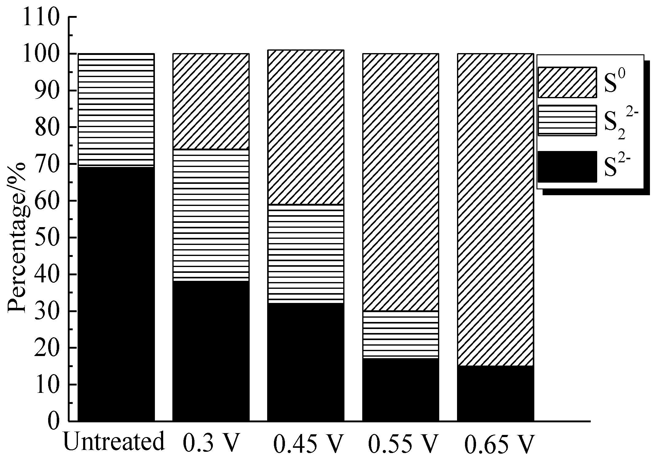
Figure 14.
Distribution of sulfur containing species on bornite surface after treating by different potential of 0, 0.3, 0.45, 0.55, 0.65 V, respectively (Implemented on the model of ESCALAB 250Xi of Al Kα X-ray source with 20 eV constant pass energy and 0.1 eV/step; Fitted by Thermo Avantage 5.52, C 1s 284.8 eV as reference, Shirley method, Gaussian-Lorentzian function).
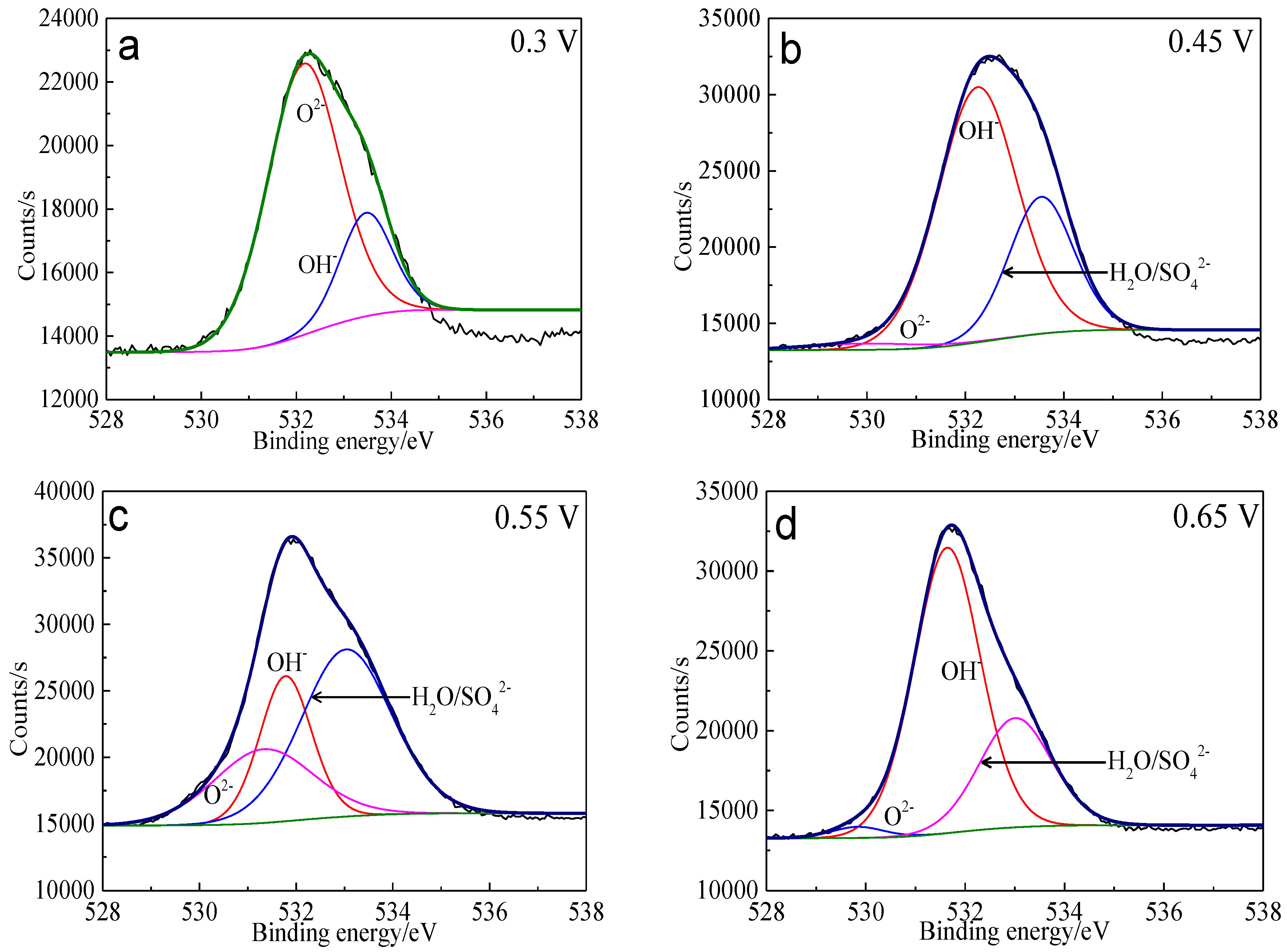
Figure 15.
XPS spectra of O 1s peaks of bornite surface after treating by different potential of 0, 0.3, 0.45, 0.55, 0.65 V, respectively: (a) 0.3 V; (b) 0.45 V; (c) 0.55 V; (d) 0.65 V (Implemented on the model of ESCALAB 250Xi of Al Kα X-ray source with 20 eV constant pass energy and 0.1 eV/step; Fitted by Thermo Avantage 5.52, C 1s 284.8 eV as reference, Shirley method, Gaussian-Lorentzian function).
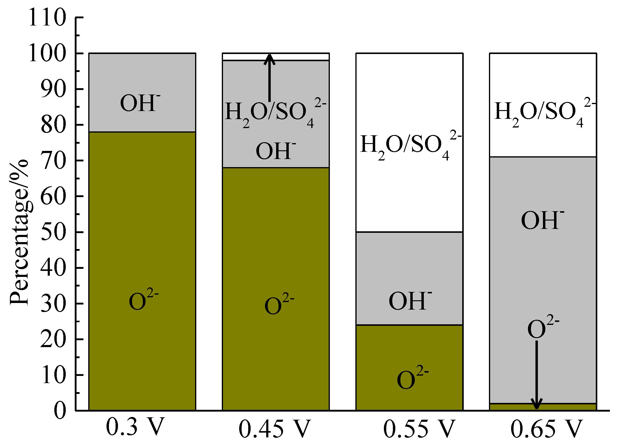
Figure 16.
Distribution of oxygen containing species on bornite surface after treating by different potential of 0, 0.3, 0.45, 0.55, 0.65 V, respectively (Implemented on the model of ESCALAB 250Xi of Al Kα X-ray source with 20 eV constant pass energy and 0.1 eV/step; Fitted by Thermo Avantage 5.52, C 1s 284.8 eV as reference, Shirley method, Gaussian-Lorentzian function).
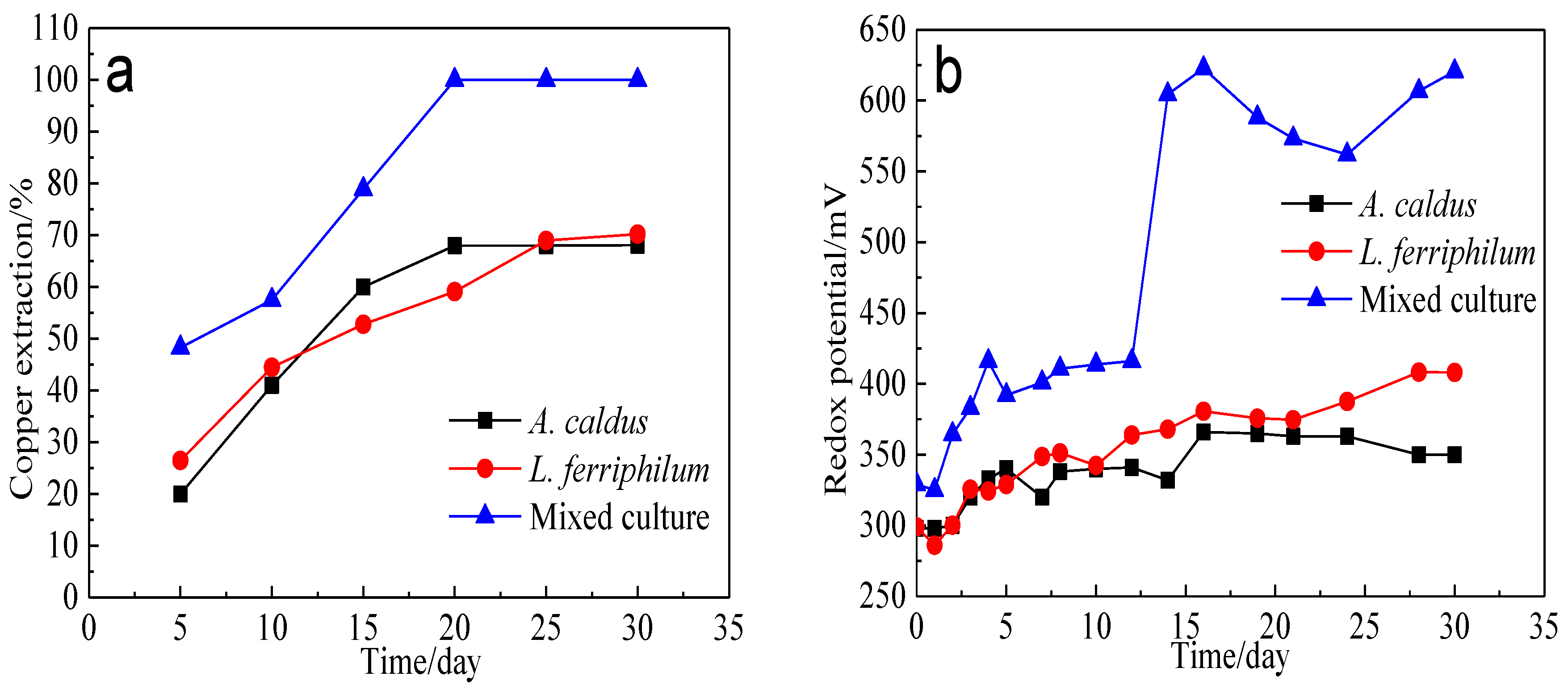
Figure 17.
Bioleaching of bornite by A. caldus, L. ferriphilum and mixed culture consisting of A. caldus and L. ferriphilum: (a) Copper extraction; (b) Redox potential.
Figure 17.
Bioleaching of bornite by A. caldus, L. ferriphilum and mixed culture consisting of A. caldus and L. ferriphilum: (a) Copper extraction; (b) Redox potential.
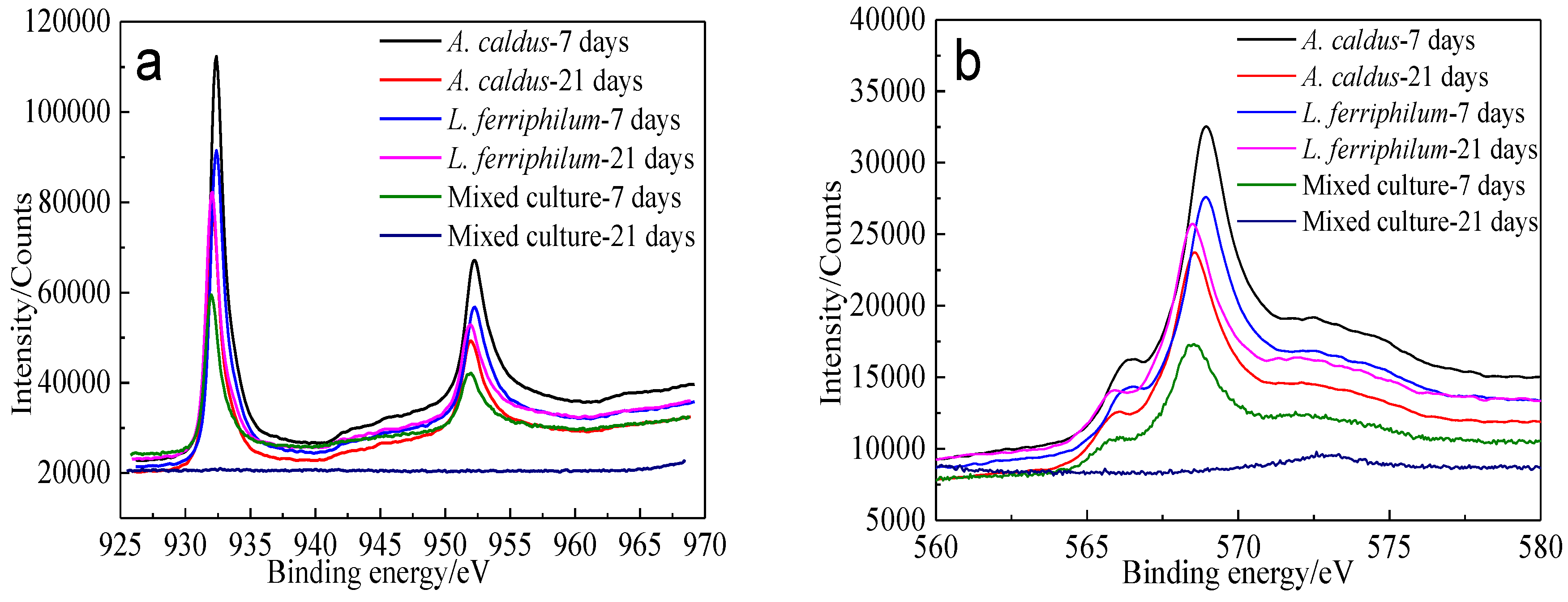
Figure 18.
XPS spectra of Cu peaks of bornite surface leached by A. caldus, L. ferriphilum and mixed culture consisting of A. caldus and L. ferriphilum for 7 and 21 days, respectively (Implemented on the model of ESCALAB 250Xi of Al Kα X-ray source with 20 eV constant pass energy and 0.1 eV/step; Fitted by Thermo Avantage 5.52, C 1s 284.8 eV as reference, Shirley method, Gaussian-Lorentzian function): (a) Cu 2p peak; (b) Cu LMM peak.
Figure 19.
XPS spectra of S 2p peaks of bornite surface leached by A. caldus, L. ferriphilum and mixed culture consisting of A. caldus and L. ferriphilum for 7 and 21 days, respectively (Implemented on the model of ESCALAB 250Xi of Al Kα X-ray source with 20 eV constant pass energy and 0.1 eV/step; Fitted by Thermo Avantage 5.52, C 1s 284.8 eV as reference, Shirley method, Gaussian-Lorentzian function): (a1)-A. caldus and 7 days; (a2)-A. caldus and 21 days; (b1)-L. ferriphilum and 7 days; (b2)-L. ferriphilum and 21 days; (c1)-mixed culture and 7 days; (c2)-mixed culture and 21 days.
Figure 20.
Distribution of sulfur containing species on bornite surface leached by A. caldus, L. ferriphilum and mixed culture consisting of A. caldus and L. ferriphilum for 7 and 21 days, respectively (Implemented on the model of ESCALAB 250Xi of Al Kα X-ray source with 20 eV constant pass energy and 0.1 eV/step; Fitted by Thermo Avantage 5.52, C 1s 284.8 eV as reference, Shirley method, Gaussian-Lorentzian function).
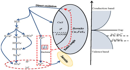
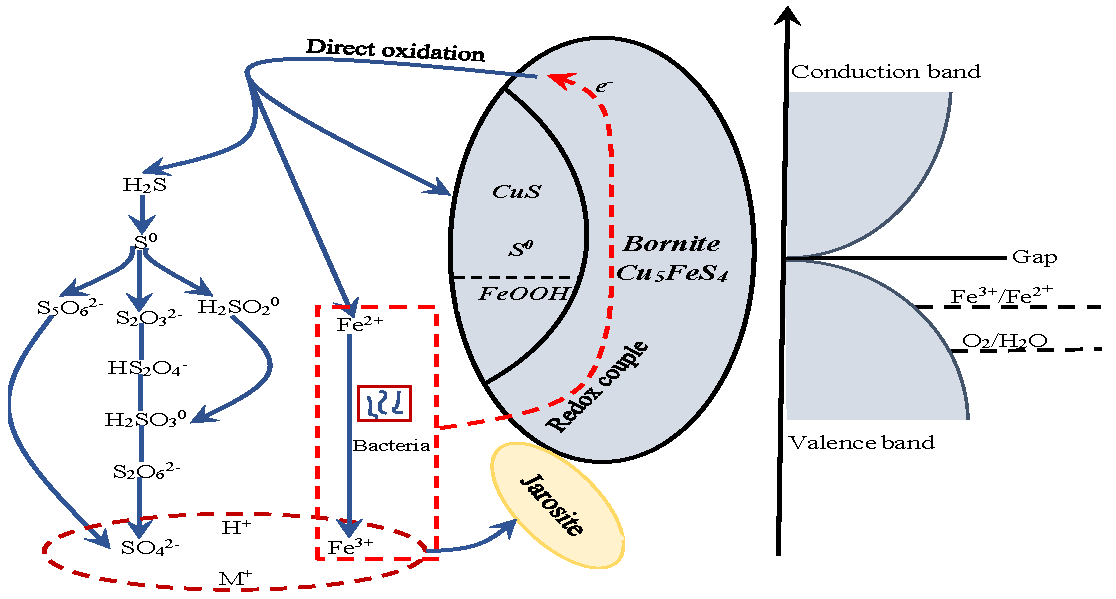
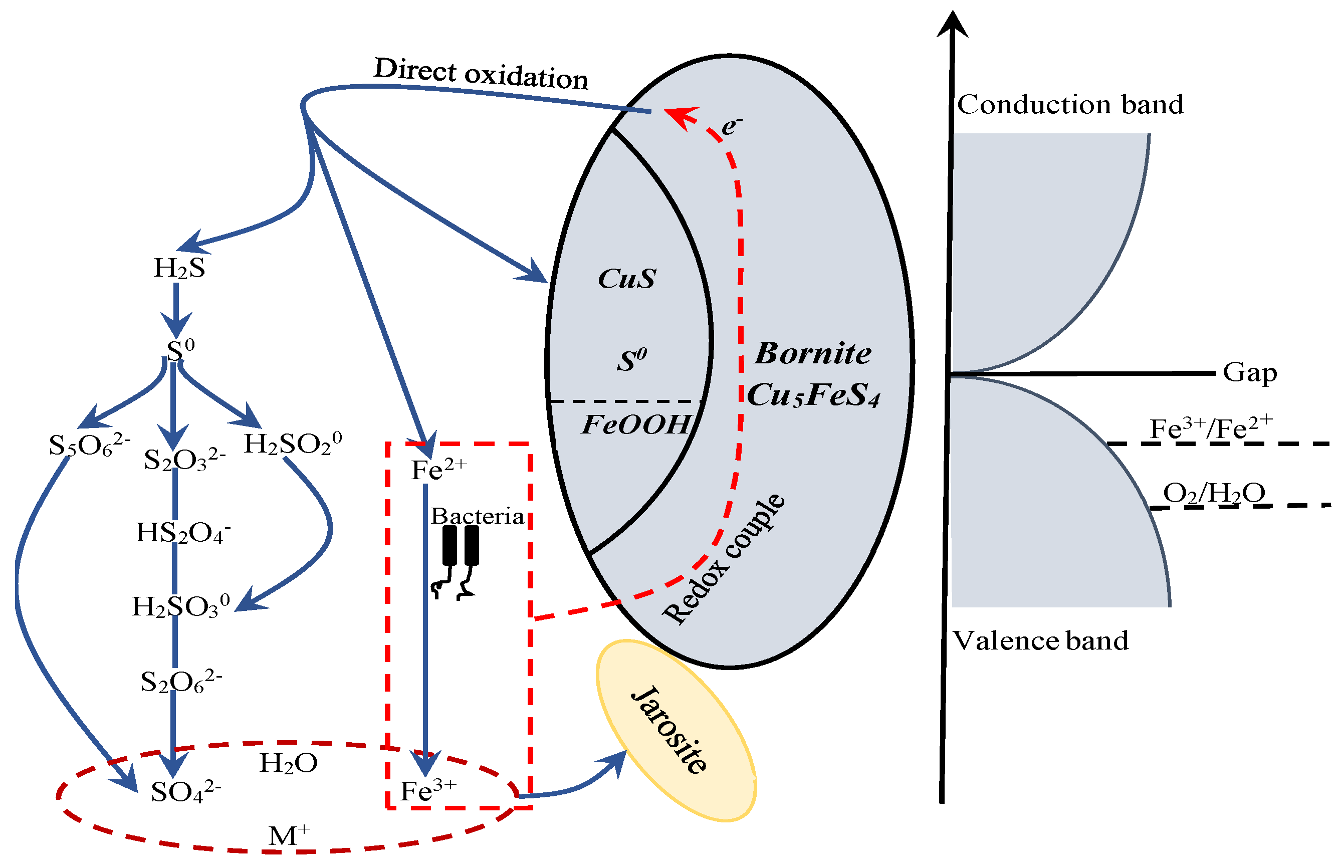
Figure 21.
The proposed model for interpreting the dissolution process of bornite in bioleaching by moderately thermophilic microorganisms.
Figure 21.
The proposed model for interpreting the dissolution process of bornite in bioleaching by moderately thermophilic microorganisms.
Table 1.
Lattice constants of the bornite structure in DFT calculation (CASTEP module of Materials Studio 6.0 software package, PBE density function, Hubbard + U correction).
Table 1.
Lattice constants of the bornite structure in DFT calculation (CASTEP module of Materials Studio 6.0 software package, PBE density function, Hubbard + U correction).
| Crystal System | Space Groups | Lattice Constant | Crystal Angle |
|---|
| Cubic | F-43m | a = b = c = 10.710 Å | α = β = γ = 90° |
Table 2.
Convergence test results of energy cut-off in DFT calculation (CASTEP module of Materials Studio 6.0 software package, PBE density function, Hubbard + U correction).
Table 2.
Convergence test results of energy cut-off in DFT calculation (CASTEP module of Materials Studio 6.0 software package, PBE density function, Hubbard + U correction).
| Cut-off Energy/eV | SCF Loops | dEtot/dlog (Ecut) | Final Energy/eV |
|---|
| 390 | 115 | - | −17,491.94660 |
| 395 | 15 | - | −17,491.94830 |
| 400 | 15 | −0.15371 | −17,491.95020 |
Table 3.
Results of cell parameters optimization in DFT calculation and reference (CASTEP module of Materials Studio 6.0 software package, PBE density function, Hubbard + U correction).
Table 3.
Results of cell parameters optimization in DFT calculation and reference (CASTEP module of Materials Studio 6.0 software package, PBE density function, Hubbard + U correction).
| Parameter | Reference | Optimization Result | Relative Error/% |
|---|
| a = b = c | 10.710 Å | 11.0503 Å | 3.2 |
| α = β = γ | 90° | 90° | - |
Table 4.
Mulliken population of bornite in DFT calculation (CASTEP module of Materials Studio 6.0 software package, PBE density function, Hubbard + U correction).
Table 4.
Mulliken population of bornite in DFT calculation (CASTEP module of Materials Studio 6.0 software package, PBE density function, Hubbard + U correction).
| Species | Ion | s | p | d | Total | Charge/e | Spin/hbar |
|---|
| S | 1 | 1.79 | 4.56 | 0.00 | 6.34 | −0.34 | 0.04 |
| S | 2 | 1.85 | 4.54 | 0.00 | 6.39 | −0.39 | 0.13 |
| S | 3 | 1.79 | 4.55 | 0.00 | 6.33 | −0.33 | 0.12 |
| S | 4 | 1.79 | 4.55 | 0.00 | 6.34 | −0.34 | 0.10 |
| S | 5 | 1.79 | 4.55 | 0.00 | 6.33 | −0.33 | 0.12 |
| S | 6 | 1.79 | 4.55 | 0.00 | 6.34 | −0.34 | 0.10 |
| S | 7 | 1.79 | 4.55 | 0.00 | 6.33 | −0.33 | 0.12 |
| S | 8 | 1.79 | 4.55 | 0.00 | 6.34 | −0.34 | 0.10 |
| Fe | 1 | 0.36 | 0.64 | 6.54 | 7.54 | 0.46 | 1.70 |
| Fe | 2 | 0.36 | 0.64 | 6.54 | 7.54 | 0.46 | 1.70 |
| Fe | 3 | 0.36 | 0.64 | 6.54 | 7.54 | 0.46 | 1.70 |
| Fe | 4 | 0.34 | 0.60 | 6.54 | 7.54 | 0.46 | 1.67 |
| Cu | 1 | 0.60 | 0.56 | 6.54 | 10.95 | 0.05 | 0.00 |
| Cu | 2 | 0.59 | 0.55 | 6.60 | 10.94 | 0.06 | 0.00 |
| Cu | 3 | 0.59 | 0.55 | 9.79 | 10.94 | 0.06 | 0.00 |
| Cu | 4 | 0.59 | 0.55 | 9.79 | 10.94 | 0.06 | 0.00 |
| Cu | 5 | 0.49 | 0.50 | 9.79 | 10.82 | 0.18 | 0.04 |
| Cu | 6 | 0.50 | 0.50 | 9.79 | 10.83 | 0.17 | 0.04 |
| Cu | 7 | 0.50 | 0.50 | 9.84 | 10.83 | 0.17 | 0.04 |
| Cu | 8 | 0.50 | 0.50 | 9.83 | 10.83 | 0.17 | 0.04 |
Table 5.
Binding energy and FWHM value for XPS spectra of S 2p3/2 peaks of bornite after treating by different potential of 0, 0.3, 0.45, 0.55, 0.65 V, respectively (Implemented on the model of ESCALAB 250Xi of Al Kα X-ray source with 20 eV constant pass energy and 0.1 eV/step; Fitted by Thermo Avantage 5.52, C 1s 284.8 eV as reference, Shirley method, Gaussian-Lorentzian function) (FWHM means full width at half maximum, B.E. means binding energy value).
| Conditions (vs. Ag/AgCl) | Peak 1 | Peak 2 | Peak 3 |
|---|
| B.E. (eV) | B.E. (eV) | B.E. (eV) | FWHM (eV) |
|---|
| 0 V | 161.3 | 162.3 | - | - |
| 0.3 V | 161.4 | 162.1 | 163.2 | 1.4 |
| 0.45 V | 161.4 | 162.2 | 163.4 | 1.4 |
| 0.55 V | 161.4 | 162.2 | 163.6 | 1.0 |
| 0.65 V | 161.5 | - | 163.6 | 1.0 |
Table 6.
Binding energy and FWHM value for XPS spectra of S 2p3/2 peaks of bornite leached by A. caldus, L. ferriphilum and mixed culture consisting of A. caldus and L. ferriphilum for 7 and 21 days, respectively (Implemented on the model of ESCALAB 250Xi of Al Kα X-ray source with 20 eV constant pass energy and 0.1 eV/step; Fitted by Thermo Avantage 5.52, C 1s 284.8 eV as reference, Shirley method, Gaussian-Lorentzian function) (FWHM means full width at half maximum, B.E. means binding energy).
| Conditions | Time | Peak 1 | Peak 2 | Peak 3 | Peak 4 |
|---|
| /days | B.E. (eV) | FWHM (eV) | B.E. (eV) | FWHM (eV) | B.E. (eV) | FWHM (eV) | B.E. (eV) | FWHM (eV) |
|---|
| A. caldus | 7 | 161.4 | 0.7 | 162.3 | 0.9 | 163.8 | 1.4 | - | - |
| 21 | 161.2 | 0.9 | 162.1 | 0.8 | 163.5 | 1.4 | - | - |
| L. ferriphilum | 7 | 161.4 | 0.7 | 162.3 | 0.9 | 163.7 | 1.4 | - | - |
| 21 | 161.0 | 0.7 | 162.0 | 0.9 | 163.4 | 1.4 | 168.4 | 1.5 |
| Mixed culture | 7 | 161.1 | 0.8 | 162.0 | 0.9 | 163.1 | 1.0 | 168.5 | 1.1 |
| 21 | - | - | - | - | - | - | 168.6 | 1.3 |


 ,
, 


