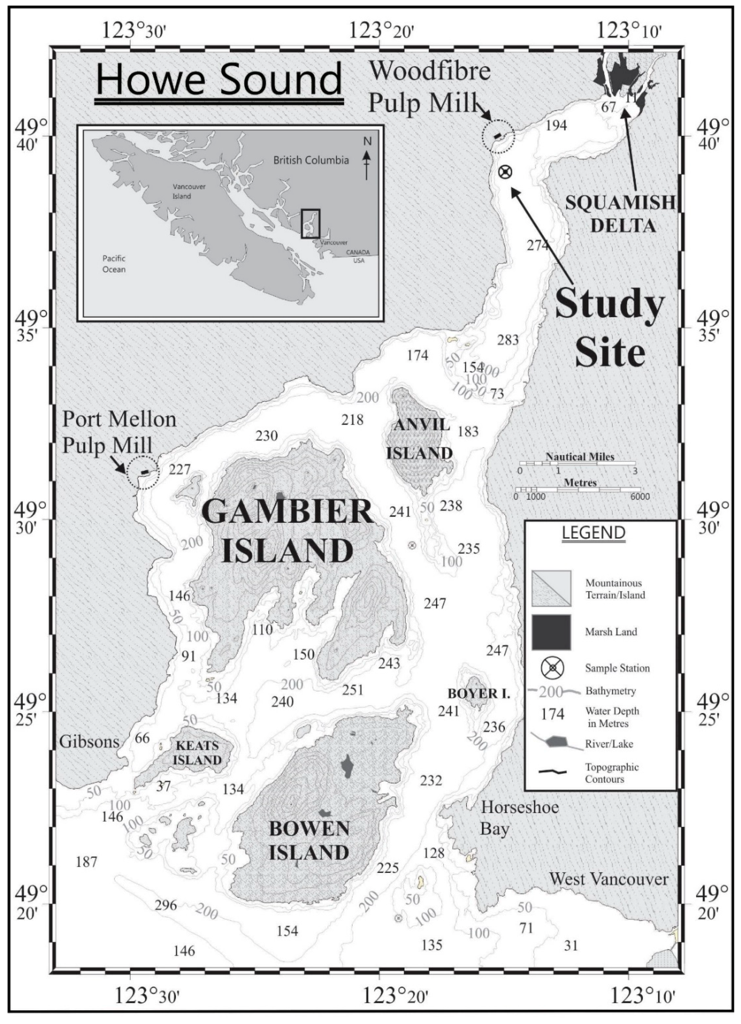
Figure 1.
Map showing the location of the sample site in Howe Sound, BC, Canada.
Figure 1.
Map showing the location of the sample site in Howe Sound, BC, Canada.
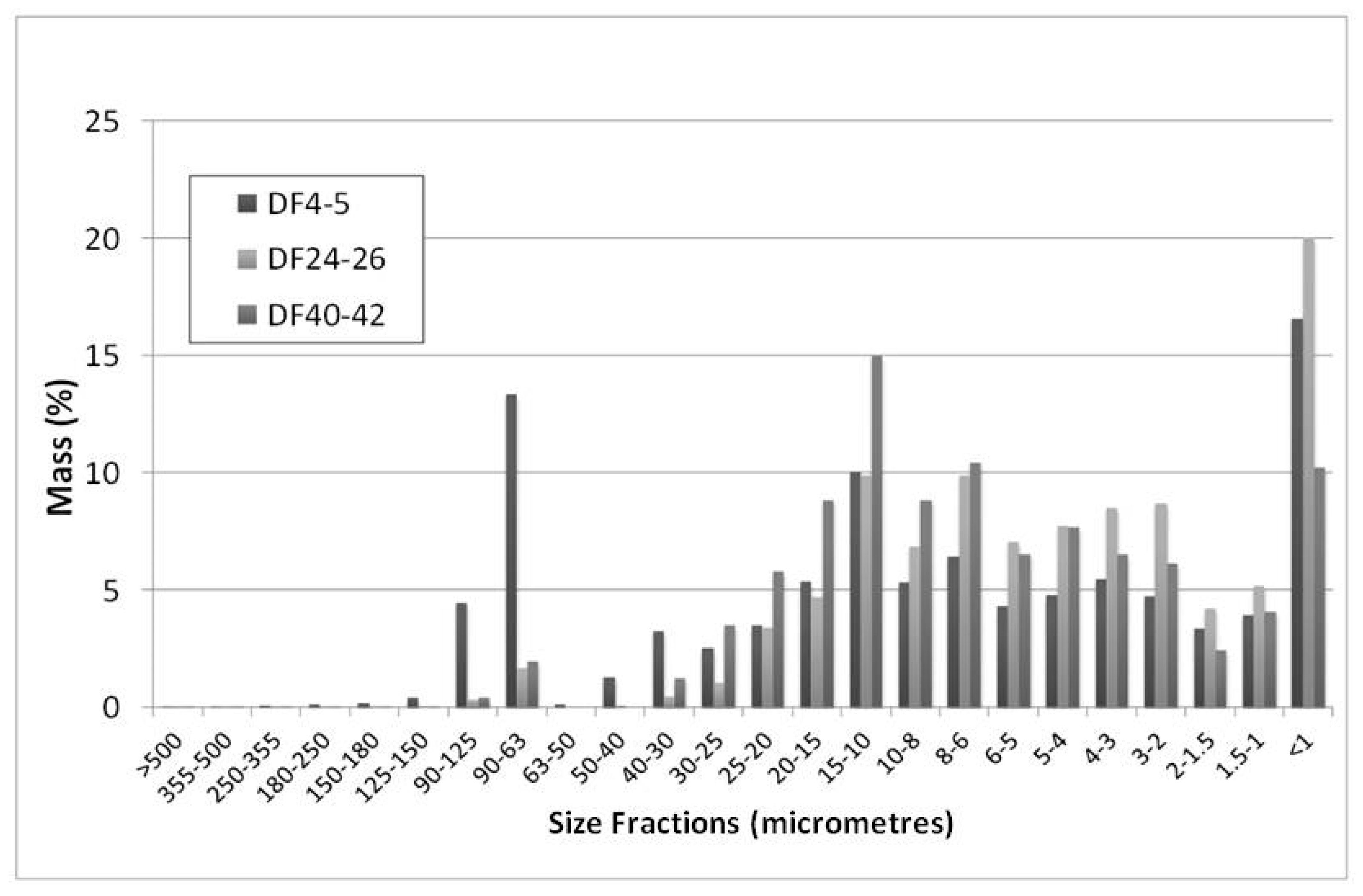
Figure 2.
Mass distribution (%) of three samples (DF 4-5, DF 24-26, DF 40-42), used to select grain size classes (micrometres) for analyses on size fractionated sediments.
Figure 2.
Mass distribution (%) of three samples (DF 4-5, DF 24-26, DF 40-42), used to select grain size classes (micrometres) for analyses on size fractionated sediments.
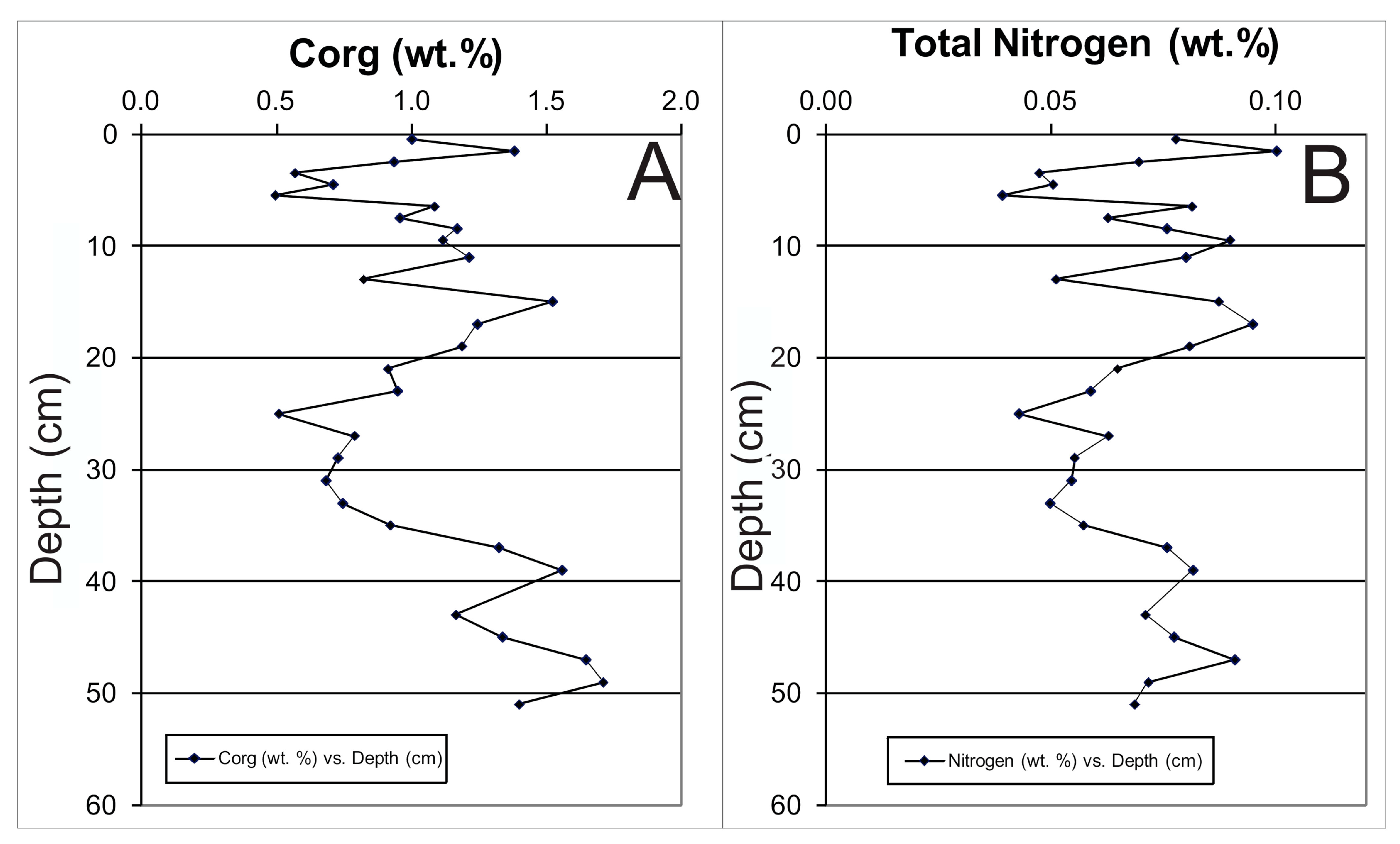
Figure 3.
Downcore variations in Organic Carbon (Corg; A) and Total Nitrogen (B) for bulk sediment samples. Both Organic carbon and Total Nitrogen concentrations show similar trends with concentration highs at the base of the cored sediment (50 cm depth) which then decrease to approximately 30 cm core depth. Concentrations of Corg and TN both increase from 30 cm to 18 cm and then fluctuate towards the sediment-water interface (0 cm depth).
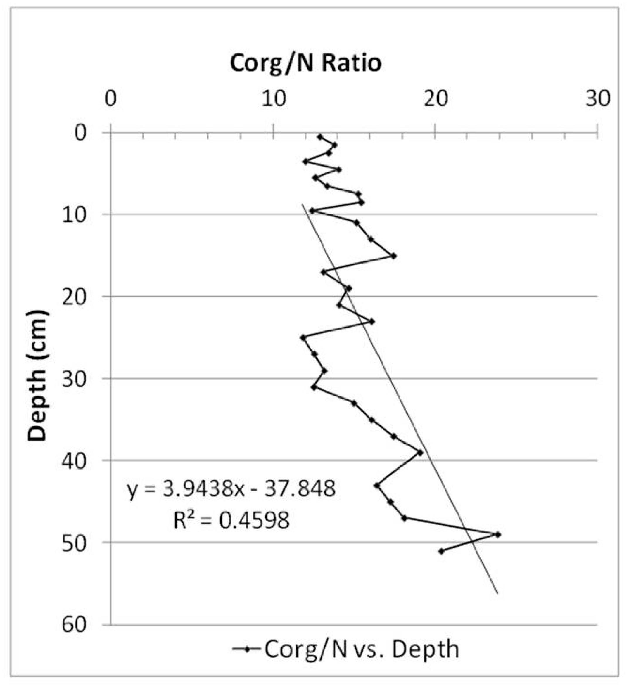
Figure 4.
Downcore variation in Organic Carbon/Total Nitrogen ratio (Corg/N). The trend line depicts a gradual increase in Corg/N ration with increasing sediment depth.
Figure 4.
Downcore variation in Organic Carbon/Total Nitrogen ratio (Corg/N). The trend line depicts a gradual increase in Corg/N ration with increasing sediment depth.
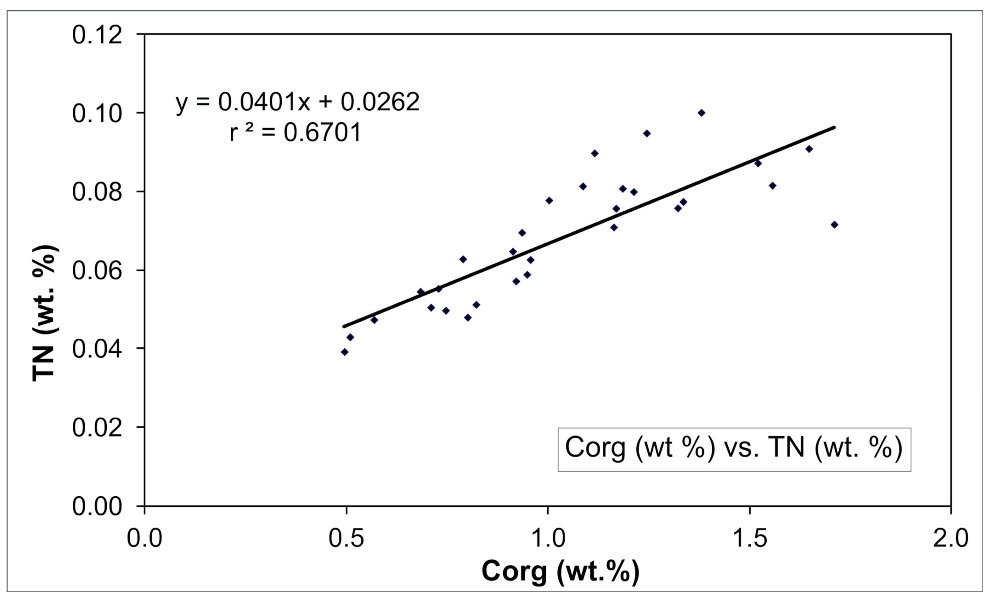
Figure 5.
Plot of Organic Carbon (Corg) versus Total Nitrogen (TN) for bulk sediment samples. A positive correlation exists between the two parameters, modeled by a linear regression (r2 = 0. 7).
Figure 5.
Plot of Organic Carbon (Corg) versus Total Nitrogen (TN) for bulk sediment samples. A positive correlation exists between the two parameters, modeled by a linear regression (r2 = 0. 7).
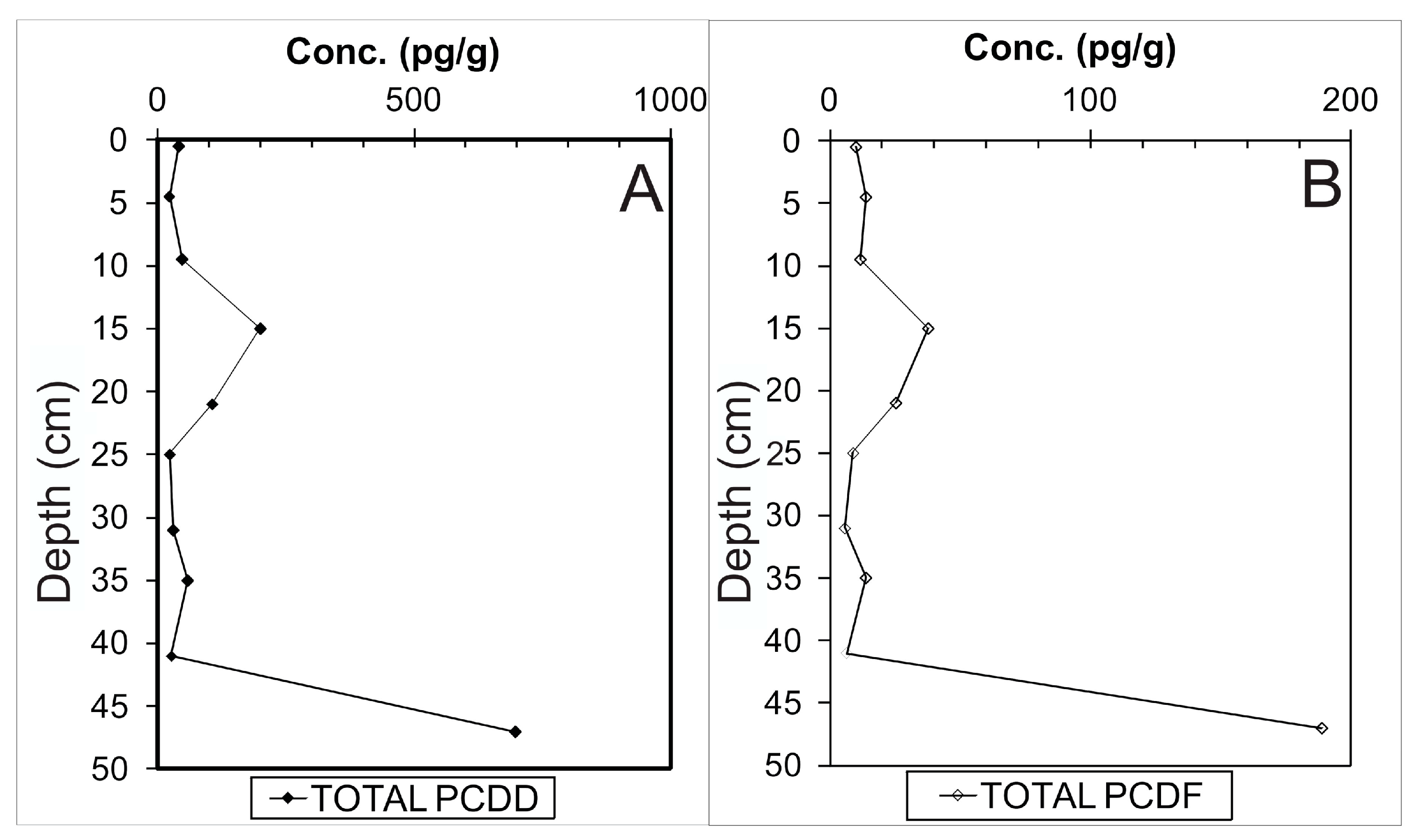
Figure 6.
Downcore variation in Total Polychlorinated Dibenzo-p-dioxin (PCDD; A) and Total Polychlorinated Dibenzo-p-furan (PCDF; B) for bulk sediment samples.
Figure 6.
Downcore variation in Total Polychlorinated Dibenzo-p-dioxin (PCDD; A) and Total Polychlorinated Dibenzo-p-furan (PCDF; B) for bulk sediment samples.
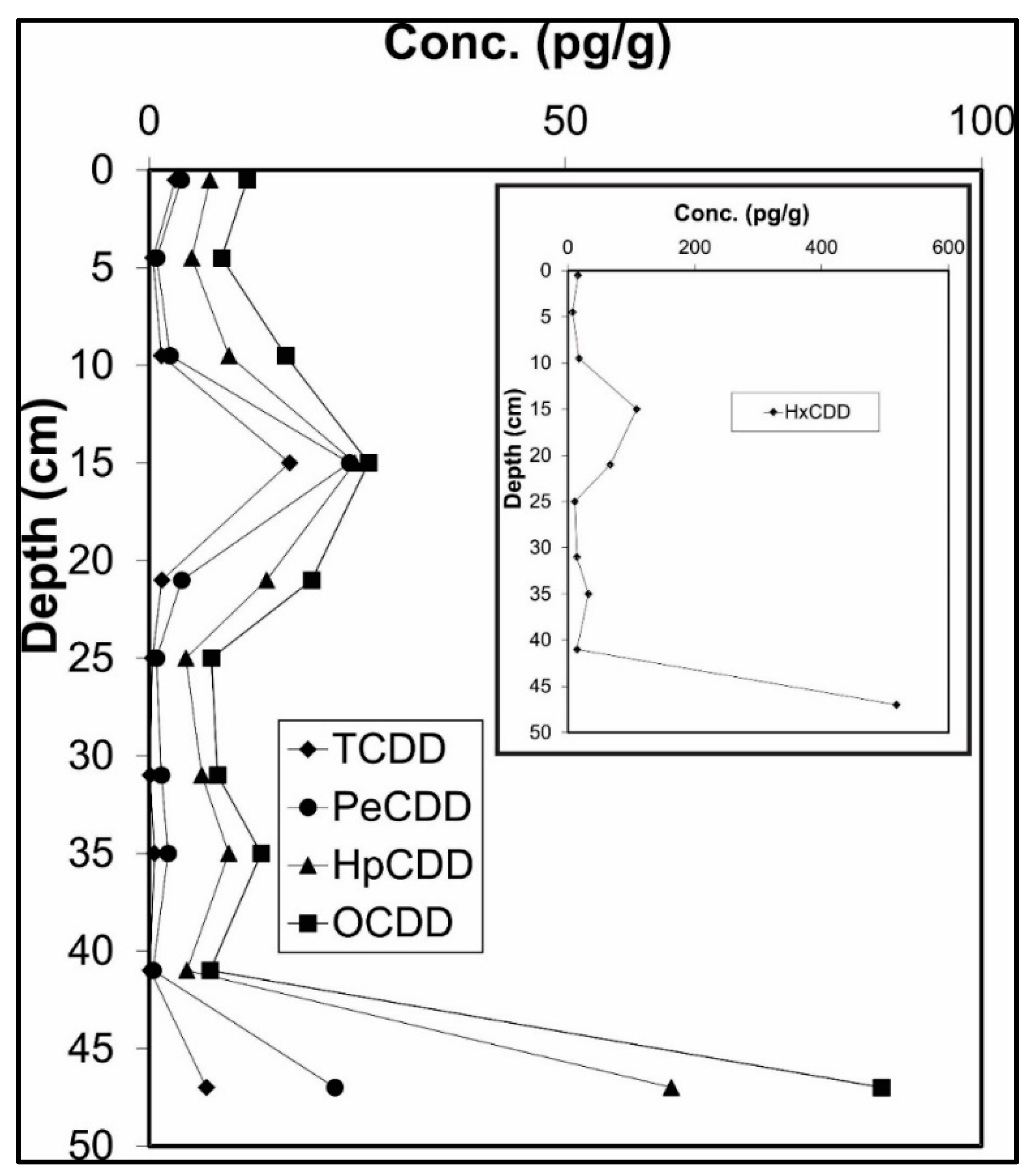
Figure 7.
Downcore variation in dioxin homologue concentration for bulk sediment samples. Inset shows HxCDD, which is present at significantly higher concentrations than the other homologues.
Figure 7.
Downcore variation in dioxin homologue concentration for bulk sediment samples. Inset shows HxCDD, which is present at significantly higher concentrations than the other homologues.
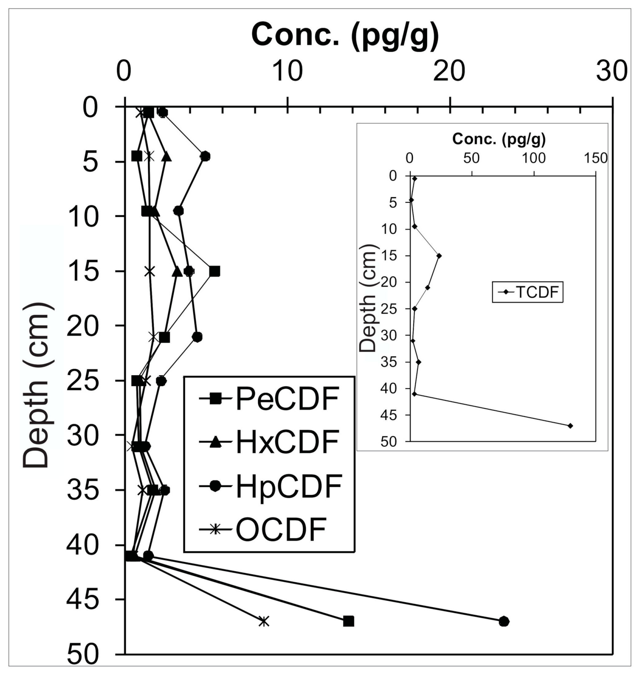
Figure 8.
Downcore variation in furan homologue concentration for bulk sediment samples. Inset shows TCDF, which is present at significantly higher concentrations than the other homologues.
Figure 8.
Downcore variation in furan homologue concentration for bulk sediment samples. Inset shows TCDF, which is present at significantly higher concentrations than the other homologues.
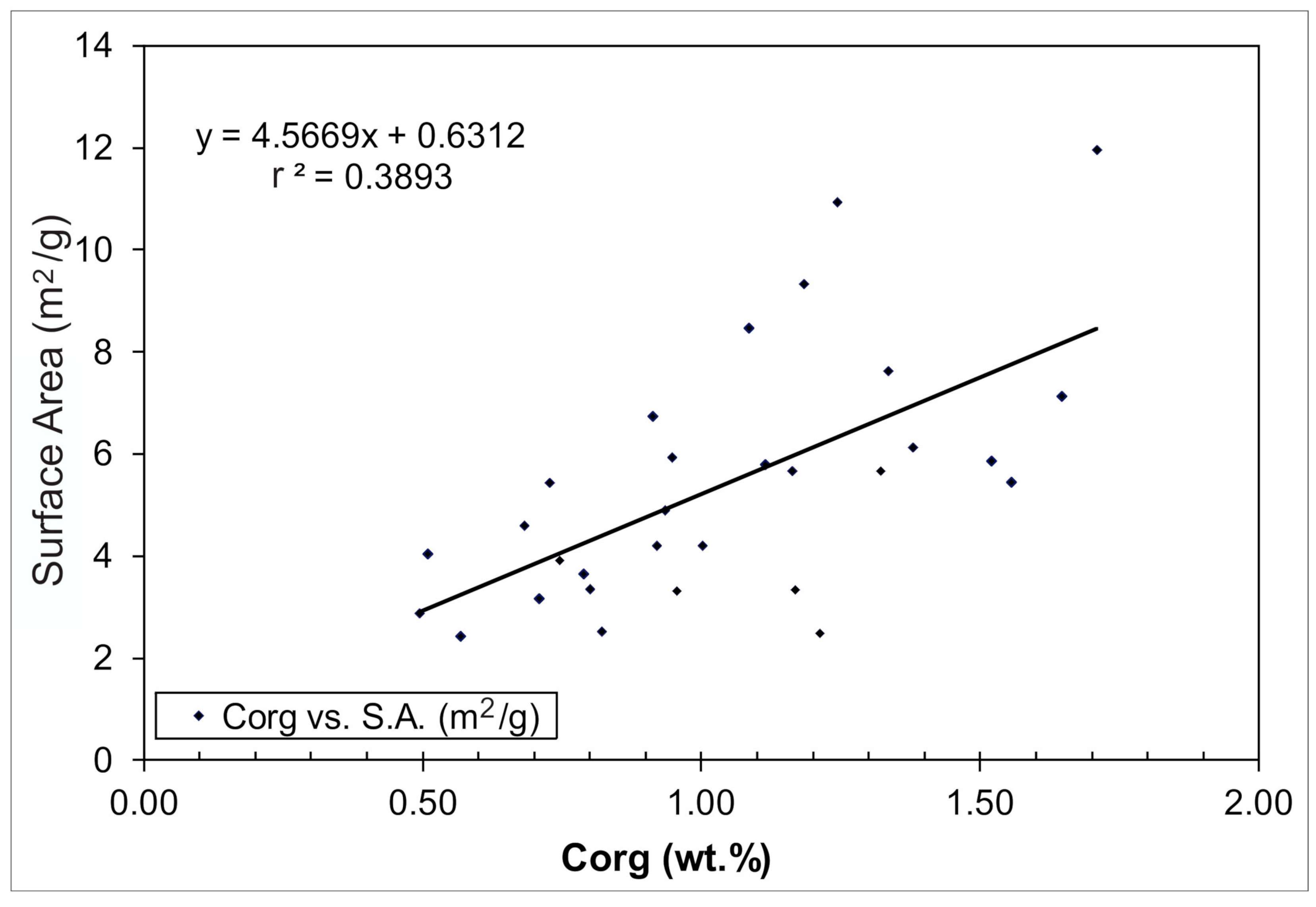
Figure 9.
Plot of Surface Area (m2/g) versus Organic Carbon (Corg) for bulk sediment samples, showing a moderate positive linear regression, r2 = 0.4.
Figure 9.
Plot of Surface Area (m2/g) versus Organic Carbon (Corg) for bulk sediment samples, showing a moderate positive linear regression, r2 = 0.4.
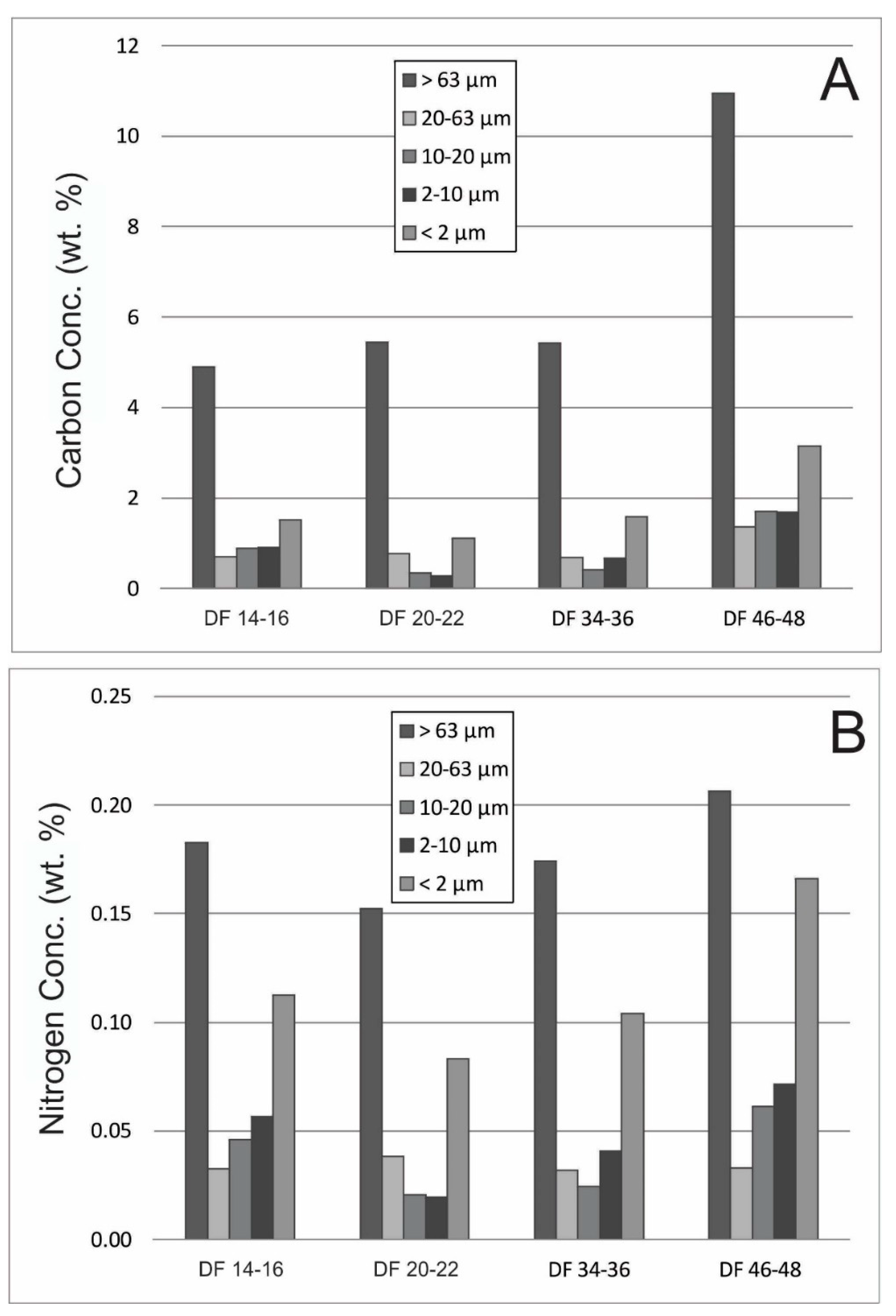
Figure 10.
Distribution of Organic Carbon (A) and Total Nitrogen (B) for four selected samples, size fractionated into five fractions: <2 μm, 2–10 μm, 10–20 μm, 20–63 μm and >63 μm.
Figure 10.
Distribution of Organic Carbon (A) and Total Nitrogen (B) for four selected samples, size fractionated into five fractions: <2 μm, 2–10 μm, 10–20 μm, 20–63 μm and >63 μm.
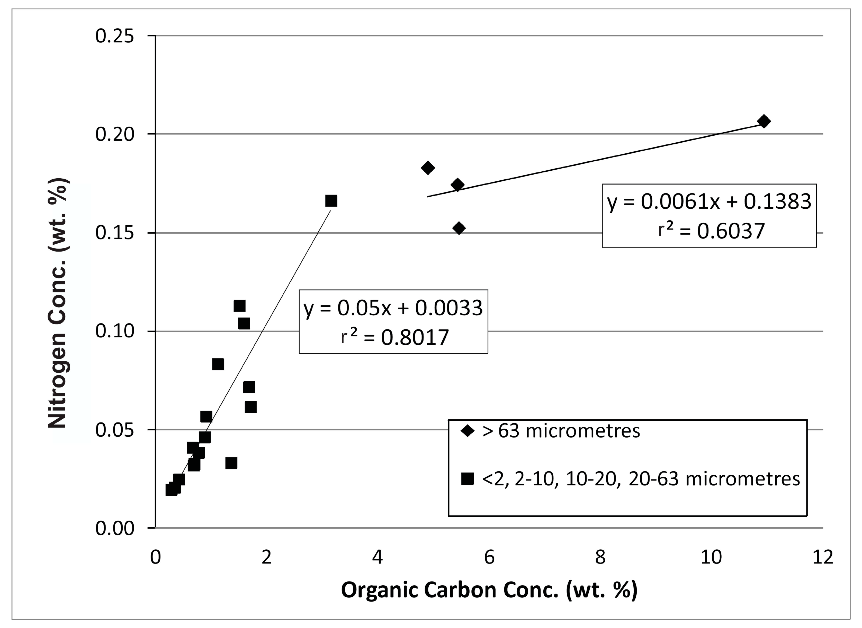
Figure 11.
Plot of Organic Carbon (Corg) versus Total Nitrogen (TN) for size fractionated samples. Note, the 63 μm fraction falls on a separate regression (r2 = 0.6) than the other four fractions (r2 = 0.8).
Figure 11.
Plot of Organic Carbon (Corg) versus Total Nitrogen (TN) for size fractionated samples. Note, the 63 μm fraction falls on a separate regression (r2 = 0.6) than the other four fractions (r2 = 0.8).
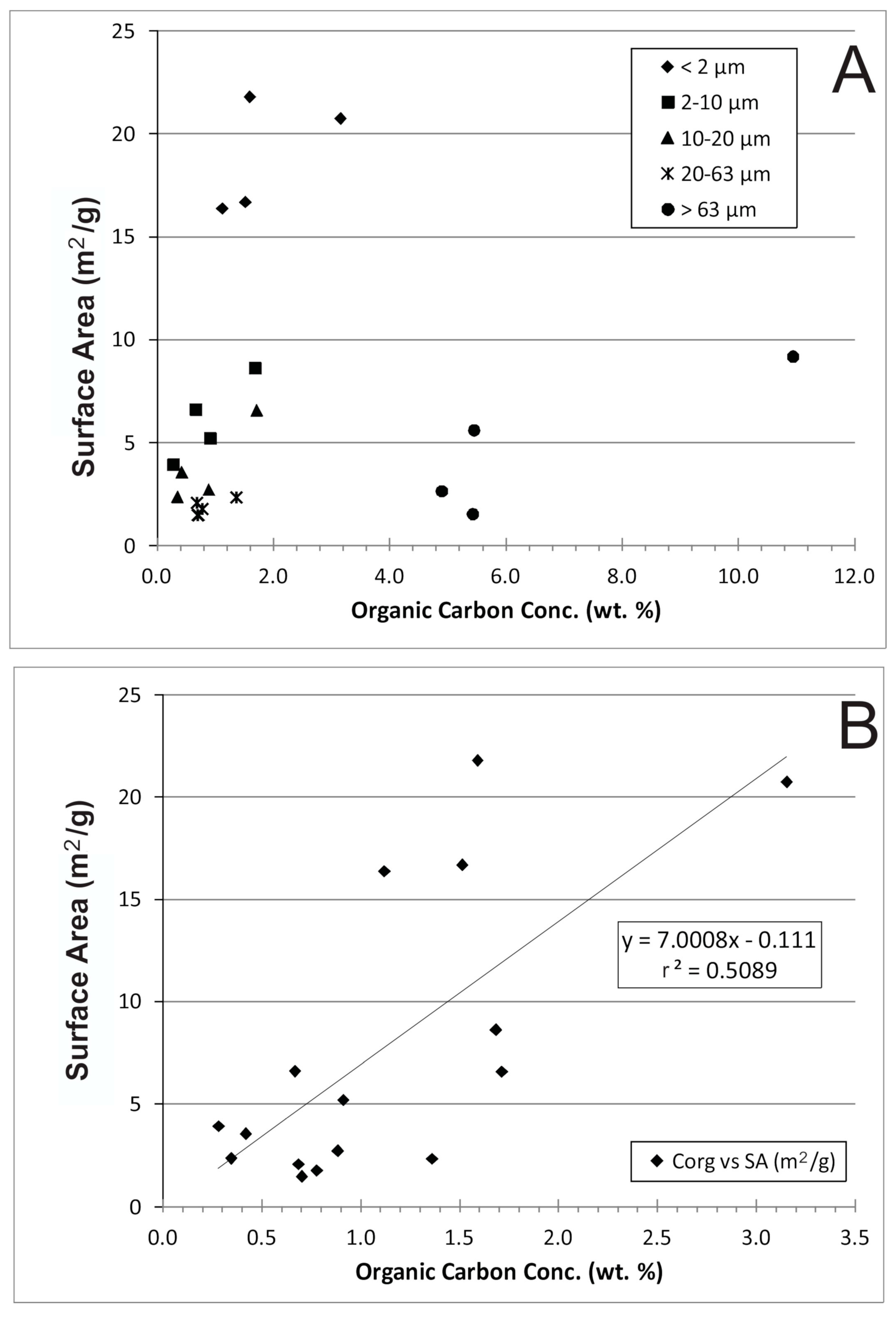
Figure 12.
(A) Plot of surface area versus organic carbon (Corg) for size fractionated samples. The >63 μm fraction plots to the right of the graph due to its high Corg content and low surface area. (B) Plot of surface area and Corg for size fractionated samples with the >63 μm fraction removed. The plot has a moderate positive correlation, r2 = 0.5.
Figure 13.
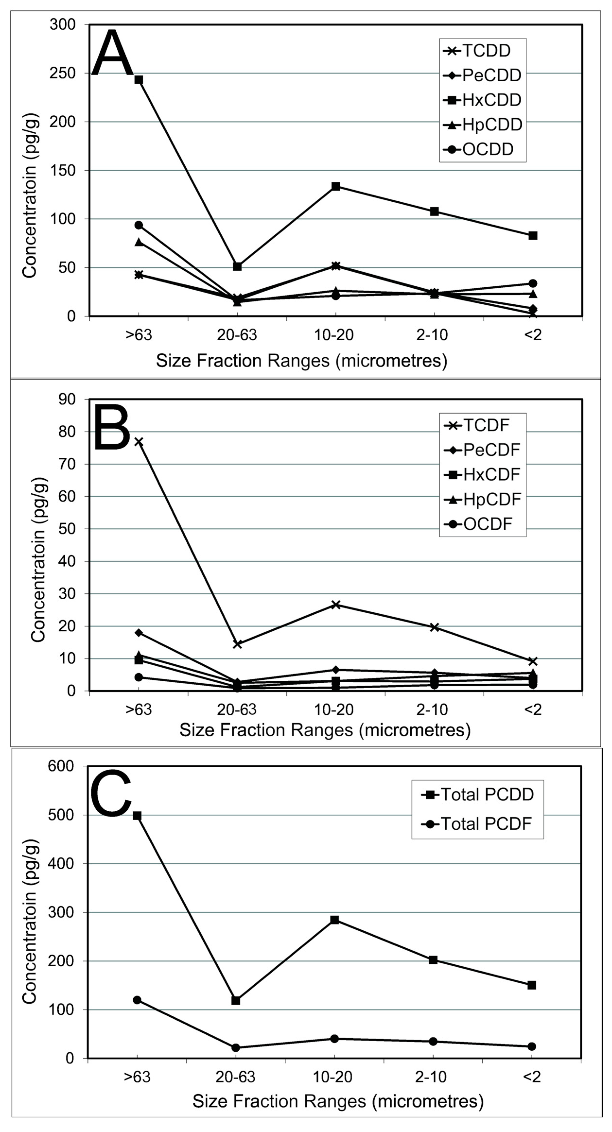
Plot showing the changes in concentration of dioxins (A), furans (B) and total homologues (C) between different size fractions at the 14–16 cm depth interval. The overall trend is of decreasing concentration with progressively finer grain size.
Figure 13.
Plot showing the changes in concentration of dioxins (A), furans (B) and total homologues (C) between different size fractions at the 14–16 cm depth interval. The overall trend is of decreasing concentration with progressively finer grain size.
Figure 14.
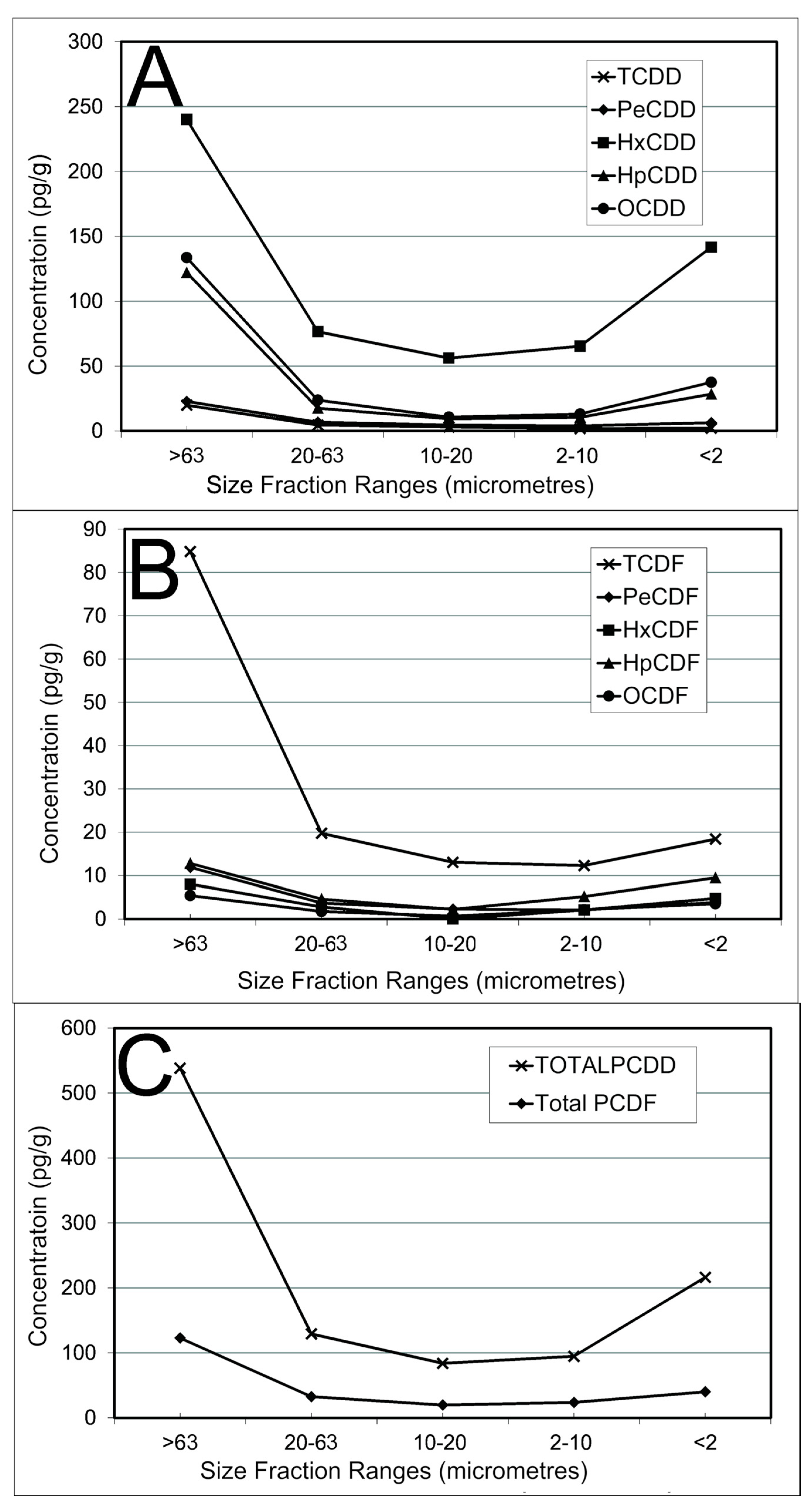
Plot showing the changes in concentration of dioxins (A), furans (B) and total homologues (C) between different size fractions at the 20–22 cm depth interval. Peak concentrations occur in the coarsest fraction. Dioxin concentration increases in the finest two size fractions, whilst furan concentration remains relatively constant throughout.
Figure 14.
Plot showing the changes in concentration of dioxins (A), furans (B) and total homologues (C) between different size fractions at the 20–22 cm depth interval. Peak concentrations occur in the coarsest fraction. Dioxin concentration increases in the finest two size fractions, whilst furan concentration remains relatively constant throughout.
Figure 15.
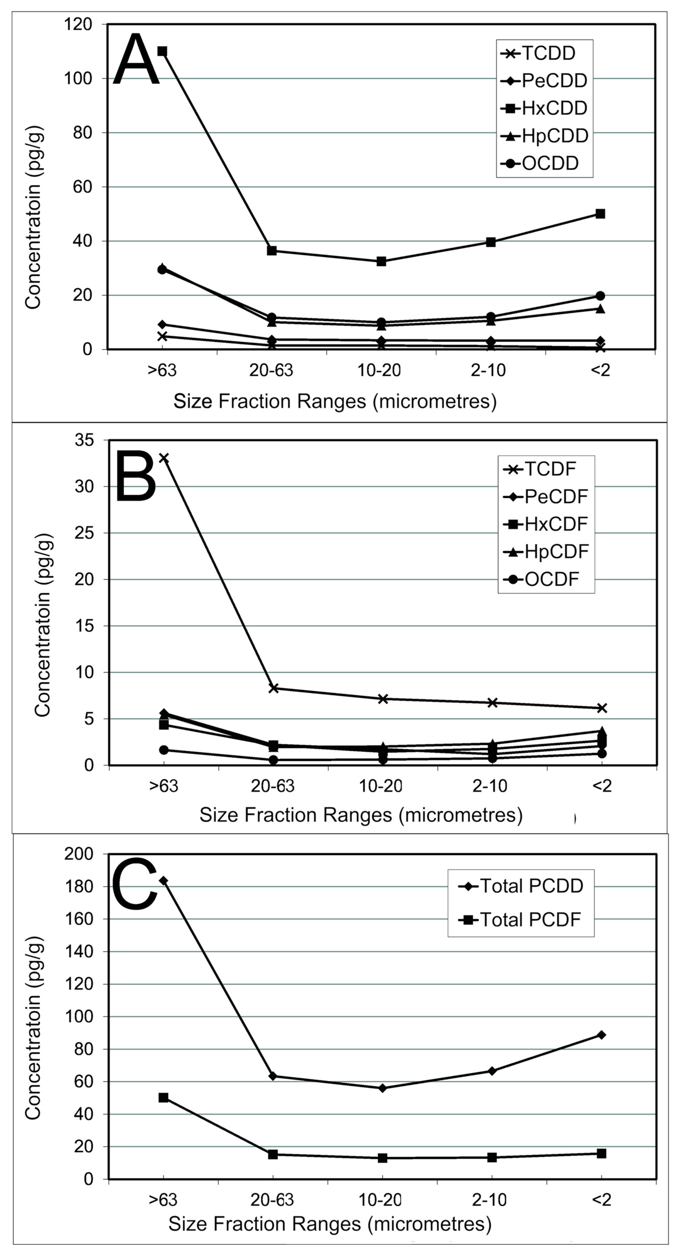
Plot showing the changes in concentration of dioxins (A), furans (B) and total homologues (C) between different size fractions at the 34–36 cm depth interval. Peak concentrations occur in the coarsest fraction. Some dioxin and furan homologues increase in concentration in the finest two size fractions, whilst other homologues show steady decrease in concentration.
Figure 15.
Plot showing the changes in concentration of dioxins (A), furans (B) and total homologues (C) between different size fractions at the 34–36 cm depth interval. Peak concentrations occur in the coarsest fraction. Some dioxin and furan homologues increase in concentration in the finest two size fractions, whilst other homologues show steady decrease in concentration.
Figure 16.
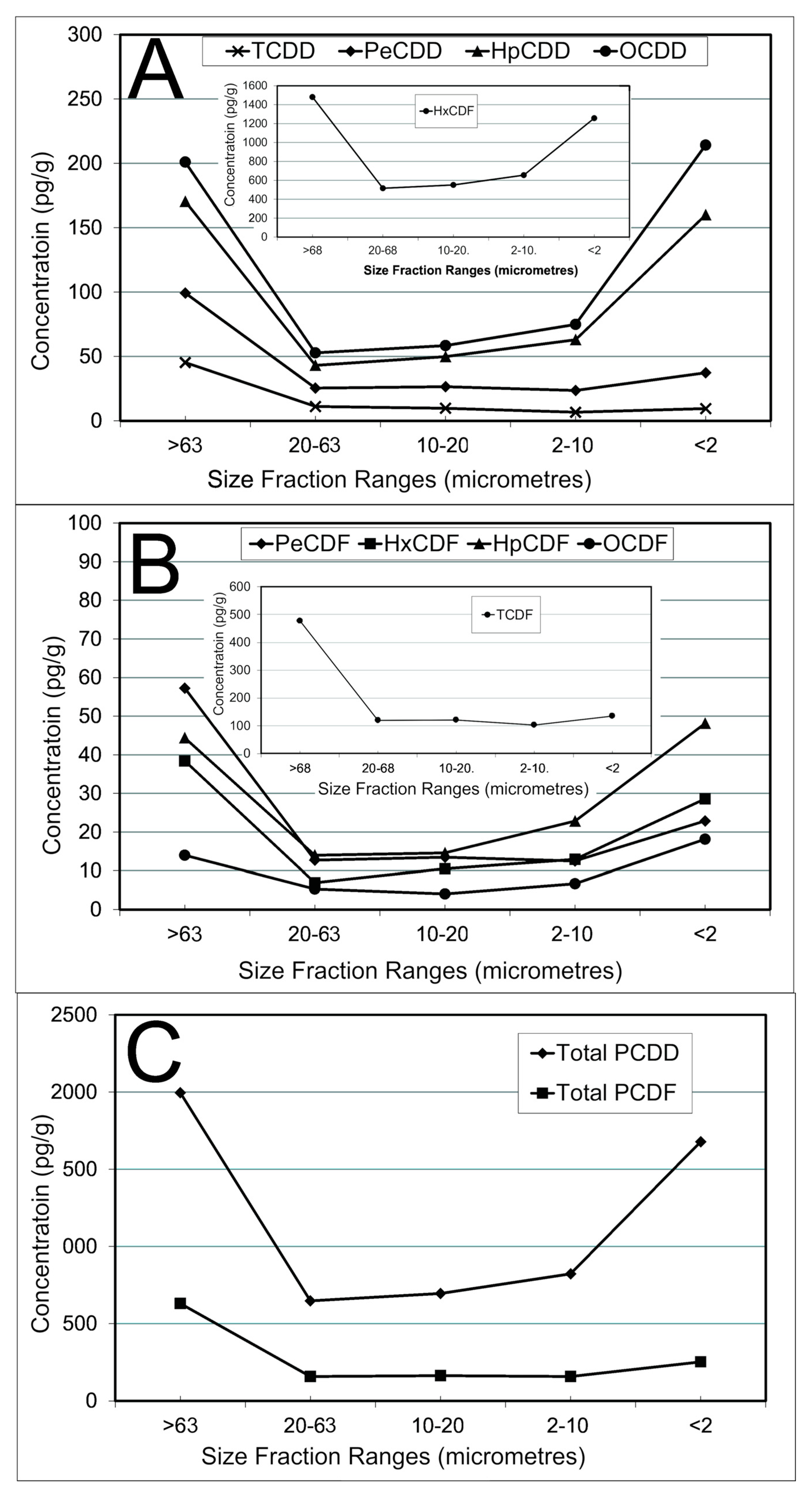
Plot showing the changes in concentration of dioxins (A), furans (B) and total homologues (C) between different size fractions at the 46–48 cm depth interval. The majority of dioxin and furan homologues show significant increase in concentration in the finest three fractions. Insets show homologues, HxCDF and TCDF, present at concentrations significantly higher than other homologues.
Figure 16.
Plot showing the changes in concentration of dioxins (A), furans (B) and total homologues (C) between different size fractions at the 46–48 cm depth interval. The majority of dioxin and furan homologues show significant increase in concentration in the finest three fractions. Insets show homologues, HxCDF and TCDF, present at concentrations significantly higher than other homologues.
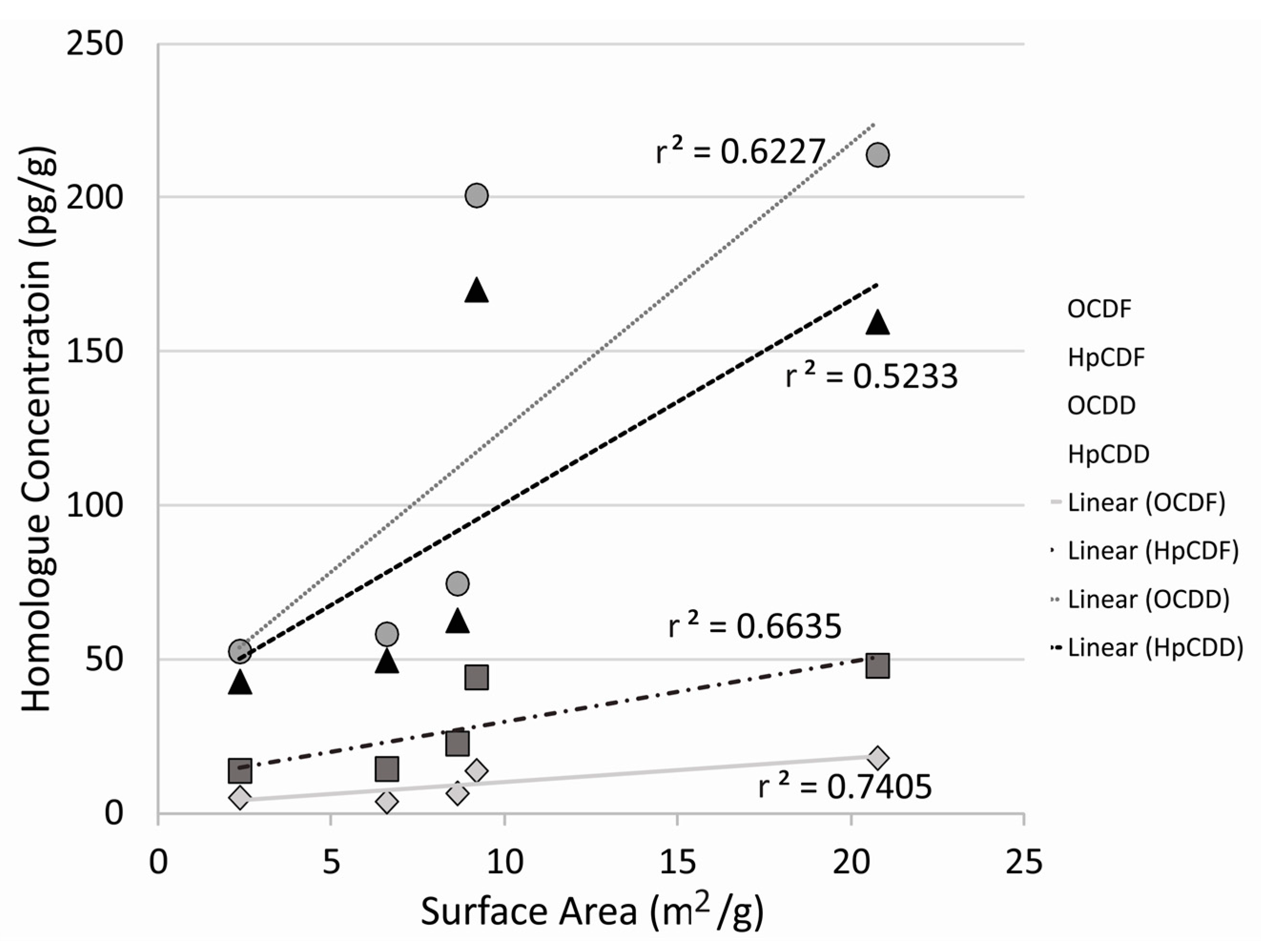
Figure 17.
Positive relationship between the concentration of four homologues and mineral surface area in sample DF 46–48. This is the only homologues that show a correlation between homologue concentration and surface area from the fractionated size samples.
Figure 17.
Positive relationship between the concentration of four homologues and mineral surface area in sample DF 46–48. This is the only homologues that show a correlation between homologue concentration and surface area from the fractionated size samples.
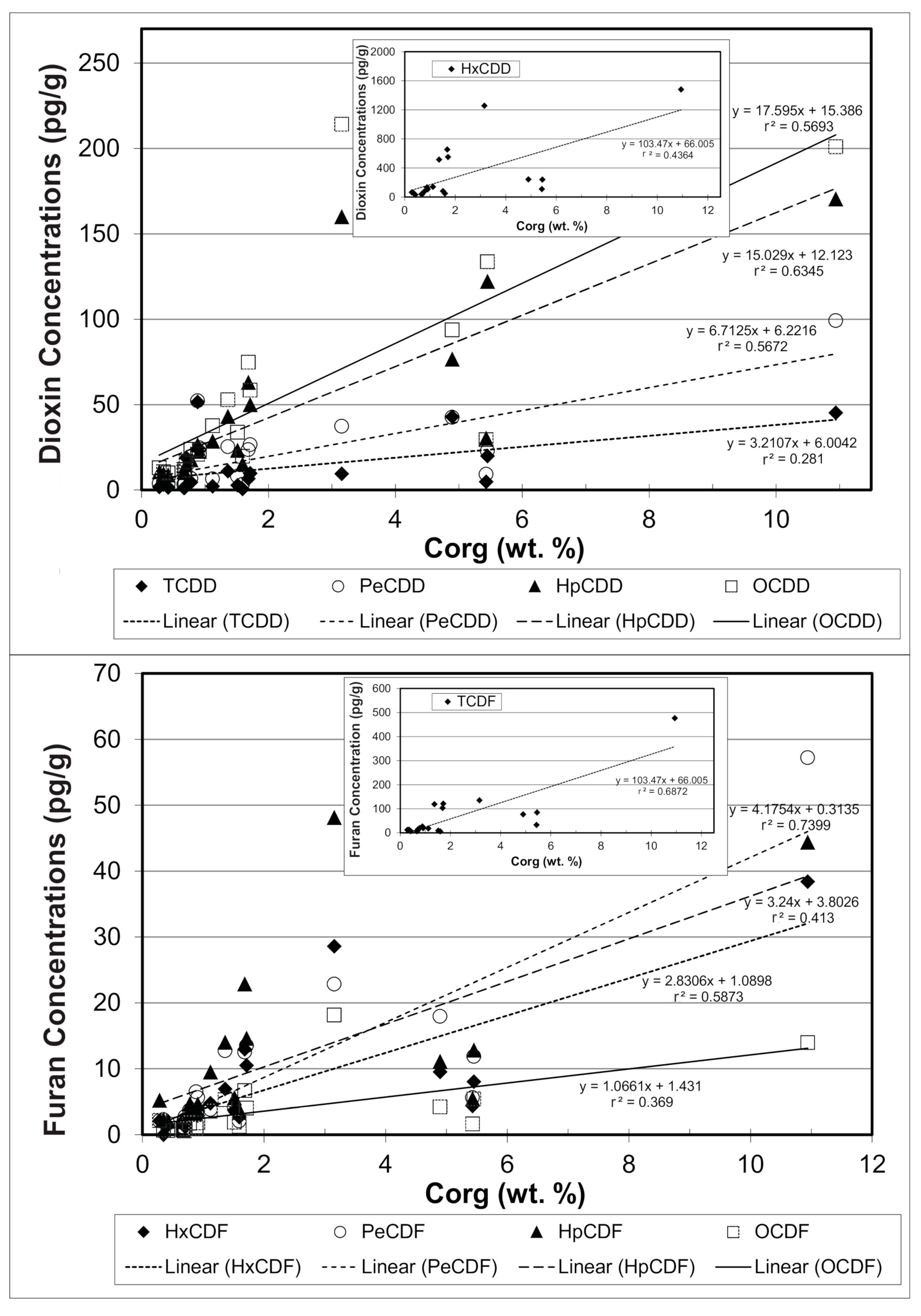
Figure 18.
Plot showing the correlation between dioxin and furan concentration and organic matter concentrations in size fractionated sediments. Inset plots are those congeners, the HxCDD and TCDF, with concentrations that are significantly higher than other congeners.
Figure 18.
Plot showing the correlation between dioxin and furan concentration and organic matter concentrations in size fractionated sediments. Inset plots are those congeners, the HxCDD and TCDF, with concentrations that are significantly higher than other congeners.
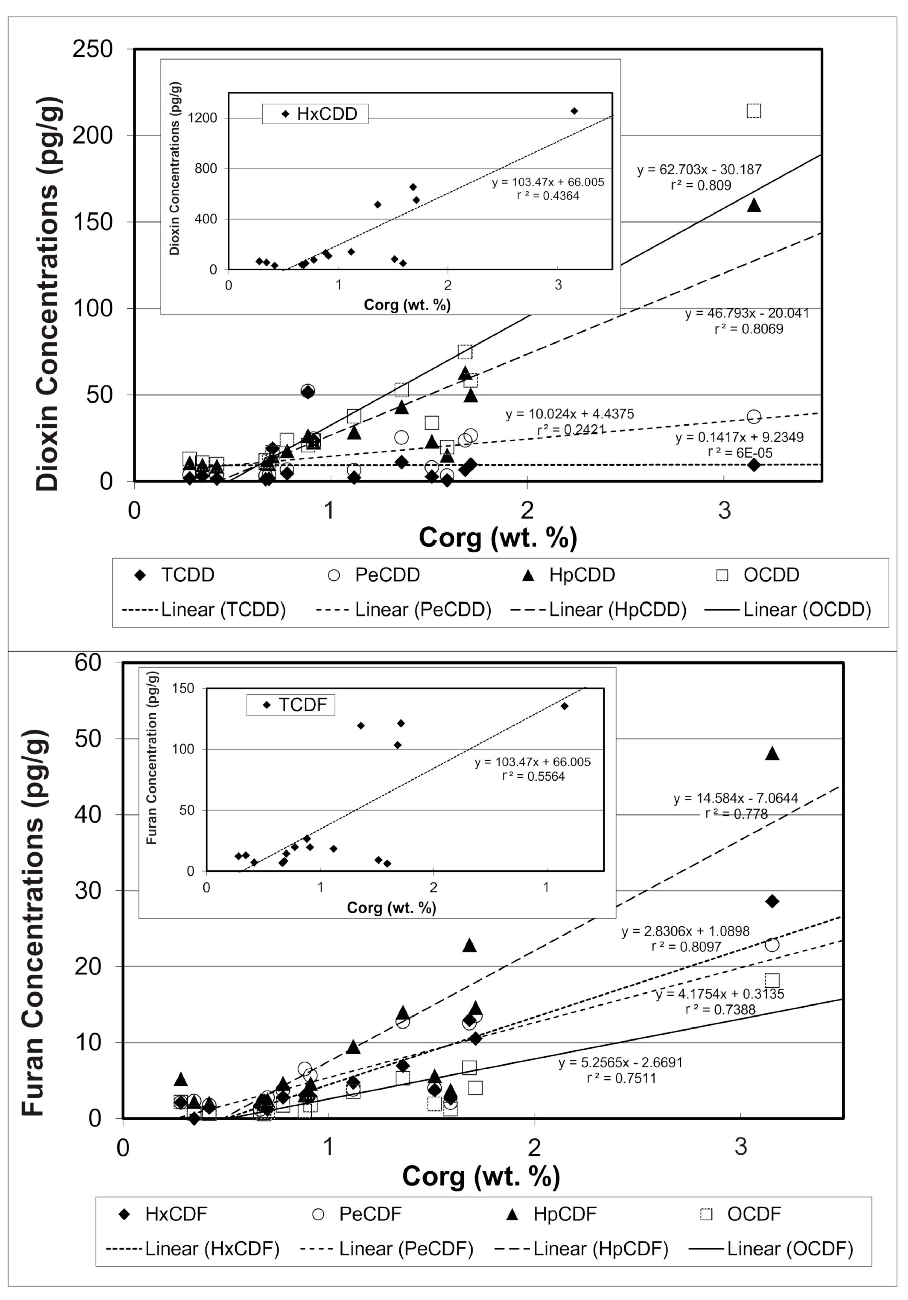
Figure 19.
Plot of dioxin and Furan concentration versus organic matter concentration with the >63 μm fraction removed. Note the increase in r2 value for HxCDD through OCDD dioxin and the decrease in r2 value for TCDD and PeCDD.
Figure 19.
Plot of dioxin and Furan concentration versus organic matter concentration with the >63 μm fraction removed. Note the increase in r2 value for HxCDD through OCDD dioxin and the decrease in r2 value for TCDD and PeCDD.
Table 1.
Composition of internal standard surrogate mixtures used to spike all samples analysed.
Table 1.
Composition of internal standard surrogate mixtures used to spike all samples analysed.
| PCDD/PCDF Surrogates Spike Volume (pg) | PCDD/PCDF Surrogates Spike Volume (pg) |
|---|
| 13C12-2,3,7,8-TCDD | 1000 |
| 13C12-1,2,3,7,8-PeCDD | 1000 |
| 13C12-1,2,3,6 7 8-HxCDD | 1000 |
| 13C12-1,2,3,4,6,7,8-HpCDD | 1000 |
| 13C12-OCDD | 2000 |
| 13C12-2,3,7,8-TCDF | 1000 |
| 13C12-1,2,3 7 8-PeCDF | 1000 |
| 13C12-1,2,3,4,7,8-HxCDF | 1000 |
| 13C12-1,2,3,4,6,7,8-HpCDF | 1000 |
Table 2.
Polychlorinated Dibenza-p-dioxins (PCDDs) and Polychlorinated Dibenza-p-furans (PCDFs) determined in each sediment sample analysed.
Table 2.
Polychlorinated Dibenza-p-dioxins (PCDDs) and Polychlorinated Dibenza-p-furans (PCDFs) determined in each sediment sample analysed.
| PCDD Congeners | PCDF Congeners |
|---|
| 2,3,7,8-TCDD | 2,3,7,8-TCDF |
| Total TCDD Homologue | Total TCDF Homologue |
| 1,2,3,7,8-PeCDD | 1,2,3,7,8-PeCDF |
| | 2,3,4,7,8-PeCDF |
| Total PeCDD Homologue | Total PeCDF Homologue |
| 1,2,3,4,7,8-HxCDD | 1,2,3,4,7,8-HxCDF |
| 1,2,3,6,7,8-HxCDD | 1,2,3,6,7,8-HxCDF |
| 1,2,3,7,8,9-HxCDD | 2,3,4,6,7,8-HxCDF |
| | 1,2,3,7,8,9-HxCDF |
| Total HxCDD Homologue | Total HxCDF Homologue |
| 1,2,3,4,6,7,8-HpCDD | 1,2,3,4,6,7,8-HpCDF |
| | 1,2,3,4,7,8,9-HpCDF |
| Total HpCDD Homologue | Total HpCDF Homologue |
| OCDD | OCDF |
Table 3.
Organic Carbon (Corg), Total Nitrogen (TN), Carbon/Nitrogen Ratio (Cor/N) and Surface Area for bulk sediment samples from the core taken adjacent to Woodfibre Pulp Mill, Howe Sound, British Columbia, subsampled every centimeter for the first ten centimeters and every two centimetres thereafter.
| Sediment Interval (cm) | Corg (wt. %) | TN (wt. %) | Corg/N | Surface Area (m2/g) |
|---|
| DF0–1 | 1.00 | 0.08 | 12.88 | 4.21 |
| DF1–2 | 1.38 | 0.10 | 13.78 | 6.13 |
| DF2–3 | 0.93 | 0.07 | 13.43 | 4.90 |
| DF3–4 | 0.57 | 0.05 | 11.99 | 2.43 |
| DF4–5 | 0.71 | 0.05 | 14.04 | 3.17 |
| DF5–6 | 0.49 | 0.04 | 12.61 | 2.88 |
| DF6–7 | 1.09 | 0.08 | 13.34 | 8.47 |
| DF7–8 | 0.96 | 0.06 | 15.25 | 3.32 |
| DF8–9 | 1.17 | 0.08 | 15.43 | 3.34 |
| DF9–10 | 1.11 | 0.09 | 12.41 | 5.80 |
| DF10–12 | 1.21 | 0.08 | 15.15 | 2.49 |
| DF12–14 | 0.82 | 0.05 | 16.03 | 2.53 |
| DF14–16 | 1.52 | 0.09 | 17.42 | 5.86 |
| DF16–18 | 1.24 | 0.09 | 13.11 | 10.94 |
| DF18–20 | 1.18 | 0.08 | 14.66 | 9.33 |
| DF20–22 | 0.91 | 0.06 | 14.08 | 6.74 |
| DF22–24 | 0.95 | 0.06 | 16.08 | 5.94 |
| DF24–26 | 0.51 | 0.04 | 11.83 | 4.05 |
| DF26–28 | 0.79 | 0.06 | 12.55 | 3.65 |
| DF28–30 | 0.73 | 0.06 | 13.16 | 5.44 |
| DF30–32 | 0.68 | 0.05 | 12.52 | 4.60 |
| DF32–34 | 0.75 | 0.05 | 14.99 | 3.92 |
| DF34–36 | 0.92 | 0.06 | 16.08 | 4.20 |
| DF36–38 | 1.32 | 0.08 | 17.43 | 5.67 |
| DF38–40 | 1.56 | 0.08 | 19.07 | 5.45 |
| DF40–42 | 0.80 | 0.05 | 16.67 | 3.36 |
| DF42–44 | 1.16 | 0.07 | 16.39 | 5.67 |
| DF44–46 | 1.33 | 0.08 | 17.24 | 7.63 |
| DF46–48 | 1.65 | 0.09 | 18.10 | 7.14 |
| DF48–50 | 1.71 | 0.07 | 23.86 | 11.96 |
| DF50–52 | 1.40 | 0.07 | 20.37 | N/A |
Table 4.
Homologue and total homologue (PCDD, PCDF) concentration (pg/g) for dioxins and furans in bulk sediment samples from selected depth intervals.
Table 4.
Homologue and total homologue (PCDD, PCDF) concentration (pg/g) for dioxins and furans in bulk sediment samples from selected depth intervals.
| Sediment Interval (cm) | TCDD | PeCDD | HxCDD | HpCDD | OCDD | Total PCDD | TCDF | PeCDF | HxCDF | HpCDF | OCDF | Total PCDF |
|---|
| DF0–1 | 3.13 | 3.84 | 15.78 | 7.29 | 11.76 | 41.8 | 3.72 | 1.48 | 1.44 | 2.32 | 1 | 9.96 |
| DF4–5 | 0.45 | 0.91 | 7.51 | 5.13 | 8.69 | 22.69 | 1.04 | 0.74 | 2.57 | 4.93 | 1.5 | 13.78 |
| DF9–10 | 1.47 | 2.52 | 17.68 | 9.58 | 16.39 | 47.64 | 3.56 | 1.37 | 1.85 | 3.3 | 1.55 | 11.63 |
| DF14–16 | 16.86 | 24.05 | 108.35 | 24.68 | 26.34 | 200.28 | 23.5 | 5.51 | 3.23 | 3.95 | 1.55 | 37.74 |
| DF20–22 | 1.52 | 3.89 | 66.75 | 14.11 | 19.52 | 105.79 | 14.19 | 2.46 | 2.42 | 4.45 | 1.78 | 25.3 |
| DF24–26 | 0.4 | 0.87 | 10.96 | 4.4 | 7.46 | 24.09 | 3.74 | 0.73 | 0.91 | 2.23 | 1.27 | 8.88 |
| DF30–32 | 0.13 | 1.47 | 14.06 | 6.32 | 8.23 | 30.21 | 2.27 | 0.89 | 0.98 | 1.26 | 0.46 | 5.86 |
| DF34–36 | 0.64 | 2.27 | 32.4 | 9.56 | 13.45 | 58.32 | 6.69 | 1.74 | 1.88 | 2.44 | 1.1 | 13.85 |
| DF40–42 | 0.13 | 0.45 | 14.58 | 4.54 | 7.31 | 27.01 | 3.42 | 0.4 | 0.65 | 1.44 | 0.49 | 6.4 |
| DF46–48 | 6.88 | 22.3 | 517.76 | 62.71 | 87.95 | 697.6 | 129.25 | 13.75 | 13.8 | 23.33 | 8.58 | 188.71 |
Table 5.
Organic Carbon (Corg), Total Nitrogen (TN), Carbon/Nitrogen Ratio (Corg/N) and Surface Area (SA) for sediment samples from selected depth intervals, size fractionated into five fractions: <2 μm, 2–10 μm, 10–20 μm, 20–63 μm and >63 μm.
Table 5.
Organic Carbon (Corg), Total Nitrogen (TN), Carbon/Nitrogen Ratio (Corg/N) and Surface Area (SA) for sediment samples from selected depth intervals, size fractionated into five fractions: <2 μm, 2–10 μm, 10–20 μm, 20–63 μm and >63 μm.
| Sediment Interval (cm) | Size Fraction (Micrometres) | Corg (wt. %) | TN (wt. %) | Corg/N | Surface Area (m2/g) |
|---|
| DF 14–16 | <2 | 1.51 | 0.11 | 13.43 | 16.68 |
| 2–10 | 0.91 | 0.06 | 16.04 | 5.20 |
| 10–20 | 0.88 | 0.05 | 19.10 | 2.72 |
| 20–63 | 0.70 | 0.03 | 21.48 | 1.49 |
| >63 | 4.90 | 0.18 | 26.77 | 2.64 |
| DF 20–22 | <2 | 1.12 | 0.08 | 13.44 | 16.37 |
| 2–10 | 0.28 | 0.02 | 14.41 | 3.92 |
| 10–20 | 0.35 | 0.02 | 16.76 | 2.37 |
| 20–63 | 0.78 | 0.04 | 20.27 | 1.78 |
| >63 | 5.45 | 0.15 | 35.78 | 5.60 |
| DF 34–36 | <2 | 1.59 | 0.10 | 15.29 | 21.80 |
| 2–10 | 0.67 | 0.04 | 16.36 | 6.61 |
| 10–20 | 0.42 | 0.03 | 17.01 | 3.55 |
| 20–63 | 0.69 | 0.03 | 21.50 | 2.08 |
| >63 | 5.43 | 0.17 | 31.14 | 1.53 |
| DF 46–48 | <2 | 3.15 | 0.17 | 19.00 | 20.75 |
| 2–10 | 1.68 | 0.07 | 23.55 | 8.62 |
| 10–20 | 1.71 | 0.06 | 27.87 | 6.58 |
| 20–63 | 1.36 | 0.03 | 41.21 | 2.34 |
| >63 | 10.94 | 0.21 | 52.99 | 9.17 |
Table 6.
Homologue and total homologue (PCDD, PCDF) concentration (pg/g) for dioxins and furans, in selected size fractionated sediment samples.
Table 6.
Homologue and total homologue (PCDD, PCDF) concentration (pg/g) for dioxins and furans, in selected size fractionated sediment samples.
| Sediment Interval (cm) | Size Fraction (Micrometres) | TCDD | PeCDD | HxCDD | HpCDD | OCDD | TOTALPCDD | TCDF | PeCDF | HxCDF | HpCDF | OCDF | Total PCDF |
|---|
| DF 14–16 | <2 | 2.75 | 8.06 | 82.87 | 23.08 | 33.77 | 150.5 | 9.11 | 3.99 | 3.72 | 5.56 | 1.91 | 24.27 |
| 2–10 | 23.8 | 24.61 | 107.8 | 22.56 | 23.56 | 202.3 | 19.61 | 5.62 | 2.9 | 4.6 | 1.78 | 34.52 |
| 10–20 | 51.51 | 52.19 | 133.8 | 26.27 | 20.9 | 284.4 | 26.59 | 6.5 | 3.05 | 3.05 | 0.98 | 40.17 |
| 20–63 | 18.94 | 16.77 | 51.11 | 14.6 | 16.6 | 118.7 | 14.38 | 2.74 | 1.19 | 2.47 | 0.86 | 21.64 |
| >63 | 42.81 | 42.58 | 243.3 | 76.49 | 93.69 | 498.9 | 76.9 | 17.94 | 9.51 | 11.09 | 4.2 | 119.65 |
| DF 20–22 | <2 | 2.17 | 6.43 | 141.7 | 28.42 | 37.55 | 216.2 | 18.4 | 3.82 | 4.75 | 9.46 | 3.54 | 39.97 |
| 2–10 | 1.82 | 3.88 | 65.4 | 10.56 | 13 | 94.66 | 12.28 | 2.11 | 2.1 | 5.11 | 2.15 | 23.81 |
| 10–20 | 3.13 | 4.54 | 56.15 | 9.37 | 10.67 | 83.87 | 13.03 | 2.28 | l.44 | 2.21 | 0.67 | 19.63 |
| 20–63 | 4.53 | 6.79 | 76.55 | 17.53 | 23.77 | 129.2 | 19.74 | 3.7 | 2.79 | 4.6 | 1.74 | 32.57 |
| >63 | 19.87 | 22.81 | 240.1 | 122.0 | 133.6 | 538.4 | 84.81 | 11.86 | 8.02 | 12.79 | 5.4 | 122.9 |
| DF 34–36 | <2 | 0.64 | 3.25 | 50.01 | 15.06 | 19.72 | 88.74 | 6.15 | 2.07 | 2.65 | 3.7 | 1.24 | 15.8 |
| 2–10 | 1.2 | 3.21 | 39.55 | 10.54 | 12.01 | 66.51 | 6.73 | 1.19 | 1.76 | 2.32 | 0.74 | 13.34 |
| 10–20 | 1.45 | 3.37 | 32.44 | 8.73 | 9.97 | 55.96 | 7.14 | 1.73 | 1.46 | 2.01 | 0.61 | 12.97 |
| 20–63 | 1.46 | 3.67 | 36.41 | 10.07 | 11.77 | 63.37 | 8.29 | 2.19 | 2.17 | 1.95 | 0.56 | 15.17 |
| >63 | 4.83 | 9.22 | 110.0 | 30.19 | 29.42 | 183.7 | 33.07 | 5.61 | 4.35 | 5.43 | 1.63 | 50.09 |
| DF 46–48 | <2 | 9.47 | 37.29 | 1257 | 159.9 | 214.1 | 1678 | 135.3 | 22.85 | 28.6 | 48.11 | 18.14 | 253.0 |
| 2–10 | 6.63 | 23.59 | 654.8 | 62.9 | 74.81 | 822.8 | 103.4 | 12.52 | 12.95 | 22.84 | 6.67 | 158.3 |
| 10–20 | 9.73 | 26.47 | 551.3 | 49.88 | 58.37 | 695.8 | 121.2 | 13.48 | 10.51 | 14.59 | 4.01 | 163.8 |
| 20–63 | 11.05 | 25.34 | 515.7 | 42.99 | 52.77 | 647.8 | 119.3 | 12.72 | 6.92 | 13.98 | 5.28 | 158.2 |
| >63 | 45.23 | 99.19 | 1480 | 170.3 | 200.9 | 1996 | 476.7 | 57.23 | 38.41 | 44.36 | 13.97 | 630.6 |
Table 7.
Regression co-efficient (r2) values for dioxin/furan/total homologue concentration (pg/g) versus surface area (m2/g). Negative values indicate a negative correlation between the two parameters. The number of size fractions indicates how many data points were used to generate the regression coefficient; r2 values using four size fractions exclude the >63 μm fraction from the calculation, r2 values using five size fractions include all the fractions.
| Sediment Interval (cm) | TCDD | PeCDD | HxCDD | HpCDD | OCDD | Total PCDD | TCDF | PeCDF | HxCDF | HpCDF | OCDF | Total PCDF |
|---|
| DF 14–16 | −0.52 | −0.39 | −0.08 | −0.05 | −0.007 | −0.13 | −0.18 | −0.09 | −0.004 | 0.002 | 0.00005 | −0.11 |
| DF 20–22 | −0.01 | 0.0004 | 0.15 | 0.01 | 0.02 | 0.05 | 0.01 | 0.004 | 0.15 | 0.29 | 0.21 | 0.01 |
| DF 34–36 | −0.03 | −0.16 | −0.03 | −0.01 | 0.008 | 0.02 | −0.18 | −0.12 | −0.004 | 0.01 | 0.06 | −0.11 |
| DF 46–48 | −0.002 | 0.02 | 0.41 | 0.52 | 0.62 | 0.4 | 0.0003 | 0.03 | 0.35 | 0.66 | 0.74 | 0.03 |


