Input-to-State Stability of a Scalar Conservation Law with Nonlocal Velocity

Abstract

In this paper, we study input-to-state stability (ISS) of an equilibrium for a scalar conservation law with nonlocal velocity and measurement error arising in a highly re-entrant manufacturing system. By using a suitable Lyapunov function, we prove sufficient and necessary conditions on ISS. We propose a numerical discretization of the scalar conservation law with nonlocal velocity and measurement error. A suitable discrete Lyapunov function is analyzed to provide ISS of a discrete equilibrium for the proposed numerical approximation. Finally, we show computational results to validate the theoretical findings.

1. Introduction

The nature of modern high-volume production is characterized by a large number of items passing through many production steps. This type of production system has fluid-like properties and has been modeled successfully by continuum models [1,2,3,4,5]. In these models, the product at different production stages and the speed of production are the quantities of interest.

Specifically, in the manufacturing system of a factory that involves a highly re-entrant system where products visit machines multiple times, such as the production of semiconductor devices, a continuum model has been introduced in [3] that is inspired by the Lighthill–Whitham traffic model [6]. The dynamics of this model is mathematically given by hyperbolic partial differential equation of the form

$${\partial }_t\rho (t,x)+\lambda \left(W\left(t\right)\right){\partial }_x\rho (t,x)=0,t\in [0,+\infty ),x\in [0,1],$$

(1)

where $\rho (t,x)$ is the product density which describes the total mass $W\left(t\right)$ at the time t and the production stage x,

$$W\left(t\right)={\int }_0^1\rho (t,x)dx,t\in (0,+\infty ).$$

(2)

Contrary to classical traffic flow models, the differential equation depends on the nonlocal quantity (2). The function $\lambda \left(W\right(t\left)\right)$ is a velocity. In production systems, it is natural to assume that the velocity function is positive and decreasing as the total mass is increasing. In the manufacturing system, the initial density of products at production stage x is taken as the initial data

$$\rho (0,x)={\rho }_0\left(x\right),x\in [0,1],$$

(3)

and the influx is used to control the system or stabilize the system at an equilibrium. Since the velocity is positive, we only require boundary conditions at $x=0$, i.e., the influx

$$\rho (t,0)\lambda \left(W\right(t\left)\right)=U\left(t\right),t\in [0,+\infty ).$$

(4)

Under suitable assumptions on $\lambda ,{\rho }_0$ and U, the existence and uniqueness of a classical solution of the Cauchy problem for the scalar conservation law Equation (1) with Equations (3) and (4) is proven in [7,8,9,10].

General stabilization problems with boundary controls have been studied in the past years in [11,12,13,14,15,16,17,18,19,20,21,22] for hyperbolic systems and recently in [7,10] for scalar conservation laws with nonlocal velocity. The focus is to derive an asymptotic stability around a given equilibrium such that solutions to the conservation laws reach the equilibrium state as time tends to infinity. Such a property is attained by an exponential stability result and presented for example in ([21], Theorem 2.3) for quasi-linear hyperbolic systems. Further references also on hyperbolic balance laws other hyperbolic systems may be found in the recent book [15].

However, when boundary controls are subjected to unknown disturbances, solutions reaching the given equilibrium point are influenced by the disturbances and a notion of asymptotic stability is required. The concept of input-to-state stability (ISS) [11,20,23] has been used to describe asymptotic stability. Concerning an asymptotic behavior of classical solutions, the Lyapunov method is used to investigate sufficient conditions to achieve an exponential stability in [16,17] for hyperbolic systems and in [7,10] for scalar conservation laws with nonlocal velocity. The Lyapunov method is also used for ISS of (local) hyperbolic systems in [11,20]. For the numerical analysis of asymptotic behavior of numerical solutions discretized by a first-order finite volume scheme, a discrete Lyapunov function is used to prove exponential stability results for hyperbolic systems in [24,25,26,27,28] and for scalar conservation laws with nonlocal velocity in [10], and ISS results for (local) hyperbolic systems could be established recently in [29,30]. Please note that the previous given references refer to ISS for hyperbolic systems. However, the theory of ISS has also been developed for other systems as for example, linear systems, time-delay equations or parabolic differential equations. A detailed review of those results is beyond the scope of this presentation and we refer the interested reader to the recent review article [31] for additional references and a review of the state-of-the-art in this field.

The previously given references refer all to ISS theory for hyperbolic problems. However, it is worth mentioning that there exists a huge amount of literature on ISS stability for problems related to other differential equations. We can not review those at this point but would like to point to some references on ISS theory for infinite-dimensional problems [32,33] and for linear [34], semi-linear [35] and nonlinear [36] parabolic system with boundary inputs. A systematic treatment of ISS using (linear) operator theory has been presented for example in [37] and non-coercive Lyapunov theory for ISS in [38,39].

Our focus in this work is hyperbolic problems. In connection with (hyperbolic) scalar conservation law with nonlocal velocity, in [10], the authors have studied global feedback stabilization of the closed-loop system in Equation (1) under the feedback law

$$U\left(t\right)-{\rho }^{*}\lambda \left({\rho }^{*}\right)=k\left(\rho (t,1)\lambda \left(W\left(t\right)\right)-{\rho }^{*}\lambda \left({\rho }^{*}\right)\right),t\in (0,+\infty ),$$

(5)

where $k\in [0,1)$ is the feedback parameter and ${\rho }^{*}\in \mathbb{R}$ is a given equilibrium. They generalize the stabilization results of [7] by using a Lyapunov function. In particular, for a given equilibrium ${\rho }^{*}=0$ and a general velocity function $\lambda \in C^1([0,+\infty );[0,+\infty ))$, the global stabilization result in $L^2$ for the closed-loop system of Equations (1), (3) and (5) is generalized to $L^p$ $(p\ge 1)$. Then, the global stabilization result in $L^2$ for the closed-loop system of Equations (1), (3) and (5) with a family of velocity functions

$$\lambda \left(s\right)=\frac{A}{B+s},s\in [0,+\infty )\mathrm{with}A>0,B>0,$$

(6)

is obtained for a given equilibrium ${\rho }^{*}>0$. By using a discrete Lyapunov function, they also established stabilization results for a discrete scalar conservation law with nonlocal velocity and using a first-order finite volume scheme.

In this paper, we study ISS for the closed-loop system of Equations (1) and (3) under the feedback law defined by

$$U\left(t\right)-{\rho }^{*}\lambda \left({\rho }^{*}\right)=k\left(\left(\rho (t,1)+d\left(t\right)\right)\lambda \left(W\left(t\right)\right)-{\rho }^{*}\lambda \left({\rho }^{*}\right)\right),t\in (0,+\infty ),$$

(7)

where $d\left(t\right)\in \mathbb{R}$ is a bounded perturbation in the measurement. In particular, we use an ISS-Lyapunov function to investigate sufficient and necessary conditions for ISS in $L^2$ for an equilibrium ${\rho }^{*}\ge 0$ and the velocity function defined by Equation (6). The numerical analysis of sufficient and necessary conditions for ISS is performed by using a discrete ISS-Lyapunov function for numerical solution obtained by a first-order finite volume scheme. Moreover, we provide numerical simulations to illustrate theoretical results for some velocity functions of type Equation (6).

The paper is organized as follows: In Section 2, we present stabilization results of ISS for a scalar conservation law with nonlocal velocity and measurement error. The numerical discretization of stabilization results of ISS for the scalar conservation law with nonlocal velocity and measurement error is presented in Section 3. Finally, in Section 4, we show numerical simulations for the scalar conservation law with nonlocal velocity and measurement error to illustrate the theoretical results.

2. Asymptotic Stability of a Scalar Conservation Law with Nonlocal Velocity and Measurement Error

We study ISS of a closed-loop system of scalar conservation laws with nonlocal velocity and measurement error of the form:

$$\left\{\begin{array}{c}{\partial }_t\rho (t,x)+\lambda \left(W\left(t\right)\right){\partial }_x\rho (t,x)=0,t\in (0,+\infty ),x\in (0,1),\hfill \\ \rho (0,x)={\rho }_0\left(x\right),x\in (0,1),\hfill \\ U\left(t\right)-{\rho }^{*}\lambda \left({\rho }^{*}\right)=k(\left(\rho (t,1)+d\left(t\right)\right)\lambda \left(W\left(t\right)\right)-{\rho }^{*}\lambda \left({\rho }^{*}\right)),t\in (0,+\infty ),\hfill \\ \rho (t,0)\lambda \left(W\right(t\left)\right)=U\left(t\right),t\in [0,+\infty ),\hfill \\ W\left(t\right)={\int }_0^1\rho (t,x)dx,t\in (0,+\infty ),\hfill \end{array}\right.$$

(8)

where $\rho (t,x)$ is the product density, $\lambda (·)\in C^1([0,+\infty ),(0,+\infty ))$ is the velocity function, $W\left(t\right)$ is total mass, $U\left(t\right)$ is the controller and $k\in [0,1)$ is a non-negative feedback parameter, ${\rho }^{*}\ge 0$ is an equilibrium solution and $d\left(t\right)\in \mathbb{R}$ is a bounded (known) perturbation in the measurement. A weak solution of the closed-loop system in Equation (8) is defined below.

Definition 1.

(Weak solution). Fix $T>0.$ A function $\rho \in C^0([0,T];L^1(0,1))$ is called a weak solution to Equation (8) if for every $s\in (0,T]$ and every $\phi \in C^1([0,s]\times [0,1])$ satisfying

$$\phi (s,x)=0,\forall x\in [0,1]\mathrm{and}\phi (t,1)=\kappa \phi (t,0),\forall t\in [0,s],$$

the following equation holds:

$$\begin{array}{cc}\hfill & {\int }_0^s{\int }_0^1\rho (t,x)\left({\partial }_t\phi (t,x)+\lambda \left(W\left(t\right)\right){\partial }_x\phi (t,x)\right)dxdt\hfill \\ \hfill & +{\int }_0^s((1-k){\rho }^{*}\lambda \left({\rho }^{*}\right)+d\left(t\right))\phi (t,0)dt+{\int }_0^1\rho (0,x)\phi (0,x)dx=0.\hfill \end{array}$$

Let $d\equiv 0$, ${\rho }^{*}\ge 0$, $p\in [1,+\infty )$ and $k\in [0,1]$ be given. Then, the existence and uniqueness of the non-negative weak solution $\rho \in C^0([0,+\infty );L^p(0,1))$ and the non-negative classical solution $\rho \in C^1([0,+\infty )\times [0,1])$ of the closed-loop system in Equation (8) are available in [7,10].

We now analyze ISS for the system Equation (8) with ${\rho }^{*}\ge 0$ in the sense of the following definitions. This is also known as global ISS. Note that ISS Lyapunov functions can be defined within a very general setting and we refer to ([31], Definition 2.11) for such a definition. In Definition (3) below, we introduce ISS-Lyapunov functions tailored to system Equation (8).

Definition 2.

(Input-to-state stability (ISS) Let $D>0.$ An equilibrium ${\rho }^{*}\ge 0$ of the closed-loop system in Equation (8) is exponential ISS in $L^2$-norm with respect to any disturbance function $d(·)\in L^{\infty }(0,\infty )$ such that ${\parallel d\parallel }_{L^{\infty }(0,\infty )}\le D$ if there exist positive constants ${\gamma }_1,{\gamma }_2,{\gamma }_3$ independent of d such that, for every initial condition ${\rho }_0\left(x\right)\in L^2(0,1)$, the $L^2$-solution to the closed-loop system in Equation (8) satisfies

$${\parallel \rho (t,·)-{\rho }^{*}\parallel }_{L^2}\le {\gamma }_2{e}^{-{\gamma }_{1}t}{\parallel {\rho }_0-{\rho }^{*}\parallel }_{L^2}+{\gamma }_3{\parallel d\left(s\right)\parallel }_{L^{\infty }(0,t)},t\in [0,+\infty ).$$

(9)

Hence, the equilibrium ${\rho }^{*}$ is ISS with respect to disturbances $d\in \mathcal{D}:=\{d(·)\in L^{\infty }(0,\infty ):\parallel d{\parallel }_{L^{\infty }}\le D\}.$

Definition 3.

(ISS-Lyapunov function). The function $\mathbf{L}:L^2(0,1)\to {\mathbb{R}}_{+}$ is said to be an ISS-Lyapunov function for the closed-loop system in Equation (8) if

(i) 

there exist positive constants ${\alpha }_1>0$ and ${\alpha }_2>0$ such that for all solutions $\rho \in C^0([0,\infty );L^2(0,1))$ and $t\in [0,+\infty )$

$${\alpha }_1\parallel \rho (t,·)-{\rho }^{*}{\parallel }_{L^2}^2\le \mathbf{L}\left(\rho (t,·)\right)\le {\alpha }_2{\parallel \rho (t,·)-{\rho }^{*}\parallel }_{L^2}^2,$$

(10)

(ii) 

there exist positive constants $\eta >0$ and $\nu >0$ such that for all solutions $\rho \in C^0([0,\infty );L^2(0,1))$ and $t\in [0,+\infty )$

$$\frac{d}{dt}\mathbf{L}\left(\rho (t,·)\right)\le -\eta \mathbf{L}\left(\rho (t,·)\right)+\nu d^2\left(t\right).$$

For a notion of differentiability of $\mathbf{L}$, we also refer for example to ([31], Section 2.2). To simplify the notation we also introduce the function

$$\mathcal{L}\left(t\right):=\mathbf{L}\left(\rho \right(t,·\left)\right),$$

(11)

where $\rho \in C^0([0,\infty );L^2(0,1))$ is the solution to Equation (8).

Theorem 1.

(ISS for ${\rho }^{*}\ge 0$). Fix any ${\rho }^{*}\ge 0$, $k\in [0,1)$, $R>0,D>0$ and any ${\rho }_0\in L^2(0,1)$ satisfying ${\rho }_0\ge 0$ a.e. in $(0,1)$. Assume further

$$\parallel {\rho }_0(·)-{\rho }^{*}{\parallel }_{L^2(0,1)}\le R.$$

(12)

Assume there exists a non-negative almost everywhere weak solution $\rho \in C^0([0,+\infty );L^2(0,1))$ to the Cauchy problem in Equation (8) where λ is given by Equation (6).

Then, the steady-state ${\rho }^{*}$ of the system in Equation (8) is exponential ISS in $L^2$-norm with respect to any disturbance function $d\in \{d(·)\in L^{\infty }(0,\infty ):\parallel d{\parallel }_{L^{\infty }}\le D\}$.

Before we begin the proof of Theorem 1, we consider the following transformation at the equilibrium ${\rho }^{*}$,

$$\begin{array}{cc}\hfill & \tilde{\rho }(t,x):=\rho (t,x)-{\rho }^{*},\tilde{W}\left(t\right):=W\left(t\right)-{\rho }^{*},\widetilde{{\rho }_0}\left(x\right):={\rho }_0\left(x\right)-{\rho }^{*},\hfill \\ \hfill & {\tilde{\lambda }}_{\tilde{W}}\left(t\right):=\lambda ({\rho }^{*}+\tilde{W}\left(t\right)),\tilde{U}\left(t\right):={\tilde{\lambda }}_{\tilde{W}}\left(t\right)\tilde{\rho }(t,0).\hfill \end{array}$$

Then, the system in Equation (8) with Equation (6) can be rewritten as follows for $t\in (0,+\infty )$:

$$\left\{\begin{array}{c}{\partial }_t\tilde{\rho }(t,x)+{\tilde{\lambda }}_{\tilde{W}}\left(t\right){\partial }_x\tilde{\rho }(t,x)=0,x\in (0,1),\hfill \\ \tilde{\rho }(0,x)={\tilde{\rho }}_0\left(x\right),x\in (0,1),\hfill \\ \tilde{U}\left(t\right)=k{\tilde{\lambda }}_{\tilde{W}}\left(t\right)\left(\tilde{\rho }(t,1)+d\left(t\right)\right)+(1-k){\rho }^{*}\left(\lambda \left({\rho }^{*}\right)-{\tilde{\lambda }}_{\tilde{W}}\left(t\right)\right),\hfill \\ {\tilde{\lambda }}_{\tilde{W}}\left(t\right):=\lambda ({\rho }^{*}+\tilde{W}\left(t\right)),\hfill \\ \tilde{W}\left(t\right)={\int }_0^1\tilde{\rho }(t,x)dx\ge -{\rho }^{*},\hfill \\ \lambda \left(s\right)=\frac{A}{B+s},\mathrm{with}A>0,B>0,s\in [0,+\infty ).\hfill \end{array}\right.$$

(13)

By using the velocity function Equation (6) in Equation (13), we have

$${\rho }^{*}\left(\lambda \left({\rho }^{*}\right)-{\tilde{\lambda }}_{\tilde{W}}\left(t\right)\right)=\theta {\tilde{\lambda }}_{\tilde{W}}\left(t\right)\tilde{W}\left(t\right),t\in [0,+\infty ),$$

(14)

where

$$\begin{array}{c}\hfill \theta :=\frac{{\rho }^{*}}{B+{\rho }^{*}}<1.\end{array}$$

For convenience, until the end of this proof, we omit the symbol “~”. Then, the system in Equation (13) with Equation (14) can be rewritten in the following form for $t\in (0,+\infty )$:

$$\left\{\begin{array}{c}{\partial }_t\rho (t,x)+{\lambda }_W\left(t\right){\partial }_x\rho (t,x)=0,x\in (0,1),\hfill \\ \rho (0,x)={\rho }_0\left(x\right),x\in (0,1),\hfill \\ U\left(t\right)=k{\lambda }_W\left(t\right)\left(\rho (t,1)+d\left(t\right)\right)+(1-k)\theta {\lambda }_W\left(t\right)W\left(t\right)\mathrm{with}\theta =\frac{{\rho }^{*}}{B+{\rho }^{*}},\hfill \\ {\lambda }_W\left(t\right):=\lambda ({\rho }^{*}+W\left(t\right)),\hfill \\ \rho (t,0){\lambda }_W\left(t\right)=U\left(t\right),\hfill \\ W\left(t\right)={\int }_0^1\rho (t,x)dx\ge -{\rho }^{*},\hfill \\ \lambda \left(s\right)=\frac{A}{B+s},\mathrm{with}A>0,B>0,s\in [0,+\infty ).\hfill \end{array}\right.$$

(15)

With the above notation, the assumption in Equation (12) of Theorem 1 reads

$$\parallel {\rho }_0{\parallel }_{L^2(0,1)}\le R.$$

(16)

Proof. 

The following proof of Theorem 1 is an extension of the proof of Theorem 3.2 in [10]. Since $C^1$-functions are dense in $L^2(0,1)$, we can analyze ISS for the system Equation (15) with non-negative weak solution $\rho \in C^0([0,+\infty );L^2(0,1))$ as follows: For $\varphi \in L^2(0,1)$, we first define a candidate ISS-Lyapunov function by

$$\begin{array}{c}\hfill \mathbf{L}\left(\varphi \right)={\int }_0^1{\varphi }^2\left(x\right)e^{-\beta x}dx+a{\left({\int }_0^1\varphi \left(x\right)dx\right)}^2.\end{array}$$

and then we have according to (11)

$$\mathcal{L}\left(t\right):=\mathbf{L}\left(\rho (t,·)\right)={\int }_0^1{\rho }^2(t,x)e^{-\beta x}dx+a{W}^2\left(t\right),\forall t\in [0,+\infty ),$$

(17)

where $\beta >0$ and $a\in \mathbb{R}$ are constants. By definition of W and Hölder inequality, we have

$$\begin{array}{c}\hfill W{\left(t\right)}^2={\left({\int }_0^1\rho (t,x)e^{-\frac{1}{2}\beta x}{e}^{\frac{1}{2}\beta x}dx\right)}^2\le {\int }_0^1{e}^{\beta x}dx{\int }_0^1{e}^{-\beta x}{\rho }^2(t,x)dx.\end{array}$$

(18)

Hence, if

$$a>-\frac{\beta }{e^{\beta }-1},$$

(19)

then $\mathcal{L}\left(t\right)>0$ for all $t\ge 0$. We will further assume from now on that $a\le 0.$ Furthermore, for $0<C_1:=C_1\left(\beta \right)=\frac{e^{\beta }-1}{\beta }$ we obtain

$$\begin{array}{c}\hfill W^2\left(t\right)\le C_1{\int }_0^1{e}^{-\beta x}{\rho }^2(t,x)dx\end{array}$$

(20)

and for $C_2:=C_2(a,\beta )=C_1+max\{a,1\}>0$ we have

$$\begin{array}{c}\hfill \mathcal{L}\left(t\right)\le C_2{\int }_0^1{e}^{-\beta x}{\rho }^2(t,x)dx.\end{array}$$

(21)

Since $a<0$ we also obtain

$$\begin{array}{c}\hfill (1+a{C}_1){\int }_0^1{e}^{-\beta x}{\rho }^2(t,x)dx\le \mathcal{L}\left(t\right).\end{array}$$

(22)

Summarizing, there exist positive constants $C_i=C_i(a,\beta )$, $i\in \{3,4\}$ such that for all $t\ge 0$

$$W^2\left(t\right)\le C_3{\int }_0^1{\rho }^2(t,x)e^{-\beta x}dx\le \mathcal{L}\left(t\right)\le C_4{\int }_0^1{\rho }^2(t,x)e^{-\beta x}dx$$

(23)

and therefore $\mathcal{L}$ is equivalent to the $L^2$-norm of $\rho .$ Note that for ${\rho }^{*}=0$ we may set $a=0$ in Equation (17). The time derivative of the candidate ISS-Lyapunov function in Equation (17) is given by:

$$\begin{array}{cc}\hfill \frac{d\mathcal{L}}{dt}\left(t\right)=& {\int }_0^{1}2\rho (t,x){\rho }_t(t,x)e^{-\beta x}dx+2aW\left(t\right)\frac{dW}{dt}\left(t\right)\hfill \\ \hfill =& -\beta {\lambda }_W\left(t\right){\int }_0^1{\rho }^2(t,x)e^{-\beta x}dx+\frac{1}{{\lambda }_W\left(t\right)}\left({\lambda }_W^2\left(t\right){\rho }^2(t,0)-{\lambda }_W^2\left(t\right){\rho }^2(t,1)e^{-\beta }\right)\hfill \\ \hfill & +2aW\left(t\right)\left({\lambda }_W\left(t\right)\rho (t,0)-{\lambda }_W\left(t\right)\rho (t,1)\right)\hfill \\ \hfill =& -\beta {\lambda }_W\left(t\right){\int }_0^1{\rho }^2(t,x)e^{-\beta x}dx+A_1\left(t\right),\hfill \end{array}$$

where $A_1\left(t\right)$ contains all contributions due to the boundary conditions. In the following we will analyze and estimate $A_1$. Note that ${\lambda }_W\left(t\right)\rho (t,0)=U\left(t\right)$ and U is given by Equation (15). More precisely, we will use the following estimate for any $ϵ>0$

$$\begin{array}{cc}\hfill 2aW\left(t\right)U\left(t\right)& =2aW\left(t\right)\left(k{\lambda }_W\left(t\right)\left(\rho (t,1)+d\left(t\right)\right)+(1-k)\theta {\lambda }_W\left(t\right)W\left(t\right)\right)\hfill \\ \hfill & \le k^2{d}^2\left(t\right){\lambda }_W\left(t\right)\frac{1}{ϵ}+ϵa^2{W}^2{\lambda }_W\left(t\right)+2aW\left(t\right)\left(k{\lambda }_W\left(t\right)\rho (t,1)+(1-k)\theta {\lambda }_W\left(t\right)W\left(t\right)\right),\hfill \\ \hfill U^2\left(t\right)& ={\left(k{\lambda }_W\left(t\right)\left(\rho (t,1)+d\left(t\right)\right)+(1-k)\theta {\lambda }_W\left(t\right)W\left(t\right)\right)}^2\hfill \\ \hfill & \le (1+ϵ){\left(k{\lambda }_W\left(t\right)\rho (t,1)+(1-k)\theta {\lambda }_W\left(t\right)W\left(t\right)\right)}^2+k^2{d}^2\left(t\right){\lambda }_W^2\left(t\right)(1+\frac{1}{ϵ}).\hfill \end{array}$$

In order to simplify the notation of the following computations, we neglect the time dependence and we define

$$\begin{array}{c}\hfill y:=y\left(t\right):={\lambda }_W\left(t\right)\rho (t,1),b_1:=b_1\left(t\right):=(1+\frac{2}{ϵ})k^2{\lambda }_W\left(t\right)d^2\left(t\right)+ϵa^2{W}^2\left(t\right){\lambda }_W\left(t\right).\end{array}$$

Then, we have

$$\begin{array}{cc}\hfill A_1\left(t\right)\le & b_1+\frac{1}{{\lambda }_W}\left((1+ϵ){(ky+(1-k)\theta {\lambda }_{W}W)}^2-y^2{e}^{-\beta }\right)+2aW((k-1)y+(1-k)\theta \lambda W)\hfill \\ \hfill =& b_1+\frac{(1+ϵ)k^2-e^{-\beta }}{{\lambda }_W}{\left(y+{\lambda }_{W}W\left(\frac{a(k-1)}{(1+ϵ)k^2-e^{-\beta }}-\frac{(k-1)k(1+ϵ)\theta }{(1+ϵ)k^2-e^{-\beta }}\right)\right)}^2\hfill \\ \hfill & +{\lambda }_W{W}^2\left({\theta }^2{(k-1)}^2(1+ϵ)-2a\theta (k-1)-\frac{{(k-1)}^2}{(1+ϵ)k^2-e^{-\beta }}{(a-k(1+ϵ)\theta )}^2\right)\hfill \\ \hfill =& b_1+\frac{(1+ϵ)k^2-e^{-\beta }}{{\lambda }_W}{\left(\dots \right)}^2\hfill \\ \hfill & -{\lambda }_W{W}^2\frac{{(k-1)}^2}{(1+ϵ)k^2-e^{-\beta }}\left(a^2-2ak(1+ϵ)\theta +k^2{(1+ϵ)}^2{\theta }^2+\frac{2a\theta ((1+ϵ)k^2-e^{-\beta })}{(k-1)}-{\theta }^2(1+ϵ)((1+ϵ)k^2-e^{-\beta })\right)\hfill \\ \hfill =& b_1+\frac{(1+ϵ)k^2-e^{-\beta }}{{\lambda }_W}{\left(\dots \right)}^2\hfill \\ \hfill & -{\lambda }_W{W}^2\frac{{(k-1)}^2}{(1+ϵ)k^2-e^{-\beta }}\left(a^2-2a\theta \frac{k(1+ϵ)-e^{-\beta }}{1-k}+{\theta }^2(1+ϵ)e^{-\beta }\right)\hfill \\ \hfill =& b_1+\frac{(1+ϵ)k^2-e^{-\beta }}{{\lambda }_W}{\left(\dots \right)}^2\hfill \\ \hfill & -{\lambda }_W{W}^2\frac{{(k-1)}^2}{(1+ϵ)k^2-e^{-\beta }}{\left(a-\theta \frac{k(1+ϵ)-e^{-\beta }}{1-k}\right)}^2\hfill \\ \hfill & -{\lambda }_W{W}^2\frac{{(k-1)}^2}{(1+ϵ)k^2-e^{-\beta }}\left({\theta }^2(1+ϵ)e^{-\beta }-{\theta }^2{\left(\frac{k(1+ϵ)-e^{-\beta }}{1-k}\right)}^2\right).\hfill \end{array}$$

Even so, it is not necessary that the proof simplifies if $ϵ$ is chosen depending on $\beta .$ We set for

$$\begin{array}{c}\hfill ϵ:=ϵ\left(\beta \right)={\beta }^2.\end{array}$$

(24)

For any fixed $0\le k<1$ and all $0<{\beta }^2<{ϵ}^{*}$ with ${ϵ}^{*}:=min\{1,\frac{1}{2}\frac{1-k}{k}\}$, we have

$$\begin{array}{c}\hfill (1+{\beta }^2)k^2<(1+{\beta }^2)k<1\end{array}$$

(25)

and hence for all $\beta <min\{\sqrt{{ϵ}^{*}},{\beta }^{*}\}$ with ${\beta }^{*}:=-ln\left((1+{ϵ}^{*})k\right)$, we have

$$\begin{array}{c}\hfill e^{-\beta }>(1+{\beta }^2)k>(1+{\beta }^2)k^2.\end{array}$$

(26)

Furthermore, consider

$$\begin{array}{c}\hfill a\left(\beta \right)=\theta \frac{k(1+{\beta }^2)-e^{-\beta }}{1-k}<0.\end{array}$$

(27)

For $\beta \to 0$, we have ${lim}_{\beta \to 0}a\left(\beta \right)=-\theta >-1$ and we have ${lim}_{\beta \to 0}\frac{\beta }{e^{\beta }-1}=1$. Hence, there exists a ${\beta }^{**}>0$ such that for all $\beta \le min\{{\beta }^{*},{\beta }^{**}\}$ and for $a\left(\beta \right)$ as given by Equation (27), the inequalities (26), (27) and (19) hold true. Using the inequality (26) and the particular choice for $a\left(\beta \right)$ and $ϵ\left(\beta \right)$, we obtain for all $\beta$ sufficiently small

$$\begin{array}{cc}\hfill A_1\left(t\right)& \le b_1\left(t\right)+{\theta }^2{\lambda }_W{W}^2\frac{{(k-1)}^2(1+{\beta }^2)e^{-\beta }-{(k(1+{\beta }^2)-e^{-\beta })}^2}{e^{-\beta }-(1+{\beta }^2)k^2}\hfill \end{array}$$

(28)

$$\begin{array}{cc}\hfill & =\left(1+\frac{2}{{\beta }^2}\right)k^2{\lambda }_W{d}^2+{\beta }^2{a}^2\left(\beta \right)W^2{\lambda }_W+{\theta }^2{\lambda }_W{W}^2{b}_2(\beta ,k),\hfill \end{array}$$

(29)

$$\begin{array}{cc}\hfill b_2(\beta ,k)& :=\frac{{(k-1)}^2(1+{\beta }^2)e^{-\beta }-{(k(1+{\beta }^2)-e^{-\beta })}^2}{e^{-\beta }-(1+{\beta }^2)k^2}.\hfill \end{array}$$

(30)

Using the estimate (20) to bound $W^2$ and using $k<1$, we obtain

$$\begin{array}{cc}\hfill A_1\left(t\right)\le & \left(1+\frac{2}{{\beta }^2}\right)k^2{\lambda }_W{d}^2+{\lambda }_W{\theta }^2\frac{e^{\beta }-1}{\beta }\left({\beta }^2\frac{a^2\left(\beta \right)}{{\theta }^2}+b_2(\beta ,k)\right){\int }_0^1{e}^{-\beta x}{\rho }^2(t,x)dx\hfill \\ \hfill \le & {\lambda }_W\left(1+\frac{2}{{\beta }^2}\right)d^2+{\lambda }_W{\theta }^2{b}_3(\beta ,k){\int }_0^1{e}^{-\beta x}{\rho }^2(t,x)dx,\hfill \\ \hfill b_3(\theta ,k):=& \frac{e^{\beta }-1}{\beta }\left({\beta }^2\frac{a^2\left(\beta \right)}{{\theta }^2}+b_2(\beta ,k)\right).\hfill \end{array}$$

An elementary computation shows that $f(\beta ,k)$ has the following properties

$$\begin{array}{c}\hfill b_3(0,k)=0 \mathrm{and} {\partial }_{\beta }{b}_3(0,k)=1.\end{array}$$

Replacing $b_3$ by a second-order Taylor expansion in $\beta$ at $\beta =0$ therefore yields the estimate

$$\begin{array}{cc}\hfill A_1\left(t\right)\le & \left(1+\frac{2}{{\beta }^2}\right){\lambda }_W{d}^2+{\theta }^2{\lambda }_W\left(\beta +O\left({\beta }^2\right)\right){\int }_0^1{e}^{-\beta x}{\rho }^2(t,x)dx.\hfill \end{array}$$

(31)

Now, we proceed with the estimate of $\frac{d}{dt}\mathcal{L}\left(t\right)$ as

$$\begin{array}{cc}\hfill \frac{d}{dt}\mathcal{L}\left(t\right)\le & -\beta {\lambda }_W\left(t\right){\int }_0^1{e}^{-\beta x}{\rho }^2(t,x)dx\left(1-{\theta }^2+O\left(\beta \right)\right)+\left(1+\frac{2}{{\beta }^2}\right){\lambda }_W\left(t\right)d^2\left(t\right).\hfill \end{array}$$

(32)

Since $\theta <1$ there exists $0<\overline{\beta }<min\{{\beta }^{*},{\beta }^{**}\}$ sufficiently small, such that

$$\begin{array}{c}\hfill 0<1-{\theta }^2+O\left(\beta \right).\end{array}$$

(33)

Using the estimate (22) there is a constant $0<\eta :=\eta (k,{\rho }^{*})$, we obtain

$$\begin{array}{cc}\hfill \frac{d}{dt}\mathcal{L}\left(t\right)\le & -\eta {\lambda }_W\left(t\right)\mathcal{L}\left(t\right)+\left(1+\frac{2}{{\overline{\beta }}^2}\right){\lambda }_W\left(t\right)d^2\left(t\right).\hfill \end{array}$$

(34)

By definition, we have that $0\le {\lambda }_W\left(t\right)$. Next, we show that ${\lambda }_W\left(t\right)$ is bounded from below by a positive constant. This requires to obtain an upper bound on $W\left(t\right).$ The previous inequality (34) yields the following bound on $W^2\left(t\right)$ for $C_5:=C_5\left(\overline{\beta }\right)=\frac{C_1}{(1+a)C_1}$ and for $C_6:=C_6\left(\overline{\beta }\right)=\left(1+\frac{2}{{\overline{\beta }}^2}\right):$

$$\begin{array}{cc}\hfill \frac{1}{C_5}{W}^2\left(t\right)\le & \mathcal{L}\left(t\right)\le e^{-\eta {\int }_0^t{\lambda }_W\left(s\right)ds}\mathcal{L}\left(0\right)+{\int }_0^t{C}_6{\lambda }_W\left(s\right)d^2\left(s\right)e^{-\eta {\int }_s^t{\lambda }_W\left(r\right)dr}\hfill \end{array}$$

(35)

$$\begin{array}{cc}\hfill \le & \mathcal{L}\left(0\right)+\frac{C_6}{\eta }{\parallel d\left(t\right)\parallel }_{L^{\infty }(0,t)}\left(1-e^{-\eta {\int }_0^t{\lambda }_W\left(s\right)ds}\right).\hfill \end{array}$$

(36)

By assumption $\parallel {\rho }_0{\parallel }^2\le R^2$. By definition we have $-{\rho }^{*}\le W\left(t\right)$ and therefore

$$\begin{array}{c}\hfill -{\rho }^{*}\le W\left(t\right)\le \sqrt{C_5{R}^2+\frac{C_5{C}_6}{\eta }{\parallel d(·)\parallel }_{L^{\infty }(0,t)}}.\end{array}$$

(37)

Due to the definition of ${\lambda }_W$, it is uniformly bounded from above by ${\sigma }_1:=\frac{A}{B}$. Furthermore, we have that $W\left(t\right)$ is bounded from above due to Equation (37) and since d is bounded. Hence, ${\lambda }_W$ is bounded from below by ${\sigma }_2={\sigma }_2{(\parallel d\parallel }_{L^{\infty }(0,\infty )},R,\overline{\beta })$. Note that the $L^{\infty }$ norm of the disturbances are uniformly bounded by the constant $D.$ This yields that for all $t\ge 0$

$$\begin{array}{c}\hfill {\sigma }_1\ge {\lambda }_W\left(t\right)\ge {\sigma }_2.\end{array}$$

(38)

Using the previous estimate for ${\lambda }_W$ in Equation (34) yields the assertion. The decay rate ${\eta }^{*}$ of the Lyapunov function is ${\eta }^{*}=\eta {\sigma }_2$ and $\nu ={\sigma }_1{C}_6.$ □

Some remarks are in order.

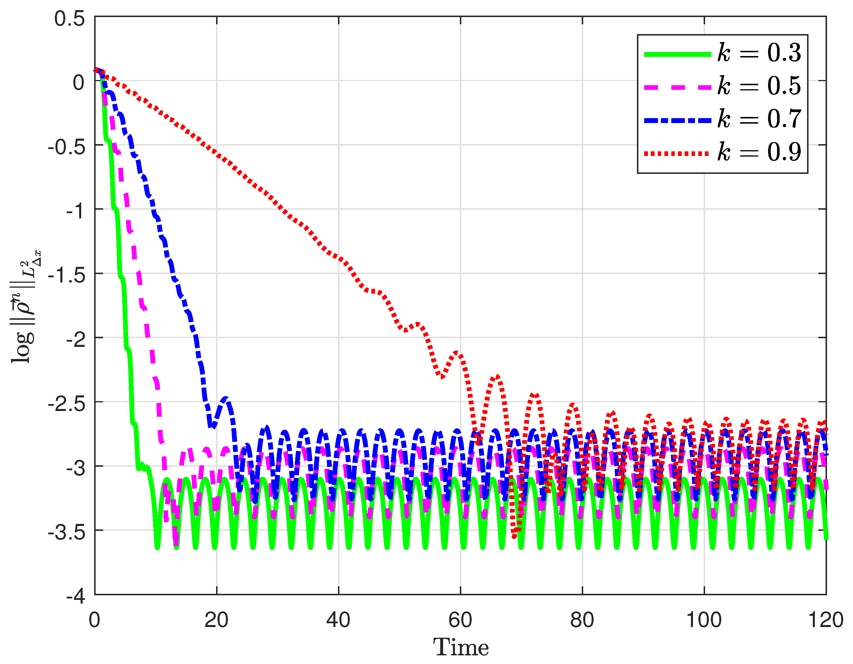
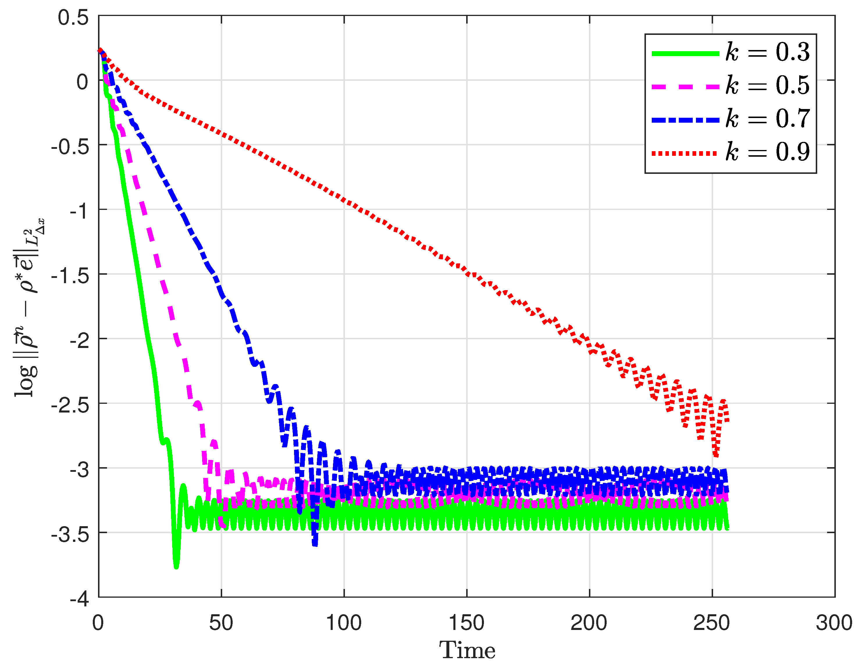
Remark 1.

Note that the rate $\eta =\eta ({\rho }^{*},k)$ as a function of k tends to zero as k tends to one, this can be seen for example in Equation (26) defining the upper bound for $\overline{\beta }.$ Similarly, if $\theta \to 1$, i.e., ${\rho }^{*}\to \infty$, we observe that $\eta \to 0$ due to Equation (33).

The bound on $W\left(t\right)$ is required to obtain the exponential decay. Therefore, the final rate depends on the constant R and we refer to Equation (37) and following for its detailed dependence. Note that in the case ${\rho }^{*}=0$ we may set $a=0$ and therefore no bound on W is necessary.

Further, the result holds true for any solution $\rho \in C^0([0,\infty );L^2(0,1))$ and hence uniqueness of solutions is not required. Regarding existence of solutions, it might be possible to extend recent results [40,41,42]. However, so far existence results in the case $d\equiv 0$ exist [10].

Note that the decay rate η will be dependent on the bound of the disturbance as well as on R, but will be uniform with respect to ${\rho }_0$ provided that ${\rho }_0$ fulfills (12).

In ([7], Lemma 3.5) it has been shown that in the case $d\equiv 0$ and ${\rho }^{*}=0$ exponential stability does not hold if $k>1.$

For ${\rho }^{*}=0$, Theorem 1 holds true for any velocity function $\lambda (·)\in C^1([0,+\infty ),(0,+\infty ))$. This case is similar to a problem studied in [10]. Therein, a detailed discussion of the case $d\equiv 0$ has been presented and we refer in particular to ([10], Theorem 3.1).

3. Numerical Study of Asymptotic Stability of a Scalar Conservation Law with Nonlocal Velocity and Measurement Error

In the following section, we extend the result to a proper discretization of the continuous dynamics. The following results are based on similar estimates as in the previous section and it is a minor extension of the proof presented in ([10], Section 4.2). In order to not repeat the estimates obtained in [10], we will use a similar notation and mostly report on the changes in estimates due to the additional disturbance $d.$ As seen in the previous proof in Equation (24), it is possible to chose $ϵ={\beta }^2$ and we will do so in the following proof directly. This simplifies the notation and reduces the technicality of the computations.

As in ([10], Section 4.2) we introduce a first-order Upwind discretization of the closed-loop system in Equation (8). To this end we divide the spatial domain $[0,1]$ using an equidistant grid with cell width $\Delta x$ and $J\in \mathbb{N}$ cells such that $\Delta xJ=1.$ The cell centers are denoted by $x_j=(j-\frac{1}{2})\Delta x,j\in \{1,\dots ,J\}$ and, the boundary of the domain are $x_0$ and $x_J$, respectively. Moreover, we discretize $W\left(t\right)$ by

$$W^n=\Delta x\sum _{j=1}^J{\rho }_j^n,n\in \{1,2,\dots \},$$

(39)

with the point wise values of the solution ${\rho }_j^n=\rho (t^n,x_j)$. Further, we define the discrete values ${\lambda }^n$ by

$${\lambda }^n:=\lambda \left(W^n\right)=\frac{A}{B+W^n},A>0,B>0,$$

(40)

where $t^n=n\Delta t,n\in \{0,1,\dots \}$ denotes the discrete time such that the time step size $\Delta t$ satisfies a stability condition due to Courant–Friedrichs–Lewy condition (CFL). This condition states that $\Delta t$ is chosen such that

$$0<r^n:=\frac{{\lambda }^n\Delta t}{\Delta x}\le 1,\forall n\in \{0,1,\dots \}.$$

(41)

Since ${\lambda }^n\le \frac{A}{B}$ for all $n\ge 0$, we can choose a possibly small but fixed $\Delta t$ such that the previous condition (41) holds true for all n with fixed $\Delta t$ and $\Delta x.$ This choice allows to take a uniform grid in time. As in the continuous case we have ${\rho }^{*}>0.$ For the given initial values ${\overrightarrow{\rho }}^0={({\rho }_0^0,{\rho }_1^0,\dots ,{\rho }_J^0)}^{\top }$ with ${\rho }_j^0\ge 0$, $j\in \{0,\dots ,J\}$, we employ a first–order finite volume scheme, given by the explicit Upwind method, to discretize the system in Equation (8).

$$\left\{\begin{array}{cc}{\rho }_j^{n+1}=\left(1-r^n\right){\rho }_j^n+r^n{\rho }_{j-1}^n,\hfill & j\in \{1,\dots ,J\},n\in \{0,1,\dots \},\hfill \\ {\rho }_0^{n+1}=k{\rho }_J^{n+1}+(1-k)\frac{{\rho }^{*}\lambda \left({\rho }^{*}\right)}{{\lambda }^{n+1}}+k{d}^{n+1},\hfill & n\in \{0,1,\dots \}.\hfill \end{array}\right.$$

(42)

We now define discrete version of ISS and ISS-Lyapunov function as follows:

Definition 4.

(Discrete ISS). Let $D>0.$ An equilibrium ${\rho }^{*}\ge 0$ of the discrete closed-loop system in Equation (42) is ISS in $L^2$-norm with respect to discrete disturbances $d^n\le D$, $n\in \{1,2,\dots \}$ if there exist positive real constants ${\gamma }_1>0$, ${\gamma }_2>0$ and ${\gamma }_3>0$ such that, for every initial condition ${\rho }_j^0$, $j\in \{1,\dots ,J\}$, the solution ${\rho }_j^n$, $j\in \{1,\dots ,J\}$, $n\in \{0,1,\dots \}$ to the discrete closed-loop system in Equation (42) satisfies

$$\parallel {\overrightarrow{\rho }}^n-{\rho }^{*}{\parallel }_{L_{\Delta x}^2}\le {\gamma }_2{e}^{-{\gamma }_1{t}^n}{\parallel {\overrightarrow{\rho }}^0\parallel }_{L_{\Delta x}^2}+{\gamma }_3\underset{0\le s<n}{max}\left(|d^s|\right),n\in \{1,2,\dots \},$$

(43)

where ${\overrightarrow{\rho }}^n={({\rho }_j^n)}_{j=1}^J$ and

$$\parallel {\overrightarrow{\rho }}^n{\parallel }_{{\ell }^2}^2:=\Delta x\sum _{j=1}^J{\left({\rho }_j^n\right)}^2,n\in \{0,1,\dots \}.$$

Definition 5.

(Discrete ISS-Lyapunov function). A function $\mathbf{L}:{\mathbb{R}}^J\to {\mathbb{R}}_0^{+}$ is said to be a discrete ISS-Lyapunov function for the discrete closed-loop system in Equation (42) if

(i)

there exist positive constants ${\alpha }_1>0$ and ${\alpha }_2>0$ such that for all $n\in \{0,1,\dots \}$

$${\alpha }_1\parallel {\overrightarrow{\rho }}^n-{\rho }^{*}{\parallel }_{{\ell }^2}^2\le \mathbf{L}\left({\overrightarrow{\rho }}^n\right)\le {\alpha }_2{\parallel {\overrightarrow{\rho }}^n-{\rho }^{*}\parallel }_{{\ell }^2}^2,$$

(44)

(ii)

there exist positive constants $\eta >0$ and $\nu >0$ such that for all $n\in \{0,1,\dots \}$

$$\frac{\mathbf{L}({\overrightarrow{\rho }}^{n+1})-\mathbf{L}({\overrightarrow{\rho }}^n)}{\Delta t}\le -\eta \mathbf{L}({\overrightarrow{\rho }}^n)+\nu {\left(d^n\right)}^2.$$

To simplify the notation later on we will define the sequence of discrete values ${\mathcal{L}}^n$ by

$${\mathcal{L}}^n:=\mathbf{L}({\overrightarrow{\rho }}^n),n\in \{0,1,\dots \}$$

(45)

and where ${\overrightarrow{\rho }}^n$ are given as solution to the system in (42).

Theorem 2.

(Discrete ISS for ${\rho }^{*}\ge 0$) Assume that the CFL condition in Equation (41) holds. Let $D>0$. For every ${\rho }^{*}\ge 0$, every $k\in [0,1)$, every $R>0$ and for every initial data ${\overrightarrow{\rho }}^0={({\rho }_0^0,{\rho }_1^0,\dots ,{\rho }_J^0)}^{\top }$ with ${\rho }_j^0\ge 0$, $j\in \{1,\dots ,J\}$ and

$$\parallel {\overrightarrow{\rho }}^0-{\rho }^{*}\overrightarrow{e}{\parallel }_{{\ell }^2}\le R,$$

(46)

where $\overrightarrow{e}=\stackrel{J+1}{\overbrace{{(1,\dots ,1)}^{\top }}}$, the solution ${\overrightarrow{\rho }}^n={({\rho }_0^n,{\rho }_1^n,\dots ,{\rho }_J^n)}^{\top }$ to the system in Equation (42) satisfies ${\rho }_j^n\ge 0$, $j\in \{0,\dots ,J\}$, $n\in \{0,1,\dots \}$ and the steady-state ${\rho }^{*}$ of the discrete system in Equation (42) is ISS in $L^2$-norm with respect any discrete disturbance function $d^n$, $n\in \{1,2,\dots \}$ such that $d^n\le D.$

In order to analyze the ISS of the discrete system in Equation (42) by the discrete Lyapunov method, we use the following transformation

$${\tilde{\rho }}_j^n={\rho }_j^n-{\rho }^{*},{\tilde{W}}^n=\Delta x\sum _{j=1}^J{\tilde{\rho }}_j^n,{\tilde{\lambda }}_{\tilde{W}}^n=\lambda \left({\rho }^{*}+{\tilde{W}}^n\right),{\tilde{r}}^n=\frac{\Delta t}{\Delta x}{\tilde{\lambda }}_{\tilde{W}}^n,n\in \{0,1,\dots \}.$$

(47)

For simplicity, we omit the symbol “~” in Equation (47) and discretize the system in Equation (15) as follows

$$\left\{\begin{array}{c}{\rho }_j^{n+1}=\left(1-r^n\right){\rho }_j^n+r^n{\rho }_{j-1}^n,j\in \{1,\dots ,J\},n\in \{0,1,\dots \},\hfill \\ {\rho }_0^{n+1}=k{\rho }_J^{n+1}+(1-k)\theta W^{n+1}+k{d}^{n+1}\mathrm{with}\theta =\frac{{\rho }^{*}}{B+{\rho }^{*}},n\in \{0,1,\dots \},\hfill \\ r^n=\frac{\Delta t}{\Delta x}{\lambda }_W^n,n\in \{0,1,\dots \},\hfill \\ {\lambda }_W^n=\lambda \left({\rho }^{*}+W^n\right),n\in \{0,1,\dots \},\hfill \\ W^n=\Delta x\sum _{j=1}^J{\rho }_j^n\ge -{\rho }^{*},n\in \{0,1,\dots \},\hfill \\ \lambda \left(s\right)=\frac{A}{B+s},s\ge 0.\hfill \end{array}\right.$$

(48)

Thus, the assumption in Equation (46) in Theorem 2 is now expressed as

$$\parallel {\overrightarrow{\rho }}^0{\parallel }_{{\ell }^2}\le R.$$

(49)

Note that the proof of Theorem 2 is an extension of the proof of Theorem 4.2 in [10]. Thus, some details of the proof can be found in [10] and we will point to the corresponding estimates in order to reduce the technicality of the proof.

Proof. 

As in the continuous case the proof simplifies if ${\rho }^{*}=0.$ Therefore, we consider in the forthcoming proof only the more interesting case

$$\begin{array}{c}\hfill {\rho }^{*}>0.\end{array}$$

(50)

Since the initial data ${\rho }_j^0\ge 0$, $j\in \{0,\dots ,J\}$, by the discrete system in Equation (48) and the CFL condition in Equation (41), we have ${\rho }_j^n\ge 0$, $j\in \{0,\dots ,J\}$, $n\in \{0,1,\dots \}$.

Consider the following candidate stretchy="false" (17) for any $\overrightarrow{\varphi }\in {\mathbb{R}}^J$

$$\mathbf{L}(\overrightarrow{\varphi })=\Delta x\sum _{j=1}^J{\left({\varphi }_j\right)}^2{e}^{-\beta x_j}+a{\left(\Delta x\sum _{j=1}^J{\varphi }_j\right)}^2.$$

where $\beta >0$. In particular, we set a

$$\begin{array}{cc}\hfill a=& \theta \frac{k-e^{-\beta }}{1-k}<0\hfill \end{array}$$

(51)

and since $\theta <1$ there exists ${\beta }^{*}$ sufficiently small such that $0>a>-\frac{\beta }{e^{\beta }-1}$, see ([10], (3.25), (3.26)).

According to (45), the values of $\mathbf{L}$ at the solution ${\overrightarrow{\rho }}^n$ at time $t^n$ for $n\ge 0$ are given by

$$\begin{array}{cc}\hfill {\mathcal{L}}^n=& \parallel {\overrightarrow{\rho }}^n{\parallel }_{\beta }^2+a{\left(W^n\right)}^2,\hfill \end{array}$$

(52)

$$\begin{array}{cc}\hfill \parallel {\overrightarrow{\rho }}^n{\parallel }_{\beta }^2:=& \Delta x\sum _{j=1}^J{\left({\rho }_j^n\right)}^2{e}^{-\beta x_j}.\hfill \end{array}$$

(53)

For fixed $k\in [0,1)$, we assume as in [10] there exists a ${\beta }^{**}$ such that for $0<\beta <{\beta }^{**}$

$$\begin{array}{c}\hfill exp(-\beta )>k>k^2 \mathrm{and} \beta <1-k,\end{array}$$

(54)

holds true and that

$$\begin{array}{c}\hfill 0<\Delta x<1.\end{array}$$

(55)

As a first step, we prove that ${\mathcal{L}}^n$ is equivalent to $\parallel {\overrightarrow{\rho }}^n{\parallel }_{\beta }^2.$ This part does not dependent on the boundary condition ${\rho }_0^{n+1}$ and is therefore analogous to [10]. In particular, due to estimate ([10], (4.32), (4.34)) we have for all $n\ge 1$

$$\begin{array}{cc}\hfill {\left(W^n\right)}^2\le & {\Delta x}^2\sum _{j=1}^J{\left({\rho }_j^n\right)}^2{e}^{-\beta x_j}\sum _{j=1}^J{e}^{\beta x_j}\le \frac{\Delta x(e^{\beta }-1)}{1-e^{-\beta \Delta x}}{\parallel {\overrightarrow{\rho }}^n\parallel }_{\beta }^2\hfill \end{array}$$

(56)

$$\begin{array}{cc}\hfill \le & {\left(1+\beta \right)}^2\parallel {\overrightarrow{\rho }}^n{\parallel }_{\beta }^2\le (1+3\beta ){\parallel {\overrightarrow{\rho }}^n\parallel }_{\beta }^2.\hfill \end{array}$$

(57)

Due to the bounds on a, we obtain the estimate ([10], (4.38)) for all $n\ge 0$

$$\begin{array}{cc}\hfill \parallel {\overrightarrow{\rho }}^n{\parallel }_{\beta }^2\ge {\mathcal{L}}^n\ge & \parallel {\overrightarrow{\rho }}^n{\parallel }_{\beta }^2\left(1+\theta \frac{k-e^{-\beta }}{1-k}\frac{\Delta x(e^{\beta }-1)}{1-e^{-\beta \Delta x}}\right)\hfill \end{array}$$

(58)

$$\begin{array}{cc}\hfill \ge & (1-\theta (1+3\beta ))\parallel {\overrightarrow{\rho }}^n{\parallel }_{\beta }^2\ge \frac{1-\theta }{2}{\parallel {\overrightarrow{\rho }}^n\parallel }_{\beta }^2,\hfill \end{array}$$

(59)

where the last inequality is true provided that

$$\begin{array}{c}\hfill 0<\beta \le min\{1,{\beta }^{*},{\beta }^{**},\frac{1-\theta }{6\theta }\}.\end{array}$$

(60)

Furthermore, the discrete weighted norm is equivalent to the ${\ell }^2$-norm as in ([10], (4.39)) for all $n\ge 0$

$$\begin{array}{c}\hfill e^{-\beta }\parallel {\overrightarrow{\rho }}^n{\parallel }_{{\ell }^2}^2\le \parallel {\overrightarrow{\rho }}^n{\parallel }_{\beta }^2\le {\parallel {\overrightarrow{\rho }}^n\parallel }_{{\ell }^2}.\end{array}$$

(61)

As a second step, we estimate a finite difference approximation to the temporal derivative of $\mathcal{L}.$

$$\begin{array}{cc}\hfill \frac{{\mathcal{L}}^{n+1}-{\mathcal{L}}^n}{\Delta t}& =\frac{\Delta x}{\Delta t}\sum _{j=1}^J\left[{\left({\rho }_j^{n+1}\right)}^2-{\left({\rho }_j^n\right)}^2\right]e^{-\beta x_j}\hfill \end{array}$$

(62)

$$\begin{array}{cc}\hfill & +\frac{a{\left(\Delta x\right)}^2}{\Delta t}\left[{\left(\sum _{j=1}^J{\rho }_j^{n+1}\right)}^2-{\left(\sum _{j=1}^J{\rho }_j^n\right)}^2\right].\hfill \end{array}$$

(63)

Precisely, as in [10], we use the discrete scheme (48), the CFL condition (41) that ensures $0<r^j\le 1$ and the convexity $z\to z^2$ to estimate for all $i=1,\dots ,J$ and $n\ge 0$

$$\begin{array}{c}\hfill {\left({\rho }_i^{n+1}\right)}^2={[(1-r^n){\rho }_i^n+r^n{\rho }_{i-1}^n]}^2\le (1-r^n){\left({\rho }_i^n\right)}^2+r^n{({\rho }_j^n)}^2.\end{array}$$

(64)

Then, we obtain the discrete counterpart to the integration by parts formula

$$\begin{array}{cc}\hfill \frac{{\mathcal{L}}^{n+1}-{\mathcal{L}}^n}{\Delta t}\le & {\lambda }_W^n\left(\sum _{j=1}^J{\left({\rho }_{j-1}^n\right)}^2{e}^{-\beta x_{j-1}}{e}^{-\beta \Delta x}-\sum _{j=1}^J{({\rho }_j^n)}^2{e}^{-\beta x_j}\right)\hfill \end{array}$$

(65)

$$\begin{array}{cc}\hfill +& \frac{a{(\Delta x)}^2}{\Delta t}\left({\left(\sum _{j=1}^J{\rho }_j^n-r^n{\rho }_J^n+r^n{\rho }_0^n\right)}^2-{\left(\sum _{j=1}^J{\rho }_j^n\right)}^2\right)\hfill \end{array}$$

(66)

$$\begin{array}{cc}\hfill =& {\lambda }_W^n{e}^{-\beta \Delta x}\left(\frac{1}{\Delta x}{\parallel {\overrightarrow{\rho }}^n\parallel }_{\beta }^2-e^{-\beta }{\left({\rho }_J^n\right)}^2+{\left({\rho }_0^n\right)}^2\right)-\frac{{\lambda }_W^n}{\Delta x}{\parallel {\overrightarrow{\rho }}^n\parallel }_{\beta }^2\hfill \end{array}$$

(67)

$$\begin{array}{cc}\hfill +& \frac{a}{\Delta t}\left({\left(W^n-r^n\Delta x{\rho }_J^n+r^n\Delta x{\rho }_0^n\right)}^2-{\left(W^n\right)}^2\right)\hfill \end{array}$$

(68)

$$\begin{array}{cc}\hfill =& \frac{e^{-\beta \Delta x}-1}{\Delta x}{\lambda }_W^n{\parallel \overrightarrow{\rho }\parallel }_{\beta }^2+A_1^n.\hfill \end{array}$$

(69)

Here, the last line is as in ([10], (4.29)) except that the boundary term ${\rho }_0^n$ that is part of $A_1^n$ includes now the disturbance $d^n.$ We split the boundary condition at $x=0$ as

$$\begin{array}{c}\hfill {\rho }_0^n={\overline{\rho }}_0^n+k{d}^n,{\overline{\rho }}_0^n:=k{\rho }_J^n+(1-k)\theta W^n\end{array}$$

(70)

and obtain

$$\begin{array}{cc}\hfill A_1^n=& {\lambda }_W^n{e}^{-\beta \Delta x}\left({\left({\overline{\rho }}_0^n+k{d}^n\right)}^2-e^{-\beta }{\left({\rho }_J^n\right)}^2\right)\hfill \end{array}$$

(71)

$$\begin{array}{cc}\hfill & +a{\lambda }_W^n\left(r^n\Delta x{\left({\overline{\rho }}_0^n+k{d}^n-{\rho }_J^n\right)}^2+2\left({\overline{\rho }}_0^n+k{d}^n-{\rho }_J^n\right)W^n\right).\hfill \end{array}$$

(72)

As in the continuous case, we estimate

$$\begin{array}{c}\hfill {\left({\overline{\rho }}_0^n+k{d}^n\right)}^2\le (1+{\beta }^2){\left({\overline{\rho }}_0^n\right)}^2+(1+\frac{1}{{\beta }^2}){\left(k{d}^n\right)}^2\end{array}$$

(73)

and similarly for the term $2k{d}^n{W}^n$ and ${\left({\overline{\rho }}_0^n+k{d}^n-{\rho }_J^n\right)}^2,$ respectively. Hence, we obtain

$$\begin{array}{cc}\hfill A_1^n\le & A_2^n+A_3^n+A_4^n,\hfill \\ \hfill A_2^n:=& {\lambda }_W^n{e}^{-\beta \Delta x}\left({\left({\overline{\rho }}_0^n\right)}^2-e^{-\beta }{\left({\rho }_J^n\right)}^2\right)+a{\lambda }_W^n\left(r^n\Delta x{\left({\overline{\rho }}_0^n-{\rho }_J^n\right)}^2+2\left({\overline{\rho }}_0^n-{\rho }_J^n\right)W^n\right),\hfill \\ \hfill A_3^n:=& {\beta }^2{\lambda }_W^n{e}^{-\beta \Delta x}{\left({\overline{\rho }}_0^n\right)}^2+{\beta }^2\parallel a\parallel {\lambda }_W^n{r}^n\Delta x{\left({\overline{\rho }}_0^n-{\rho }_J^n\right)}^2+{\beta }^2{\lambda }_W^n{\left(W^n\right)}^2,\hfill \\ \hfill A_4^n:=& {\lambda }_W^n{e}^{-\beta \Delta x}(1+\frac{1}{{\beta }^2}){\left(k{d}^n\right)}^2+\parallel a\parallel {\lambda }_W^n{r}^n\Delta x(1+\frac{1}{{\beta }^2}){\left(k{d}^n\right)}^2+\frac{1}{{\beta }^2}\parallel a\parallel {\lambda }_W^n{\left(k{d}^n\right)}^2.\hfill \end{array}$$

Next, we estimate $A_3^n$ and $A_4^n$. Here, we use that a defined by (51), ${\lambda }_W^n$, are bounded by

$$\begin{array}{c}\hfill \parallel a\parallel \le \frac{\beta }{e^{\beta }-1}\le 1,{\lambda }_W^n\le \frac{A}{B}, \mathrm{and} r^n\le 1,\end{array}$$

respectively, and that $r^n,\Delta x$ and $\theta$ are all bounded by one. Additionally, we have a bound on ${\left(W^n\right)}^2$ due to (56) and $\beta \le 1$ by (60) such that

$$\begin{array}{c}\hfill {\left({\overline{\rho }}_0^n\right)}^2\le 2{\left({\rho }_J^n\right)}^2+2{\left(W^n\right)}^2\le \left(2+2(1+3)\right)\parallel {\overrightarrow{\rho }}^n{\parallel }_{\beta }^2, \mathrm{and} {\left({\overline{\rho }}_0^n-{\rho }_J^n\right)}^2\le 22{\parallel {\overrightarrow{\rho }}^n\parallel }_{\beta }^2.\end{array}$$

Hence, there exists a constant $C>0$ such that $A_3^n$ and $A_4^n$ are estimated by

$$\begin{array}{c}\hfill A_3^n\le C{\beta }^2{\lambda }_W^n{\parallel {\overrightarrow{\rho }}^n\parallel }_{\beta }^2 \mathrm{and} A_4^n\le (1+\frac{3}{{\beta }^2}){\lambda }_W^n{\left(d^n\right)}^2.\end{array}$$

(74)

A crucial estimate is now performed on $A_2^n.$ Due to the previous estimates as well as due to Equation (70) we have that $A_2^n$ coincides with ([10], $A_2$) and hence we may use the same estimates ([10], (4.31), (4.34)) to obtain

$$\begin{array}{cc}\hfill A_2^n\le & {\lambda }_W^n{\theta }^2{\left(W^n\right)}^2\left((k-e^{-\beta })(2-e^{\beta \Delta x})+e^{-\beta \Delta x}(1-k)\right)\hfill \\ \hfill \le & {\lambda }_W^n{\theta }^2(1+3\beta ){\parallel {\overrightarrow{\rho }}^n\parallel }_{\beta }^2\left((k-e^{-\beta })(2-e^{\beta \Delta x})+e^{-\beta \Delta x}(1-k)\right)\hfill \\ \hfill \le & {\lambda }_W^n{\theta }^2(1+3\beta ){\parallel {\overrightarrow{\rho }}^n\parallel }_{\beta }^2\beta .\hfill \end{array}$$

The previous estimates allow to estimate the discrete temporal derivative of $\mathcal{L}$ in Equation (65) for $n\ge 0:$

$$\begin{array}{cc}\hfill \frac{{\mathcal{L}}^{n+1}-{\mathcal{L}}^n}{\Delta t}\le & \frac{e^{-\beta \Delta x}-1}{\Delta x}{\lambda }_W^n{\parallel \overrightarrow{\rho }\parallel }_{\beta }^2+A_2^n+A_3^n+A_4^n\hfill \\ \hfill \le & \left((-\beta +\frac{\Delta x}{2}{\beta }^2)+{\theta }^2(\beta +3{\beta }^2)+C{\beta }^2\right){\lambda }_W^n{\parallel \overrightarrow{\rho }\parallel }_{\beta }^2+(1+\frac{3}{{\beta }^2}){\lambda }_W^n{\left(d^n\right)}^2,\hfill \\ \hfill \le & -\beta \left(1-\frac{\beta }{2}-{\theta }^2(1+3\beta )-C\beta \right){\lambda }_W^n{\parallel \overrightarrow{\rho }\parallel }_{\beta }^2+(1+\frac{3}{{\beta }^2}){\lambda }_W^n{\left(d^n\right)}^2,\hfill \\ \hfill \le & -\beta \frac{1-{\theta }^2}{2}{\lambda }_W^n{\parallel {\overrightarrow{\rho }}^n\parallel }_{\beta }^2+(1+\frac{3}{{\beta }^2}){\lambda }_W^n{\left(d^n\right)}^2.\hfill \end{array}$$

The last inequality holds true provided that $0<\beta$ is sufficiently small such that (60) and

$$\begin{array}{c}\hfill \beta \le \frac{1-{\theta }^2}{7+2C}.\end{array}$$

(75)

hold true.

Finally, it remains to show that ${\lambda }_W^n$ is bounded from below by a strictly positive number. This is equivalent to show that $W^n$ is bounded from above and similar to the continuous analysis. Note that due to $\parallel {\overrightarrow{\rho }}^n{\parallel }_{\beta }^2\ge {\mathcal{L}}^n$ and therefore

$$\begin{array}{c}\hfill \frac{{\mathcal{L}}^{n+1}-{\mathcal{L}}^n}{\Delta t}\le -b_1{\lambda }_W^n{\mathcal{L}}^n+b_2{\left(d^n\right)}^2,\end{array}$$

(76)

$$\begin{array}{c}\hfill b_1:=b_1\left(\beta \right)=\beta \frac{1-{\theta }^2}{2},b_2:=b_2\left(\beta \right):=1+\frac{3}{{\beta }^2}.\end{array}$$

(77)

Solving recursively (76), we obtain with ${\prod }_{r=n+1}^n(·)=1$

$$\begin{array}{cc}\hfill {\mathcal{L}}^{n+1}\le & \prod _{m=0}^n(1-\Delta t{b}_1{\lambda }_W^m){\mathcal{L}}^0+b_2\Delta t\sum _{m=0}^n{\lambda }_W^m{\left(d^m\right)}^2\prod _{r=m+1}^n(1-b_1\Delta t{\lambda }_W^r)\hfill \end{array}$$

(78)

$$\begin{array}{cc}\hfill \le & exp\left(-b_1\Delta t\sum _{m=0}^n{\lambda }_W^m\right){\mathcal{L}}^0+\underset{0\le s\le n}{max}{\left(d^s\right)}^2{b}_2\Delta t\sum _{m=0}^n{\lambda }_W^m\prod _{r=m+1}^n(1-b_1\Delta t{\lambda }_W^r).\hfill \end{array}$$

(79)

The following equalities show that the last term of the previous sum can be bounded independent of ${\lambda }_W^n:$

$$\begin{array}{cc}\hfill -\frac{1}{b_1\Delta t}\sum _{m=0}^n-b_1\Delta t{\lambda }_W^m& \prod _{r=m+1}^n(1-b_1\Delta t{\lambda }_W^r)\hfill \end{array}$$

(80)

$$\begin{array}{cc}\hfill =& -\frac{1}{b_1\Delta t}\sum _{m=0}^n(1-b_1\Delta t{\lambda }_W^m-1)\prod _{r=m+1}^n(1-b_1\Delta t{\lambda }_W^r)\hfill \end{array}$$

(81)

$$\begin{array}{cc}\hfill =& -\frac{1}{b_1\Delta t}\sum _{m=0}^n\left(\prod _{r=m}^n(1-b_1\Delta t{\lambda }_W^r)-\prod _{r=m+1}^n(1-b_1\Delta t{\lambda }_W^r)\right)\hfill \end{array}$$

(82)

$$\begin{array}{cc}\hfill =& -\frac{1}{b_1\Delta t}\prod _{r=0}^n(1-b_1\Delta t{\lambda }_W^r)-1\hfill \end{array}$$

(83)

$$\begin{array}{cc}\hfill =& \frac{1}{b_1\Delta t}\left(1-\prod _{r=0}^n(1-b_1\Delta t{\lambda }_W^r)\right).\hfill \end{array}$$

(84)

Note that since $b_1<1$ and $\Delta t$ fulfills the CFL condition (41) we have that for all $n\ge 0,$

$$\begin{array}{c}\hfill b_1\Delta t{\lambda }_W^n\le b_1\Delta x\le 1\end{array}$$

and therefore $1-b_1\Delta t{\lambda }_W^r$ is non–negative. stretchy="false" $-{\rho }^{*}\le W^n$ and due to (59) and (60), we have

$$\begin{array}{c}\hfill {\left(W^n\right)}^2\le 4{\parallel {\overrightarrow{\rho }}^n\parallel }_{\beta }^2\le \frac{8}{1-\theta }{\mathcal{L}}^n.\end{array}$$

(85)

Combing the previous estimate, (79) and (84), we obtain

$$\begin{array}{cc}\hfill \frac{1-\theta }{8}{\left(W^n\right)}^2\le {\mathcal{L}}^n\le & exp\left(-b_1\Delta t\sum _{m=0}^n{\lambda }_W^m\right){\mathcal{L}}^0+\underset{0\le s\le n}{max}{\left(d^s\right)}^2\frac{b_2}{b_1}\left(1-\prod _{r=0}^n(1-b_1\Delta t{\lambda }_W^r)\right)\hfill \\ \hfill \le & {\mathcal{L}}^0+\underset{0\le s\le n}{max}{\left(d^s\right)}^2\frac{b_2}{b_1}\le {\parallel {\overrightarrow{\rho }}^0\parallel }_{\beta }^2+\underset{0\le s\le n}{max}{\left(d^s\right)}^2\frac{2({\beta }^2+3)}{{\beta }^3(1-{\theta }^2)}.\hfill \end{array}$$

Since the norm of $\parallel {\rho }^0{\parallel }_{l^2}$ is bounded according to assumption (49), this shows that $W^n$ is bounded from above by constant $c=c(R,\theta ,\beta ,\parallel d{\parallel }_{{\ell }^{\infty }}).$ This implies that there exists a constant $0>{\sigma }_2={\sigma }_2(R,{\rho }^{*}{,\theta ,\beta ,\parallel d\parallel }_{{\ell }^{\infty }})$ such that

$$\begin{array}{c}\hfill {\sigma }_2\le {\lambda }_W^n\le \frac{A}{B},\forall n\ge 0.\end{array}$$

(86)

Note that the norm ${\parallel d\parallel }_{{\ell }^{\infty }}$ can be bounded by D by assumption.

In the last step we now use the bound on ${\lambda }_W^n$ to obtain the exponential decay of ${\mathcal{L}}^n.$ Using (86) in estimate (76), we obtain for all $n\ge 0$

$$\begin{array}{c}\hfill \frac{{\mathcal{L}}^{n+1}-{\mathcal{L}}^n}{\Delta t}\le -\beta \frac{1-{\theta }^2}{2}{\sigma }_2{\mathcal{L}}^n+(1+\frac{3}{{\beta }^2})\frac{A}{B}{\left(d^n\right)}^2=-\eta {\mathcal{L}}^n+\nu {\left(d^n\right)}^2,\end{array}$$

(87)

and $\eta :=\beta \frac{1-{\theta }^2}{2}{\sigma }_2>0$ and $\nu :=(1+\frac{3}{{\beta }^2})\frac{A}{B}.$ This concludes the proof in the discrete case. □

4. Numerical Simulations

In this section, we illustrate the theoretical results in Section 2 and Section 3 by providing numerical computations of ISS of a scalar conservation law with nonlocal velocity and boundary measurement error. We apply the discretization introduced in the previous section and we chose $A=B=1$ which leads to the velocity function

$$\lambda \left(W\left(t\right)\right)=\frac{1}{1+W\left(t\right)},\mathrm{with}W\left(t\right)={\int }_0^1\rho (t,x)dx.$$

(88)

As measurement error, we consider

$$d\left(t\right)=2.4\times {10}^{-3}sin\left(t\right),t\in (0,\infty ).$$

(89)

4.1. Example 1

In this example, we consider the equilibrium solution ${\rho }^{*}=0$ and an initial condition ${\rho }_0\left(x\right)=1+sin\left(2\pi x\right)$ for $x\in [0,1]$. In the figures following, we show the decay of the discrete $L^2$-error $\parallel {\overrightarrow{\rho }}^n-{\rho }^{*}{\parallel }_{{\ell }^2}$ of the system Equation (8) for two given CFL conditions 0.5 and 0.9 in

Table 1. Comparison of $\parallel {\overrightarrow{\rho }}^n-{\rho }^{*}{\parallel }_{{\ell }^2}^2$ for different number of grid points J with ${\rho }^{*}=0$, $k=0.3$ and $T=10.$

(a) CFL = 0.5.
J	$\parallel {\overrightarrow{\rho }}^n-{\rho }^{*}{\parallel }_{{\ell }^2}$	order
100	1.9171 e-05	–
200	1.1899 e-05	0.6881 e+00
400	6.9631 e-06	0.7730 e+00
800	3.7638 e-06	0.8875 e+00
1600	1.5902 e-06	1.2430 e+00
(b) CFL = 0.9.
J	$\parallel {\overrightarrow{\rho }}^n-{\rho }^{*}{\parallel }_{{\ell }^2}$	order
100	1.3831 e-05	–
200	8.1304 e-06	0.7665 e+00
400	4.8604 e-06	0.7423 e+00
800	2.8262 e-06	0.7822 e+00
1600	1.1624 e-06	1.2818 e+00

, respectively. Here, CFL=$a\le 1$ is a stronger condition than (41) and it implies that $\Delta t$ is such that

$$\begin{array}{c}\hfill {\lambda }_W^n\frac{\Delta t}{\Delta x}\le a<1,n\ge 0.\end{array}$$

(90)

A value CFL $\le 1$ improves the stability of the scheme at the expense of additional artificial diffusion of the scheme. Due to the artificial diffusion and the disturbance we observe only approximately the excepted first-order convergence with respect to $\Delta x$ of the Upwind scheme. In Figure 1, the convergence of the solution of the system in Equation (8) to the equilibrium for different values of k is shown. As expected we observe that as k increases the rate of decay of the Lyapunov function decreases. Furthermore, we observe that below the mesh accuracy of $\Delta x={10}^{-3}$ no further decay is observed.

4.2. Example 2

We repeat the previous experiment for a non-zero steady state, i.e., we choose ${\rho }^{*}=1$ and as initial condition ${\rho }_0\left(x\right)=2+2sin\left(2\pi x\right)x\in [0,1]$. We show similar results as above for the system in Equation (8) which are presented in

Table 2. Comparison of $\parallel {\overrightarrow{\rho }}^n-{\rho }^{*}{\parallel }_{{\ell }^2}$ of the solution for number of grids J with ${\rho }^{*}=1$, $k=0.3$ and $T=20.$

(a) CFL = 0.5.
J	$\parallel {\overrightarrow{\rho }}^n-{\rho }^{*}{\parallel }_{{\ell }^2}$	order
100	3.0916 e-04	–
200	1.5261 e-04	1.0185 e+00
400	7.2438 e-05	1.0750 e+00
800	3.1425 e-05	1.2048 e+00
1600	1.0567 e-05	1.5723 e+00
(b) CFL = 0.9.
J	$\parallel {\overrightarrow{\rho }}^n-{\rho }^{*}{\parallel }_{{\ell }^2}$	order
100	2.8645 e-04	–
200	1.4299 e-04	1.0024 e+00
400	6.9982 e-05	1.0309 e+00
800	3.0215 e-05	1.2117 e+00
1600	1.0128 e-05	1.5769 e+00

and Figure 2.

5. Conclusions and Outlook

This paper considered input-to-state stability (ISS) for a scalar conservation law with nonlocal velocity and boundary measurement error. An ISS-Lyapunov function is employed to investigate conditions for ISS of an equilibrium for the scalar conservation law with nonlocal velocity and measurement error. Numerical study of a decay of ISS-Lyapunov function is analyzed. Finally, numerical simulations illustrate the theoretical results.

Possible extensions might be to consider also ISS with respect to the $L^2$-norm in time in the continuous and discrete case.

A drawback of Theorem 1 is the fact that the system might not have a solution a priori. As stated in Remark 1, it might be possible to extend results [40,41,42] to obtain a continuous in time and $L^2$-space solution for the presented problem. This is subject of future work.

References

1. Armbruster, D.; Degond, P.; Ringhofer, C. A model for the dynamics of large queuing networks and supply chains. SIAM J. Appl. Math. 2006, 66, 896–920. [Google Scholar] [CrossRef]
2. Herty, M.; Klar, A.; Piccoli, B. Existence of solutions for supply chain models based on partial differential equations. SIAM J. Math. Anal. 2007, 39, 160–173. [Google Scholar] [CrossRef]
3. He, F.; Armbruster, D.; Herty, M.; Dong, M. Feedback control for priority rules in re-entrant semiconductor manufacturing. Appl. Math. Model. 2015, 39, 4655–4664. [Google Scholar] [CrossRef]
4. D’Apice, C.; Göttlich, S.; Herty, M.; Piccoli, B. Modeling, Simulation, and Optimization of Supply Chains; Society for Industrial and Applied Mathematics (SIAM): Philadelphia, PA, USA, 2010; p. x+206, A continuous approach. [Google Scholar] [CrossRef]
5. Chen, H.; Harrison, J.M.; Mandelbaum, A.; Van Ackere, A.; Wein, L.M. Empirical Evaluation of a Queueing Network Model for Semiconductor Wafer Fabrication. Oper. Res. 1988, 36, 202–215. [Google Scholar] [CrossRef]
6. Helbing, D. Traffic and related self-driven many-particle systems. Rev. Mod. Phys. 2001, 73, 1067–1141. [Google Scholar] [CrossRef] [Green Version]
7. Coron, J.M.; Wang, Z. Output Feedback Stabilization for a Scalar Conservation Law with a Nonlocal Velocity. SIAM J. Math. Anal. 2013, 45, 2646–2665. [Google Scholar] [CrossRef] [Green Version]
8. Coron, J.M.; Kawski, M.; Wang, Z. Analysis of a conservation law modeling a highly re-entrant manufacturing system. Discret. Contin. Dyn. Syst. Ser. B 2010, 14, 1337–1359. [Google Scholar] [CrossRef]
9. Shang, P.; Wang, Z. Analysis and control of a scalar conservation law modeling a highly re-entrant manufacturing system. J. Differ. Equ. 2011, 250, 949–982. [Google Scholar] [CrossRef] [Green Version]
10. Chen, W.; Liu, C.; Wang, Z. Global Feedback Stabilization for a Class of Nonlocal Transport Equations: The Continuous and Discrete Case. SIAM J. Control Optim. 2017, 55, 760–784. [Google Scholar] [CrossRef]
11. Tanwani, A.; Prieur, C.; Tarbouriech, S. Stabilization of linear hyperbolic systems of balance laws with measurement errors. In Control Subject to Computational and Communication Constraints; Springer: Cham, Switzerland, 2018; Volume 475, pp. 357–374, Lect. Notes Control Inf. Sci. [Google Scholar]
12. Dos Santos, V.; Bastin, G.; Coron, J.M.; d’Andréa Novel, B. Boundary control with integral action for hyperbolic systems of conservation laws: Stability and experiments. Automat. J. IFAC 2008, 44, 1310–1318. [Google Scholar] [CrossRef]
13. Bastin, G.; Coron, J.M.; d’Andréa Novel, B. On Lyapunov stability of linearised Saint-Venant equations for a sloping channel. Netw. Heterog. Media 2009, 4, 177–187. [Google Scholar] [CrossRef]
14. Bastin, G.; Coron, J.M. Exponential stability of semi-linear one-dimensional balance laws. In Feedback Stabilization of Controlled Dynamical Systems; Springer: Cham, Switzerland, 2017; Volume 473, pp. 265–278, Lect. Notes Control Inf. Sci. [Google Scholar]
15. Bastin, G.; Coron, J.M. Stability and Boundary Stabilization of 1-D Hyperbolic Systems; Springer: Berlin/Heidelberg, Germany, 2016. [Google Scholar] [CrossRef]
16. Coron, J.M.; d’Andréa Novel, B.; Bastin, G. A strict Lyapunov function for boundary control of hyperbolic systems of conservation laws. IEEE Trans. Automat. Control 2007, 52, 2–11. [Google Scholar] [CrossRef]
17. Diagne, A.; Bastin, G.; Coron, J.M. Lyapunov exponential stability of 1-D linear hyperbolic systems of balance laws. Autom. J. IFAC 2012, 48, 109–114. [Google Scholar] [CrossRef]
18. Gugat, M.; Perrollaz, V.; Rosier, L. Boundary stabilization of quasilinear hyperbolic systems of balance laws: Exponential decay for small source terms. J. Evol. Equ. 2018, 18, 1471–1500. [Google Scholar] [CrossRef] [Green Version]
19. Cen, L.H.; Xi, Y.G. Stability of boundary feedback control based on weighted Lyapunov function in networks of open channels. Acta Automat. Sin. 2009, 35, 97–102. [Google Scholar] [CrossRef]
20. Prieur, C.; Mazenc, F. ISS-Lyapunov functions for time-varying hyperbolic systems of balance laws. Math. Control Signals Syst. 2012, 24, 111–134. [Google Scholar] [CrossRef] [Green Version]
21. Coron, J.M.; Bastin, G.; d’Andréa Novel, B. Dissipative boundary conditions for one-dimensional nonlinear hyperbolic systems. SIAM J. Control Optim. 2008, 47, 1460–1498. [Google Scholar] [CrossRef] [Green Version]
22. Zhang, L.; Prieur, C. Necessary and Sufficient Conditions on the Exponential Stability of Positive Hyperbolic Systems. IEEE Trans. Automat. Control 2017, 62, 3610–3617. [Google Scholar] [CrossRef] [Green Version]
23. Lamare, P.; Auriol, J.; Di Meglio, F.; Aarsnes, U.J.F. Robust output regulation of 2 × 2 hyperbolic systems: Control law and Input-to-State Stability. In Proceedings of the 2018 Annual American Control Conference (ACC), Milwaukee, WI, USA, 27–29 June 2018; pp. 1732–1739. [Google Scholar] [CrossRef] [Green Version]
24. Banda, M.K.; Weldegiyorgis, G.Y. Numerical boundary feedback stabilisation of non-uniform hyperbolic systems of balance laws. Int. J. Control 2020, 93, 1428–1441. [Google Scholar] [CrossRef] [Green Version]
25. Banda, M.K.; Herty, M. Numerical discretization of stabilization problems with boundary controls for systems of hyperbolic conservation laws. Math. Control Relat. Fields 2013, 3, 121–142. [Google Scholar] [CrossRef]
26. Göttlich, S.; Schillen, P. Numerical discretization of boundary control problems for systems of balance laws: Feedback stabilization. Eur. J. Control 2017, 35, 11–18. [Google Scholar] [CrossRef]
27. Gerster, S.; Herty, M. Discretized feedback control for systems of linearized hyperbolic balance laws. Math. Control Relat. Fields 2019, 9, 517–539. [Google Scholar] [CrossRef] [Green Version]
28. Göttlich, S.; Schillen, P. Numerical feedback stabilization with applications to networks. Discret. Dyn. Nat. Soc. 2017, 6896153. [Google Scholar] [CrossRef]
29. Weldegiyorgis, G.Y.; Banda, M.K. Input-to-State Stability of Non-uniform Linear Hyperbolic Systems of Balance Laws via Boundary Feedback Control. Appl. Math. Optim. 2020. [Google Scholar] [CrossRef]
30. Bastin, G.; Coron, J.M.; Hayat, A. Input-to-State Stability in sup norms for hyperbolic systems with boundary disturbances. arXiv 2020, arXiv:2004.12026. [Google Scholar]
31. Mironchenko, A.; Prieur, C. Input-to-State Stability of Infinite-Dimensional Systems: Recent Results and Open Questions. SIAM Rev. 2020, 62, 529–614. [Google Scholar] [CrossRef]
32. Dashkovskiy, S.; Mironchenko, A. Input-to-state stability of infinite-dimensional control systems. Math. Control Signals Syst. 2013, 25, 1–35. [Google Scholar] [CrossRef] [Green Version]
33. Karafyllis, I.; Krstic, M. Input-to-State Stability for PDEs; Communications and Control Engineering Series; Springer: Cham, Switzerland, 2019; p. xvi+287. [Google Scholar] [CrossRef]
34. Karafyllis, I.; Krstic, M. ISS with respect to boundary disturbances for 1-D parabolic PDEs. IEEE Trans. Automat. Control 2016, 61, 3712–3724. [Google Scholar] [CrossRef] [Green Version]
35. Zheng, J.; Zhu, G. Input-to-state stability with respect to boundary disturbances for a class of semi-linear parabolic equations. Autom. J. IFAC 2018, 97, 271–277. [Google Scholar] [CrossRef] [Green Version]
36. Zheng, J.; Zhu, G. Input-to-state stability for a class of one-dimensional nonlinear parabolic PDEs with nonlinear boundary conditions. SIAM J. Control Optim. 2020, 58, 2567–2587. [Google Scholar] [CrossRef]
37. Jacob, B.; Nabiullin, R.; Partington, J.R.; Schwenninger, F.L. Infinite-dimensional input-to-state stability and Orlicz spaces. SIAM J. Control Optim. 2018, 56, 868–889. [Google Scholar] [CrossRef] [Green Version]
38. Jacob, B.; Mironchenko, A.; Partington, J.R.; Wirth, F. Noncoercive Lyapunov functions for input-to-state stability of infinite-dimensional systems. SIAM J. Control Optim. 2020, 58, 2952–2978. [Google Scholar] [CrossRef]
39. Mironchenko, A.; Wirth, F. Non-coercive Lyapunov functions for infinite-dimensional systems. J. Differ. Equ. 2019, 266, 7038–7072. [Google Scholar] [CrossRef] [Green Version]
40. Ferrante, F.; Prieur, C. Boundary control design for conservation laws in the presence of measurement disturbances. Math. Control Signals Syst. 2021. [Google Scholar] [CrossRef]
41. Dus, M.; Ferrante, F.; Prieur, C. On L stabilization of diagonal semilinear hyperbolic systems by saturated boundary control. ESAIM Control Optim. Calc. Var. 2020, 26, 23. [Google Scholar] [CrossRef] [Green Version]
42. Hayat, A. Global exponential stability and Input-to-State Stability of semilinear hyperbolic systems for the L2 norm. arXiv 2020, arXiv:2011.12682. [Google Scholar]
Figure 1. Comparison of log-scale of ρ n ρ * e L Δ x 2 with Courant–Friedrichs–Lewy condition (CFL) = 0.75 and ρ * = 0 .
Axioms 10 00012 g001
Figure 2. Comparison of log-scale of ρ n ρ * e 2 with CFL = 0.75 and ρ * = 1 .
Axioms 10 00012 g002