Article

Classical Partition Function for Non-Relativistic Gravity

1
Department of Physics, Government Degree College, Tangmarg, Kashmir 193402, India
2
School of Physics, Damghan University, Damghan P.O. Box 3671641167, Iran
3
Inter University Centre for Astronomy and Astrophysics, Pune 194409, India
4
Departamento de Física, Universidad Nacional de La Plata, La Plata 1900, Argentina
5
Consejo Nacional de Investigaciones Cientcas y Tecnologicas, (IFLP-CCT-CONICET), C. C. 727, La Plata 1900, Argentina
6
Departamento de Matemática, Universidad Nacional de La Plata, La Plata 1900, Argentina
*
Author to whom correspondence should be addressed.
Axioms 2021, 10(2), 121; https://doi.org/10.3390/axioms10020121
Submission received: 8 May 2021 / Revised: 4 June 2021 / Accepted: 10 June 2021 / Published: 16 June 2021
(This article belongs to the Special Issue Modern Problems of Mathematical Physics and Their Applications)

Abstract

:
We considered the canonical gravitational partition function Z associated to the classical Boltzmann–Gibbs (BG) distribution e β H Z . It is popularly thought that it cannot be built up because the integral involved in constructing Z diverges at the origin. Contrariwise, it was shown in (Physica A 497 (2018) 310), by appeal to sophisticated mathematics developed in the second half of the last century, that this is not so. Z can indeed be computed by recourse to (A) the analytical extension treatments of Gradshteyn and Rizhik and Guelfand and Shilov, that permit tackling some divergent integrals and (B) the dimensional regularization approach. Only one special instance was discussed in the above reference. In this work, we obtain the classical partition function for Newton’s gravity in the four cases that immediately come to mind.

1. Introduction

This paper is a continuation and generalization of [1]. It involves mathematical ideas that were fully explored there (and references therein), in which a canonical ensemble at the temperature T was concocted for a two-particle gravitation system and fully analyzed. For brevity’s sake, the accompanying (involved) math will not be repeated here. It is advisable to have [1] at hand in trying to follow our discussion below. A very important concept is that of generalized dimensionally regularized partition function Z, which we abbreviate as G D R [ Z . Dimensional regularization works in ν dimensions. We call ν 0 the actual physical dimension. We use the common notation β = 1 / ( k B T ) , with T as the temperature. To simplify numerical computations, we set k B = 1 , and also the gravitational constant G equal to unity. The domain of integration is called D-.
An important point that will emerge below is that of the behavior of the partition function Z as a function of the inverse temperature β . Z is a sum or integral of terms of the form exp [ β E M ] , with E m some energy. Thus, the second derivative d Z / d β 2 is positive. Thus, its curvature, when plotted against β , cannot change.
Self-gravitating systems exhibit peculiarities that might perhaps defy ordinary common sense. We highlight here the following: [2]
(1)
As gravitational binding gets tighter, the kinetic energy augments and so does, as a consequence, the temperature;
(2)
As gravitational binding gets weaker, the kinetic energy decreases, and as a consequence, the temperature diminishes;
(3)
The specific heat becomes negative if the system can freely expand or contract.

2. Basic Instance: Partition Function for the Distance-Case 0 r <

The first case is the most important one. Conceptually, it is the most complex of the four to be addressed. Algebraically, however, it is the simplest instance. We deal with the gravitational interaction between two masses m and M. The partition function is then:
Z = Z ν 0 = ( 1 ) ν 0 G D R [ Z ν ] ν = ν 0 ,
and Z ν is given by classical phase space ( ν dimensions):
Z ν = D e β p 2 2 m G m M r d ν x d ν p .
This quantity was already used for three dimensions in [1]. We then have:
Z ν = 2 π ν 2 Γ ν 2 2 0 ( r p ) ν 1 e β p 2 2 m G m M r d r d p .
By appeal to the relation below, employed in [1]:
0 x ν 1 e β x d x = cos ( π ν ) β ν Γ ( ν ) ,
we obtain:
Z ν = 2 π ν 2 Γ ν 2 2 cos ( π ν ) 2 ( β G m M ) ν 2 m β ν 2 Γ ν 2 Γ ( ν ) .
To apply GDR, we introduce f ( ν ) :
f ( ν ) = 2 π ν Γ ν 2 ( β G m M ) n u ν ( ν 1 ) ( ν 2 ) 2 m β ν 2 ,
and in three dimensions:
Z ν = f ( ν ) Γ ( 3 ν ) .
Following [1], we Laurent expand around ν = 3 to obtain:
Z ν = 2 3 π ( 2 π 2 β G 2 m 3 M 2 ) 3 2 ( ν 3 ) 1 3 π ( 2 π 2 β G 2 m 3 M 2 ) 3 2 ×
ln 8 π 2 β G 2 m 3 M 2 + 3 C 17 3 + n = 1 a n ( ν 3 ) n .
Therefore:
Z = 1 3 π ( 2 π 2 β G 2 m 3 M 2 ) 3 2 ln 8 π 2 β G 2 m 3 M 2 + 3 C 17 3 .
Remind that the mean energy < U > = 1 Z Z β . Accordingly, we obtain:
< U > = 2 π 5 / 2 G 2 m 3 M 2 β 3 / 2 3 C + log 8 π 2 G 2 m 3 M 2 β 5 β Z .
For the specific heat C, we use the definition C = < U > T , and we have:
C = π 5 / 2 G 4 m 6 M 4 β 3 C + log 8 π 2 G 2 m 3 M 2 β 3 2 G 2 m 3 M 2 β T Z
β T 2 π 5 / 2 G 2 m 3 M 2 x 3 / 2 3 C + log 8 π 2 G 2 m 3 M 2 x 5 β Z 2 .
We express a word of caution regarding the plotting the above relations. They involve big quantities like m and M and also very small ones like G and k B . In order to make sense of the associated computational mess, we are forced to appeal to a simple scenario with m = M = G = k B = 1 and set the horizontal coordinate to x = 1 / T . Notice that we will be dealing with gigantic temperatures in the order of 10 22 Kelvin. See Figure 1, Figure 2 and Figure 3.
We see that our dimensionally regularized partition function predicts the expected gravitational behavior.

3. Partition Function for the Bound System R 0 r R 1

Now, suppose that we deal with two masses: one has mass M and radius R 0 and the second is a point mass m. Both are contained in a spherical box of radius R 1 . Of course, in this paper, tidal forces are ignored. The system is bound by construction.
The partition function now turns out to be:
Z = 2 π 3 2 Γ 3 2 2 0 d p R 0 R 1 d r ( r p ) 2 e β p 2 2 m G m M r .
We appeal to the well-known result:
x 2 e a x d x = 1 6 e a x x a 2 + a x + 2 x a 3 E i a x + b .
Here, E i is the integral exponential function [3] and b is an arbitrary constant. We obtain thus, in three dimensions:
Z = π 3 2 V 1 2 e β G m M R 1 β G m M R 1 2 + β G m M R 1 + 2 β G m M R 1 3 E i β G m M R 1
π 3 2 V 0 2 e β G m M R 0 β G m M R 0 2 + β G m M R 0 + 2 β G m M R 0 3 E i β G m M R 0 ,
where V 1 is the volume of a sphere of radius R 1 and V 0 is the volume of a sphere of radius R 0 . For the mean energy, we have:
< U > = ( 1 / ( 2 R 1 3 R 0 3 Z ) ) ×
3 GmM π 3 / 2 V 1 R 1 R 0 3 e GmM β R 1 ( R 1 + GmM β ) + R 1 3 V 0 R 0 e GmM β R 0 ( R 0 + GmM β ) + V 1 R 0 3 GmM 2
β 2 E i GmM β R 1 R 1 3 V 0 GmM 2 β 2 E i GmM β R 0 ,
and for the specific heat:
C = 3 π 3 / 2 GmM 2 β Z T R 1 3 R 0 3 ×
V 1 R 1 R 0 3 e GmM β b + R 1 3 V 0 R 0 e GmM β R 0 + V 1 R 0 3 GmM β E i GmM β R 1
R 1 3 V 0 GmM β E i GmM β R 0
β T ( 1 / ( 2 R 1 3 R 0 3 Z ) )
3 GmM π 3 / 2 V 1 R 1 R 0 3 e GmM β R 1 ( R 1 + GmM β ) + R 1 3 V 0 R 0 e GmM β R 0 ( R 0 + GmM β ) + V 1 R 0 3 GmM 2
β 2 E i GmM β R 1 R 1 3 V 0 GmM 2 β 2 E i GmM β R 0 2 .

4. Partition Function for 0 r R 1

We now consider the case of two point masses m and M are enclosed in a container of radius R 1 . The three-dimensional partition function is now:
Z = 2 π 3 2 Γ 3 2 2 0 d p 0 R 1 d r ( r p ) 2 e β p 2 2 m G m M r
Evaluating the integral corresponding to the momenta, we arrive at:
Z = 4 π 5 2 2 m β 3 2 0 R 1 d r r 2 e β G m M r .
We see that the resulting integral displays a singularity at the origin. We evaluate this integral using the Guelfand [4] method for calculating integrals of powers of x, expanding the exponential in power series around the origin. We are led to:
Z = 4 π 5 2 2 m β 3 2 n = 0 ( β G m M ) n n ! 0 R 1 r 2 n d r .
We need here the result (see [4]):
0 R 1 r 2 s d r = R 1 3 s 3 s ; s 3
0 R 1 r 1 d r = ln R 1 ; s = 3 .
Using it, we obtain:
Z = 4 π 5 2 2 m β 3 2 ( β G m M ) 3 ln R 0 3 ! 3 n = 0 ; n 3 β G m M R 1 n R 1 3 n ! ( n 3 ) .
Remember that we usually call C the Euler–Mascheroni constant. We now need a further result that is given in reference [5] and reads:
s = 0 ; s 3 y s s ! ( s 3 ) = y 3 3 ! [ ψ ( 4 ) ln | y | + E 1 ( y ) ] e y 3 ! [ y 2 + y + 2 ] ,
so that we finally obtain:
Z = 4 π 5 2 2 m β 3 2 R 1 3 e β G m M R 1 3 ! β G m M R 1 2 + β G m M R 1 + 2 +
( β G m M ) 3 3 ! ln ( β G m M ) ψ ( 4 ) E i β G m M R 1
where ψ is the poly-gamma function. For the mean energy, one has:
< U > = G m M π 5 / 2 Z 2 R 1 2 e GmM β R 1 + 2 R 1 GmM β e GmM β R 1 3 GmM 2 β 2 + 2 C GmM 2 β 2
2 GmM 2 β 2 E i GmM β R 1 + 2 GmM 2 β 2 log ( GmM β ) ,
and the specific heat reads:
C v = 4 G m M 2 π 5 / 2 β Z T R 1 e GmM β R 1 GmM β + γ GmM β
GmM β E i GmM β R 1 + GmM β log ( GmM β )
β T P G m M π 5 / 2 Z 2 R 1 2 e GmM β R 1 + 2 R 1 GmM β e GmM β R 1 3 GmM 2 β 2 + 2 γ GmM 2 β 2
2 GmM 2 β 2 E i GmM β R 1 + 2 GmM 2 β 2 log ( GmM β ) 2 .
We plot below these equations in Figure 7, Figure 8 and Figure 9.

5. Partition Function for R 0 r <

Finally, we confront the twin case of the precedent one (under a y to 1 / y transform). We thus consider the case of a spherical mass M of radius R 0 interacting with a punctual mass m Accordingly, the distance between the two masses has a lower bound but no upper bound:
Z = 2 π 3 2 Γ 3 2 2 0 d p R 0 d r ( r p ) 2 e β p 2 2 m G m M r
Evaluating the momenta integral, we obtain:
Z = 4 π 5 2 2 m β 3 2 R 0 d r r 2 e β G m M r .
This integral is divergent and can be evaluated as prescribed in reference [4], that is:
Z = 4 π 5 2 2 m β 3 2 n = 0 ( β G m M ) n n ! R 0 r 2 n d r ,
leading to:
R 0 r 2 s d r = R 0 3 s 3 s ; s 3
R 0 r 1 d r = ln R 0 ; s = 3 .
Using again the result (20), we obtain:
Z = 4 π 5 2 2 m β 3 2 ( β G m M ) 3 3 ! ψ ( 4 ) + E i β G m M R 0 ln ( β G m M )
R 0 3 e β G m M R 0 3 ! β G m M R 0 2 + β G m M R 0 + 2 .
For the mean energy, the result is (here a = R 0 ):
< U > = 1 3 β Z 2 2 π 5 / 2 m x 3 / 2 6 a 3 e G m M x a 3 a 2 G m M x e G m M x a a Gm 2 M 2 x 2 e G m M x a
2 a E i ( ( G m M x ) / a ) G 2 m 2 M 2 x 2 2 E i ( ( G m M x ) / a ) G G m 2 m M 3 x 3 2 G 3 m 3 M 3 x 3 +
2 G 3 m 3 M 3 x 3 e G m M x a + 3 G 3 m 3 M 3 x 3 E i G m M x a
3 G 3 m 3 M 3 x 3 ψ ( 0 ) ( z ) + 3 G 3 m 3 M 3 x 3 log ( G m M x ) .
For the specific heat, we have:
C v = 1 3 a x T Z 2 π 5 / 2 m x 3 / 2 30 a 4 e G m M x a + 21 a 3 G m M x e G m M x a + a 2 Gm 2 M 2 x 2 e G m M x a
4 a 2 G 2 m 2 M 2 x 2 e G m M x a 4 a G Gm 2 m M 3 x 3 e G m M x a
8 a G 3 m 3 M 3 x 3 + 4 a G 3 m 3 M 3 x 3 e G m M x a 4 G 2 Gm 2 m 2 M 4 x 4 e G m M x a +
4 G 4 m 4 M 4 x 4 e G m M x a + 3 a G 3 m 3 M 3 x 3 E i G m M x a
3 a G 3 m 3 M 3 x 3 ψ ( 0 ) ( z ) + 3 a G 3 m 3 M 3 x 3 log ( G m M x ) +
β T 1 3 β Z 2 2 π 5 / 2 m x 3 / 2 6 a 3 e G m M x a 3 a 2 G m M x e G m M x a a Gm 2 M 2 x 2 e G m M x a
2 a E i ( ( G m M x ) / a ) G 2 m 2 M 2 x 2 2 E i ( ( G m M x ) / a ) G G m 2 m M 3 x 3 2 G 3 m 3 M 3 x 3 +
2 G 3 m 3 M 3 x 3 e G m M x a + 3 G 3 m 3 M 3 x 3 E i G m M x a
3 G 3 m 3 M 3 x 3 ψ ( 0 ) ( z ) + 3 G 3 m 3 M 3 x 3 log ( G m M x ) 2 .
We plot the pertinent results below. Because of duality, our graphs closely resemble those of the precedent Section. See Figure 10, Figure 11 and Figure 12.

6. Conclusions

In this work, we showed how to deal with the partition function for gravitational systems in four different scenarios:
  • The last two of the four scenarios envisioned here are linked by the twin transform from y to 1 / y .
  • Even if our treatment is classical, the third law of thermodynamics is obeyed by the specific heat in all cases.
  • It is remarkable that at a classical level, one can detect that at too high temperatures, statistical mechanics fails because the partition function becomes negative. We know now that at these Ts, matter cannot exist.
  • Transformation from y to 1 / y : we might have discovered a transform that conserves the physics in the statistical mechanics of gravitation.

Author Contributions

Investigation, A.P., M.H., M.C.R. and J.Z. All authors have read and agreed to the published version of the manuscript.

Funding

This research received no external funding.

Conflicts of Interest

The authors declare no conflict of interest.

References

  1. Zamora, J.; Plastino, A.; Rocca, M.C.; Ferri, G.L. Dimensionally regularized Tsallis’ Statistical Mechanics and two-body Newton’s gravitation. Physica A 2018, 497, 310. [Google Scholar] [CrossRef] [Green Version]
  2. Lynden-Bell, D.; Lynden-Bell, R.M. On the negative specific heat paradox. Mon. Not. R. Astron. Soc. 1977, 181, 405. [Google Scholar] [CrossRef]
  3. Gradshteyn, S.; Ryzhik, I.M. Table of Integrals, Series and Products; Academic Press, Inc.: Cambridge, MA, USA, 1980. [Google Scholar]
  4. Gel’fand, I.M.; Shilov, G.E. Generalized Functions; Academic Press: Cambridge, MA, USA, 1964; Volume 1. [Google Scholar]
  5. Prudnikov, A.P.; Brichkov, Y.A.; Marichev, O.I. Integrals and Series; Gordon and Breach Science Publishers: London, UK, 1992. [Google Scholar]
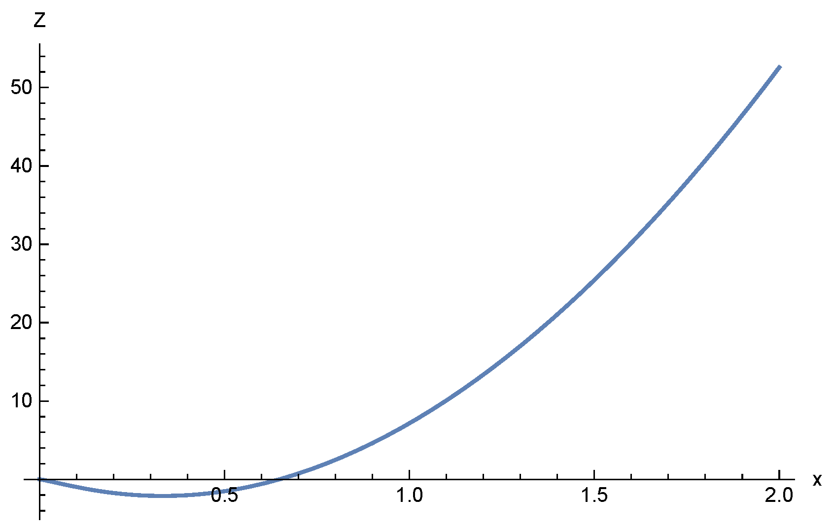
Figure 1. m = M = G = k B = 1 , and x = 1 / T . Plot of Z ( x ) . Here, x = β , G = m = M = 1 . For small x, we see that Z is negative. These x-values are, of course, unphysical. Z grows as T diminishes.
Axioms 10 00121 g001
Figure 2. m = M = G = k B = 1 , and x = 1 / T . Plot of < U ( x ) > . At large temperatures (near the origin), the binding and kinetic energies, as well as the temperature are large, as prescribed by item (1) of the introduction. As T decreases, so does the binding and kinetic energies, as indicated by item (2) of the Introduction.
Axioms 10 00121 g002
Figure 3. Plot of the specific heat C ( x ) . Here, x = β , G = m = M = 1 . It is negative, as prescribed by item (3) of the Introduction. The specific heat tends to vanish as the temperature drops, as expected because of the third law of thermodynamics, that, remarkably enough, is obeyed classically here.
Axioms 10 00121 g003
Figure 4. Plot of Z ( x ) . Here, x = β / R 1 , R 0 = 1 , R 1 = 1000 , G = m = M = 1 .
Axioms 10 00121 g004
Figure 5. Plot of < U ( x ) > . Here, x = β / R 1 , R 0 = 1 , G = m = M = 1 . Note that the size of the container diminishes as x grows, so that the binding energy has to grow with x.
Axioms 10 00121 g005
Figure 6. Plot of C ( x ) versus x. Here, x = β / R 1 , R 0 = 1 , G = m = M = 1 . The binding energy increases as β grows and the mean energy U is negative. Thus, the specific heat = β 2 d U d β is positive. Notably enough, it tends to obey the third law in a classical scenario, as bound by construction.
Axioms 10 00121 g006
Figure 7. Plot of Z ( x ) versus x = β for G = m = R 1 = M = 1 . Results are unphysical for x < 3.35 . At the ensuing very high (big-bang like) temperatures (at which matter does not exist), Z ( x ) is negative, and thus unphysical.
Axioms 10 00121 g007
Figure 8. Plot of < U ( x ) > for x = β G = m = R 1 = M = 1 . Remember that the results are unphysical for x < 3.35 . The kinetic energy diminishes as x grows and so does the energy. However, R 1 is too large to allow for statistical bounding in the region here considered.
Axioms 10 00121 g008
Figure 9. Plot of C ( x ) for x = β . One has G = m = R 1 = M = 1 . Again, the results are unphysical for x < 3.35 . The system tends to comply with the third law. It is unbound, since C > 0 .
Axioms 10 00121 g009
Figure 10. Plot of Z ( x ) for x = β G = m = R 0 = M = 1 . Results turn out to be unphysical for x < 3.35 , as in the previous case.
Axioms 10 00121 g010
Figure 11. Plot of < U ( x ) > for x = β and G = m = R 1 = M = 1 . It closely resembles the companion graph of the precedent case. However, R 0 is too large to allow for statistical bounding in the region here considered.
Axioms 10 00121 g011
Figure 12. Plot of C ( x ) for x = β G = m = R 1 = M = 1 . C > 0 diverges in the unphysical x region. It is positive in the physical one. The third law is complied with.
Axioms 10 00121 g012
Publisher’s Note: MDPI stays neutral with regard to jurisdictional claims in published maps and institutional affiliations.