An Information-Theoretic Framework for Optimal Design: Analysis of Protocols for Estimating Soft Tissue Parameters in Biaxial Experiments

Abstract

A new framework for optimal design based on the information-theoretic measures of mutual information, conditional mutual information and their combination is proposed. The framework is tested on the analysis of protocols—a combination of angles along which strain measurements can be acquired—in a biaxial experiment of soft tissues for the estimation of hyperelastic constitutive model parameters. The proposed framework considers the information gain about the parameters from the experiment as the key criterion to be maximised, which can be directly used for optimal design. Information gain is computed through k-nearest neighbour algorithms applied to the joint samples of the parameters and measurements produced by the forward and observation models. For biaxial experiments, the results show that low angles have a relatively low information content compared to high angles. The results also show that a smaller number of angles with suitably chosen combinations can result in higher information gains when compared to a larger number of angles which are poorly combined. Finally, it is shown that the proposed framework is consistent with classical approaches, particularly D-optimal design.

1. Introduction

Soft tissues exhibit complex biomechanical behaviour, including nonlinearity, anisotropy and heterogeneity [1]. Moreover, the tissues also demonstrate inelastic properties, such as rate-dependence, hysteresis and permanent set. The important link between biomechanics and their physiological function has motivated a large number of ex-vivo studies aimed at characterising their biomechanical properties. Given the complex interplay between the different aspects of their biomechanical properties, the experimental design of ex-vivo soft tissues is extremely challenging and has been a subject of investigation, and a variety of experiments have been proposed [2,3,4,5,6].

Since a variety of soft tissues are thin—e.g., blood vessels, heart valves and skin—biaxial testing is a widely used experimental technique that allows the independent stretching of the tissue in two orthogonal directions and for the corresponding forces to be measured [7,8]. Applying different stretches in two directions allows the characterization of the in-plane anisotropic behavior of a given tissue, while a range of stretches provides us with its nonlinear elastic response. However, even with this relatively simple set of options, the choices of which stretches to apply are unclear. Moreover, it is not obvious upon what these choices will depend.

A variety of hyperelastic models have been developed to describe the anisotropic and nonlinear elastic properties of specific soft tissues [4,9,10,11]. Biaxial experimental data are commonly fit to these models in order to determine the model parameters. As the unknown parameters depend on specific models, the choice of experimental setup—the problem of optimal design—might depend on the choice of model. However, in practice, a predetermined set of experimental protocols is used.

In the present work, an optimal design problem is defined to find the most suitable protocol in view of estimating the parameters of the material model. A comprehensive overview of the optimal design problem can be found in [12,13], and several criteria for optimal design have been proposed in the literature, often based on the minimisation of the variance of the parameters and sensitivities [14,15]. In the present work, we investigate a criterion based on information theoretic quantities, in the spirit of what has been proposed in [16,17] (from a Bayesian point of view) and [18]. Several works have recently proposed information-based criteria to better define experimental protocols. In [19], the authors proposed the maximisation of the mutual information between the parameters and the observations under the assumption that the model error is a Gaussian process. In [20], the authors proposed a framework based on mutual information maximisation to deal with the design of chemistry experiments. The same criterion is proposed in [21]; the authors maximise the mutual information by using a stochastic gradient ascent method. An application to system biology is investigated in [22]. In [23], the maximisation of the information is exploited in order to choose high-fidelity model resolutions in a multi-fidelity modelling framework.

While mutual information has been used for optimal design in previous studies, the novelty of this work is in the proposal of a combination of information-theoretic quantities of both mutual and conditional mutual information. A further novelty is the application of this framework in the optimal design of soft tissue experiments. Estimating information-theoretic quantities is in general a challenging problem, and this is especially the case in high-dimensional settings. In the present work, a model reduction method is coupled with non-parametric sample-based mutual information estimation in order to provide a pertinent estimation of the information-theoretic quantities involved in the optimal design problem and then apply this to the biaxial testing of soft tissues.

The structure of the work is as follows: in Section 2, the model and information-theoretical aspects of the problem are introduced. In particular, in Section 2.1, we detail the mathematical model of the biaxial experiments for soft tissues: after having introduced the notation and the non-linear elasticity model, in Section 2.1.1, we apply it to the biaxial testing experimental setup. In Section 2.1.2, we introduce the experimental protocol definition; the second part of the section is devoted to the description of the information-theoretic framework used to solve the optimal design problem. In Section 2.2.1, we introduce the problem; in Section 2.2.2 and Section 2.2.3, the information-theoretic quantities and their numerical estimation are detailed. We then present the reduce order modeling method used and how to validate the results obtained by the proposed approach. The section ends with an overview of the method. The results and the discussion are presented in Section 3, followed by the conclusion and perspectives on future work.

2. Methods

The methodological aspects are divided into two broad categories: the mathematical model of the biaxial experiments and the information-theoretic optimal design framework.

2.1. Mathematical Model of the Biaxial Experiments

We begin by defining the notation: a material point at its reference position $\mathit{X}\in {\mathbb{R}}^3$ moves to $\mathit{x}\in {\mathbb{R}}^3$ after deformation. The elastic behaviour of soft tissues is described using the hyperelastic strain energy density $\mathsf{\Psi }$, which depends on the deformation gradient tensor $\mathbf{F}={\nabla }_{\mathit{X}}\mathit{x}$. The ratio of the volume after deformation to that before deformation is given by $J=det\left(\mathbf{F}\right)$. Soft tissues are commonly regarded as incompressible due to their high water content; i.e. J is constrained to be unity.

We consider the hyperelastic model proposed by Gasser et al. [24], which defines the strain energy density as

$$\mathsf{\Psi }=\frac{k_1}{2k_2}\left[e^{k_2\left(\kappa I_1+(1-3\kappa )I_4-1\right)}-1\right]+\mu (I_1-3),$$

(1)

where $I_1=tr\left({\mathbf{F}}^{\top }\mathbf{F}\right)$ is the first invariant of the right Cauchy–Green strain tensor $\mathbf{C}={\mathbf{F}}^{\top }\mathbf{F}$ and $I_4=\mathit{M}·\mathbf{C}\mathit{M}$ is the fourth invariant representing the stretch along fiber direction $\mathit{M}$. The resulting Cauchy stress is given by

$$\sigma =2\mathbf{F}·{\displaystyle \frac{\partial \mathsf{\Psi }}{\partial \mathbf{C}}}·{\mathbf{F}}^{\top }-p\mathbf{I},$$

(2)

where p acts as the Lagrange multiplier to enforce incompressibility and $\mathbf{I}$ is the identity matrix.

For this model, the set of unknown parameters can be written as $\left\{k_1,k_2,\kappa ,\mu \right\}$, assuming that the fiber direction $\mathit{M}$ is known a priori (based on another experiment; e.g., light scattering [6]). $\kappa$ represents the dispersion of collagen fibers, which is usually measured from optical experiments. Its value lies between 0 (perfectly anisotropic) and $1/3$ (perfectly isotropic). The value of $\mu$ corresponds to the shear modulus of the neo-Hookean term in (1), which represents the amorphous and non-fibrous extracellular matrix. Its role in the mechanics of soft tissues is limited to small strains and is largely constant across different tissues. In this paper, in order to simplify the problem, we assume that $\kappa =0.1$ and $\mu =1$ kPa are known and fixed. Thus, the aim of an ex-vivo biomechanical experiment is to determine parameters $k_1\in \left[5,100\right]$ kPa and $k_2\in \left[5,80\right]$ robustly and with high confidence [25,26]. A commonly used experiment called biaxial testing is described bellow.

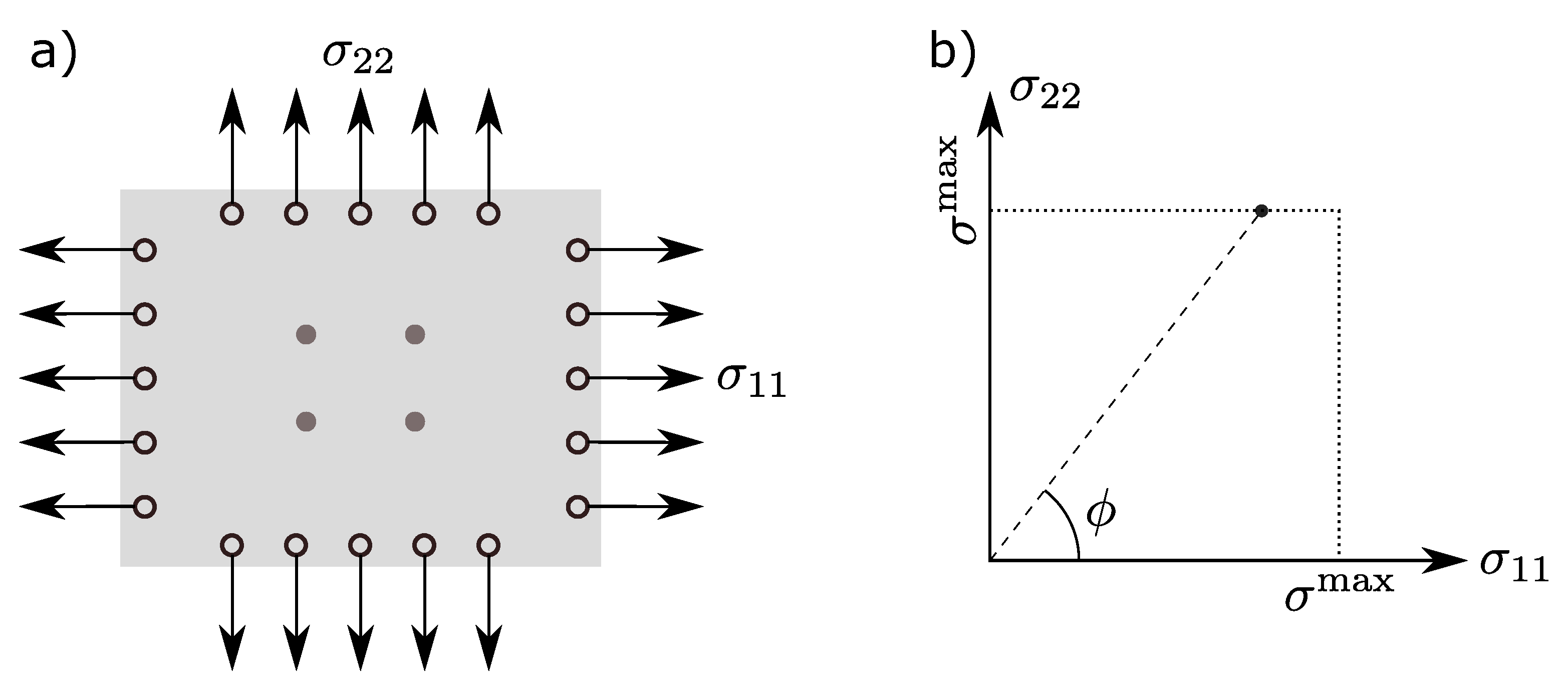
2.1.1. Biaxial Experiments for Soft-Tissues

Many of the soft tissue types are planar with a small thickness. In a biaxial experiment, a square-shaped tissue sample is mounted via clamps or rakes and stretched along two orthogonal directions aligned with the sample edges (Figure 1a). If these directions are used as the two coordinate axes and incompressibility is assumed, the stretching results in a diagonal deformation gradient tensor:

$$\mathbf{F}=diag\left[{\lambda }_1,{\lambda }_2,{\displaystyle \frac{1}{{\lambda }_1{\lambda }_2}}\right],$$

(3)

where ${\lambda }_1$ is the stretch along the first in-plane direction and ${\lambda }_2$ is the stretch along the second in-plane direction. The fiber direction $\mathit{M}$ is generally aligned with the first coordinate axis, which results in only normal stress components. As no force is applied along the thickness of the tissue, ${\sigma }_{33}=0$ is used to determine the Lagrange multiplier p. Thus, we obtain

$$\begin{array}{cc}\hfill {\sigma }_{11}& =2{\displaystyle \frac{\partial \mathsf{\Psi }}{\partial I_1}}\left[{\lambda }_1^2-\frac{1}{{\lambda }_1^2{\lambda }_2^2}\right]+2{\displaystyle \frac{\partial \mathsf{\Psi }}{\partial I_4}}{\lambda }_1^2\hfill \end{array}$$

(4)

$$\begin{array}{cc}\hfill {\sigma }_{22}& =2{\displaystyle \frac{\partial \mathsf{\Psi }}{\partial I_1}}\left[{\lambda }_2^2-\frac{1}{{\lambda }_1^2{\lambda }_2^2}\right].\hfill \end{array}$$

(5)

The applied stresses ${\sigma }_{11}$, ${\sigma }_{22}$ are controlled using load cells. The resulting strains, defined as $e_1:={\lambda }_1-1$ and $e_2:={\lambda }_2-1$, are measured from the marker positions (although $e_1$ and $e_2$ are not the usual strain measures, we use these as our observations). It is important to note that a homogeneous stress and strain state is assumed in the middle of the sample (Figure 1a). Therefore, an implicit assumption is that the material properties and sample thickness are homogeneous. Moreover, these measurement techniques carry an error due to the limitations in measurement tools and/or the deviation from homogeneity, incompressibliity and material direction.

2.1.2. Protocol Definition

In practice, there are two approaches to the biaxial experiment: (1) displacement-controlled, where known stretches are imposed and forces are measured; and (2) force-controlled, where known forces are applied and stretches are measured. Generally, the force-controlled approach is used as it is easier to implement. Therefore, in the force-controlled approach, different values of stresses ${\sigma }_{11}$ and ${\sigma }_{22}$ can be applied.

A single-angle biaxial protocol is defined as a straight line in the ${\sigma }_{11}$-${\sigma }_{22}$ space (Figure 1b). That is, the ratio between the two stresses is kept constant while the applied forces are increased until a maximum value ${\sigma }^{\max }=200$ kPa. Thus, for a chosen angle $\varphi$, we apply

$$\begin{array}{cc}\hfill {\sigma }_{11}& =\left\{\begin{array}{cc}\sigma \hfill & \mathrm{if}\varphi \le {\displaystyle \frac{\pi }{4}}\hfill \\ tan\left(\varphi \right)\sigma \hfill & \mathrm{else}\hfill \end{array}\right.\hfill \end{array}$$

(6)

$$\begin{array}{cc}\hfill {\sigma }_{22}& =\left\{\begin{array}{cc}cot\left(\varphi \right)\sigma \hfill & \mathrm{if}\varphi \le {\displaystyle \frac{\pi }{4}}\hfill \\ \sigma \hfill & \mathrm{else}\hfill \end{array}\right.,\hfill \end{array}$$

(7)

where $\sigma \in [0,{\sigma }^{\max }]$. For $\sigma$, 100 linearly spaced observation points between zero and the maximum stress (${\sigma }^{\max }=200$ kPa) are used. The resulting strains are calculated by iteratively solving Equation (5) for ${\lambda }_{1,2}$ and thereby obtaining $e_{1,2}$. In practice, a combination of angles can be successively tested. We refer to this combination as the experimental protocol that needs to be optimally designed.

For each angle, it is easy to acquire large numbers of points as the sample is continuously stretched. However, to vary between angles, it is essential to restart the experiment at zero applied force, which further requires the “pre-conditioning” of the sample by cyclically applying small stretches. This makes it practically difficult to apply an arbitrarily large number of angles. Therefore, in practice, usually only five angles are tested.

2.2. Information-Theoretic Framework for Optimal Design

The problem of optimal design typically refers to the choice of a design of experiments such that the design is optimal with respect to a pre-determined statistical criterion. We propose that the information-theoretic measures naturally define such statistical criteria. The central idea is that information gain [27,28] from an experiment or protocol—as quantified by the information-theoretic quantities of mutual information and conditional mutual information—can be directly used as a reasonable statistical criterion for optimal design. These quantities are described next after presenting the framework for optimal design.

2.2.1. Optimal Design Problem

Consider the following general model:

$$\mathbf{y}=\mathcal{M}\left(\theta \right),$$

(8)

where $\mathcal{M}$ denotes a forward model that takes $\theta \in {\mathbb{R}}^m$ and outputs $\mathbf{y}\in {\mathbb{R}}^n$. Note that $\theta$ may contain initial and boundary conditions of the model and that $\mathbf{y}$ may subsume the output at many time-points in the case of a dynamic system. Subsequently, consider that the measurement model is as follows:

$$\mathbf{z}={\mathcal{H}}_p(\mathbf{y},\theta )+\epsilon ,$$

(9)

where ${\mathcal{H}}_p$ represents the observation operator, $\mathbf{z}\in {\mathbb{R}}^d$ represents the measurement vector, and $\epsilon$ represents the vector of measurement error/noise. Note that the the observation operator ${\mathcal{H}}_p$ depends on the design of experiments, which specifies which quantities are measured. Given a set of possible ${\mathcal{H}}_p=\{{\mathcal{H}}_1,{\mathcal{H}}_2,\cdots ,{\mathcal{H}}_h\}$, and a statistical criterion $\mathcal{S}\left({\mathcal{H}}_p\right)$ to be maximised, the optimal design is given by

$${\widehat{\mathcal{H}}}_p=\underset{{\mathcal{H}}_p}{arg\; max}\mathcal{S}\left({\mathcal{H}}_p\right).$$

(10)

In the case of the biaxial experiments, the model $\mathcal{M}$ represents the model for the force controlled experiment (Section 2.1.1 and Section 2.1.2) and ${\mathcal{H}}_p$ essentially denotes the experimental protocol (see Section 2.1.2) representing the combination of angles—with each representing a straight line in the ${\sigma }_{11}$–${\sigma }_{22}$ plane—along which the strain measurements of $e_1$ and $e_2$ are acquired. With the possible variation of each angle between 0 and $\pi /2$, the set $\mathsf{\Phi }$ of possible angles $\varphi$ is constructed through a uniform discretisation of the space between 0 and $\pi /2$ into $\alpha$ levels; thus,

$$\mathsf{\Phi }=\{{\varphi }_0,{\varphi }_1,\cdots ,{\varphi }_{\alpha }\}.$$

(11)

The possible set of protocols is then given by any combination of elements in $\mathsf{\Phi }$ with the restriction that the number of elements in a protocol must be limited to $\mathcal{C}$. Thus, if $\overline{\mathsf{\Phi }}\subset \mathsf{\Phi }$ is a subset of angles representing a protocol, our set of protocols is given by

$${\mathcal{H}}_p=\left\{\overline{\mathsf{\Phi }}\subset \mathsf{\Phi }|1\le |\overline{\mathsf{\Phi }}|\le \mathcal{C}\right\},$$

(12)

where $|·|$ represents the number of elements in the set. In other words, we choose at least 1 and up to $\mathcal{C}$ elements from $\mathsf{\Phi }$, with the total elements in ${\mathcal{H}}_p$ being

$$|{\mathcal{H}}_p|=\left(\genfrac{}{}{0pt}{}{\alpha }{1}\right)+\left(\genfrac{}{}{0pt}{}{\alpha }{2}\right)\cdots +\left(\genfrac{}{}{0pt}{}{\alpha }{\mathcal{C}}\right).$$

(13)

2.2.2. Information-Theoretic Quantities for Optimal Design

In the framework of Section 2.2.1, we propose that information-theoretic quantities of mutual information and conditional mutual information are a natural choice for the statistical criterion $\mathcal{S}$. Denoting the random variables associated with $\theta$ and $\mathbf{z}$ as $\mathsf{\Theta }$ and $\mathbf{Z}$, respectively, the mutual information (MI) between the parameters $\mathsf{\Theta }$ and the measurements $\mathbf{Z}$ is defined as [27]

$$\mathcal{I}(\mathsf{\Theta };\mathbf{Z})={\int }_{{\mathcal{X}}_{\mathsf{\Theta }}\times {\mathcal{X}}_{\mathbf{Z}}}{p}_{\mathsf{\Theta },\mathbf{Z}}(\theta ,\mathbf{z})\frac{p_{\mathsf{\Theta },\mathbf{Z}}(\theta ,\mathbf{z})}{p_{\mathsf{\Theta }}\left(\theta \right)p_{\mathbf{Z}}\left(\mathbf{z}\right)}d\theta d\mathbf{z},$$

(14)

where $p_X\left(x\right)$ represents the probability density of a random variable X with a realisation $X=x$ and support ${\mathcal{X}}_X$. The mutual information $\mathcal{I}(\mathsf{\Theta };\mathbf{Z})$ quantifies the amount of information that can be gained on average by one random variable—e.g., $\mathbf{Z}$—knowing about the other—e.g., $\mathsf{\Theta }$. Indeed, with this interpretation, MI is a good candidate for the statistical criterion $\mathcal{S}$ for optimal design. For an individual parameter, ${\mathsf{\Theta }}_i$, or indeed for any combination of parameters $\{{\mathsf{\Theta }}_i,{\mathsf{\Theta }}_j\}$, the corresponding information gains can be similarly computed through $\mathcal{I}({\mathsf{\Theta }}_i;\mathbf{Z})$ and $\mathcal{I}(\{{\mathsf{\Theta }}_i,{\mathsf{\Theta }}_j\};\mathbf{Z})$, respectively. Thus, while $\mathcal{I}({\mathsf{\Theta }}_i;\mathbf{Z})$ quantifies the information gain individually for the parameter ${\mathsf{\Theta }}_i$, the quantity $\mathcal{I}(\{{\mathsf{\Theta }}_i,{\mathsf{\Theta }}_j\};\mathbf{Z})$ quantifies information gain for the pair $\{{\mathsf{\Theta }}_i,{\mathsf{\Theta }}_j\}$ jointly. A measure of correlation between the parameters ${\mathsf{\Theta }}_i$ and ${\mathsf{\Theta }}_j$ is, however, missing and is provided by conditional mutual information (CMI), defined as

$$\underset{\mathrm{I}}{\underbrace{\mathcal{I}({\mathsf{\Theta }}_i;{\mathsf{\Theta }}_j|\mathbf{Z})}}=\underset{\mathrm{II}}{\underbrace{\mathcal{I}({\mathsf{\Theta }}_i;\{{\mathsf{\Theta }}_j,\mathbf{Z}\})}}-\underset{\mathrm{III}}{\underbrace{\mathcal{I}{({\mathsf{\Theta }}_i;\mathbf{Z})}_{\phantom{j}}}}.$$

(15)

The CMI $\mathcal{I}({\mathsf{\Theta }}_i;{\mathsf{\Theta }}_j|\mathbf{Z})$ represents the additional information gained about the parameter ${\mathsf{\Theta }}_i$ when both ${\mathsf{\Theta }}_j$ and Z are known (term II) relative to when only the measurements ${\mathsf{\Theta }}_i$ alone are known (term III). Note that CMI is symmetrical—i.e., $\mathcal{I}({\mathsf{\Theta }}_i;{\mathsf{\Theta }}_j|\mathbf{Z})=\mathcal{I}({\mathsf{\Theta }}_j;{\mathsf{\Theta }}_i|\mathbf{Z})$—and can be interpreted as a measure of dependence between the parameters given the measurements $\mathbf{Z}$. It should also be noted that both MI and CMI are non-negative.

With the above background, many statistical measures can be constructed. For example:

• The mutual information for any single parameter may be maximised, giving $\mathcal{S}=\mathcal{I}({\mathsf{\Theta }}_i;\mathbf{Z})$. This approach only concerns the posterior of the parameter ${\mathsf{\Theta }}_i$ and ignores all other parameters;
• The joint mutual information may be maximised, giving $\mathcal{S}=\mathcal{I}(\mathsf{\Theta };\mathbf{Z})$. In the sense of classical optimal design, this can be interpreted as D-optimal design. This is because D-optimal designs minimise the determinant of the inverse Fisher Information Matrix, and $\mathcal{S}=\mathcal{I}(\mathsf{\Theta };\mathbf{Z})$ measures the information gain in the joint $\mathsf{\Theta }$ space;
• The sum of individual parameter mutual information may be be maximised, giving $\mathcal{S}={\sum }_{i=1}^m\mathcal{I}({\mathsf{\Theta }}_i;\mathbf{Z})$. In the sense of classical optimal design, this can be interpreted as A-optimal design. This is because A-optimal design minimises the trace of the inverse Fisher Information Matrix, and $\mathcal{S}={\sum }_{i=1}^m\mathcal{I}({\mathsf{\Theta }}_i;\mathbf{Z})$ measures the sum of the information gains for all the parameters;
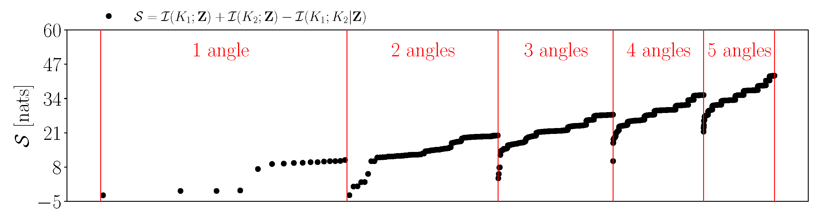
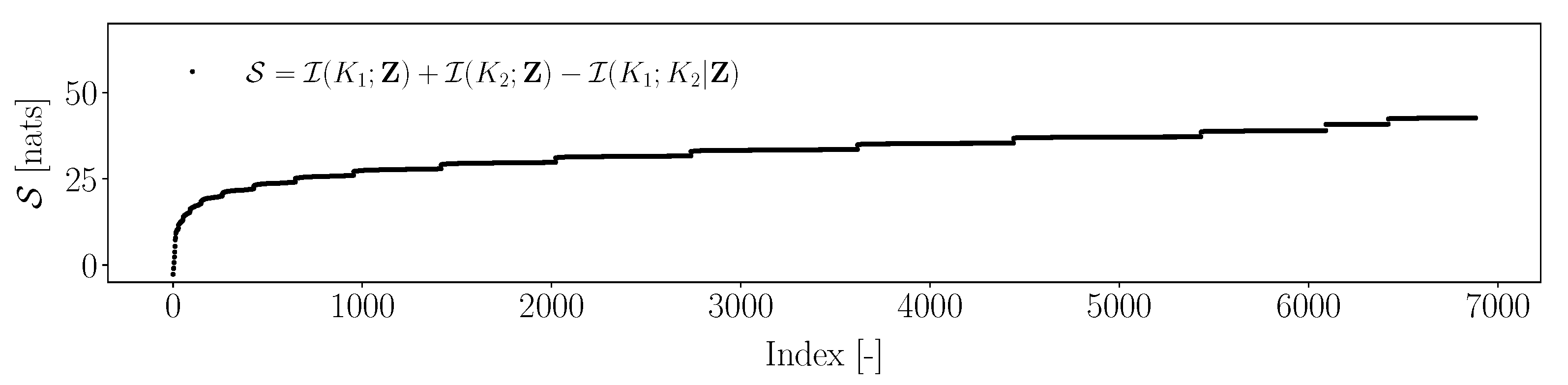
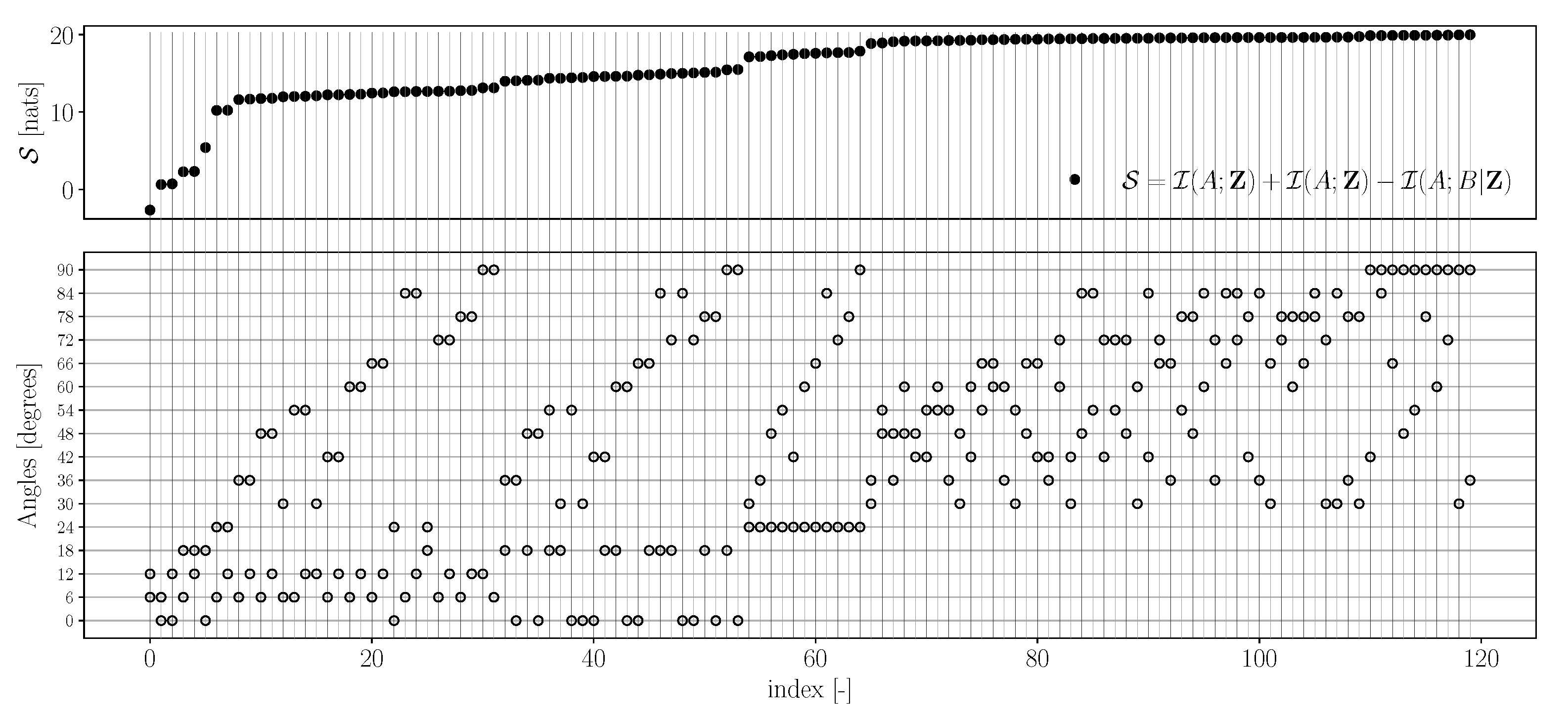
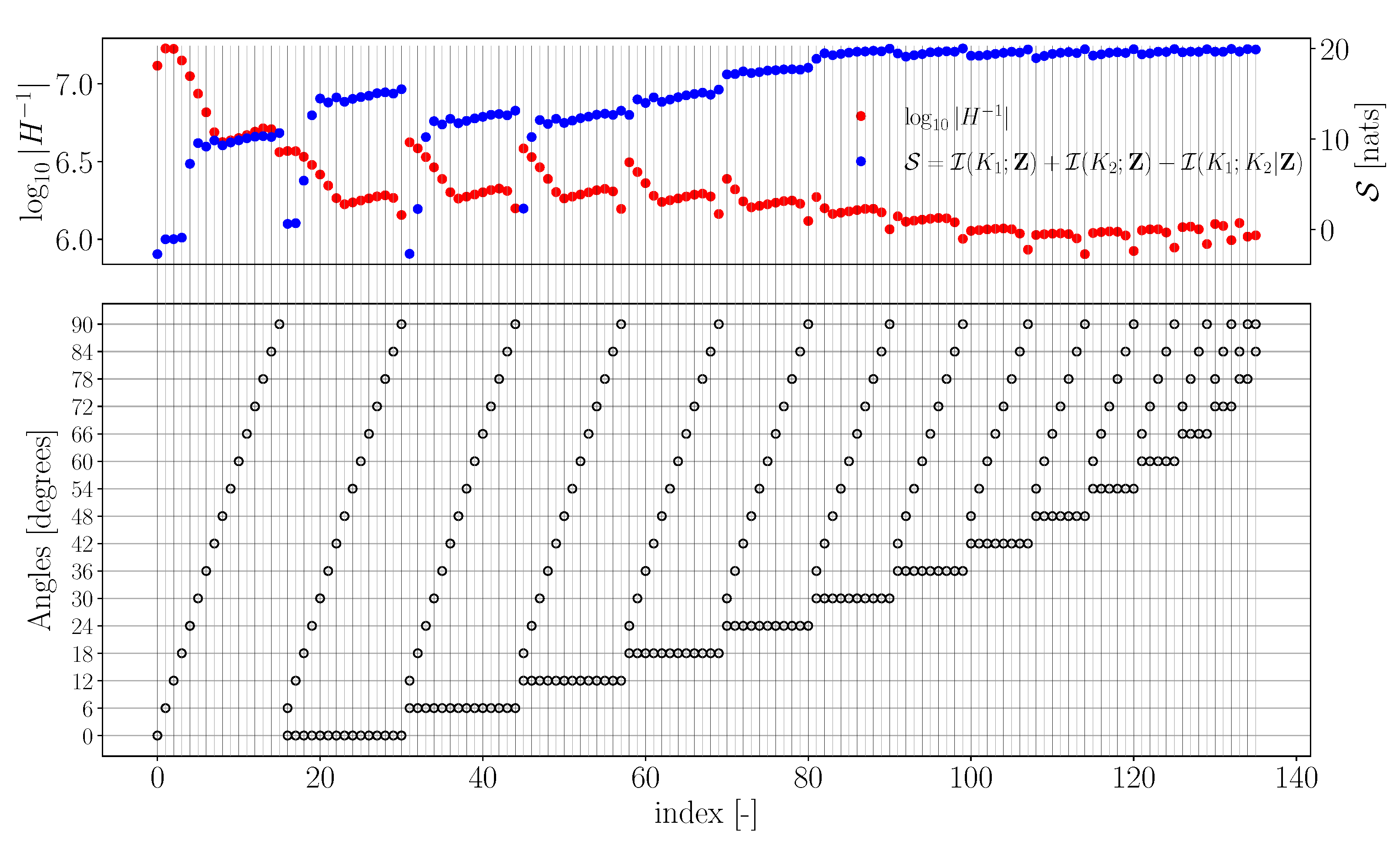
• Alternatively, one may seek to maximise individual parameter information gain while minimising pairwise CMI, thus seeking both small posterior variances and minimising pairwise correlations between the parameters. In this case, the statistical criterion is

  $$\mathcal{S}=\sum _{i=1}^m\mathcal{I}({\mathsf{\Theta }}_i;\mathbf{Z})-\tau \sum _{i=1}^m\sum _{j=i}^m\mathcal{I}({\mathsf{\Theta }}_i;{\mathsf{\Theta }}_j|\mathbf{Z}),$$

  (16)

  where $\tau >0$ is a regularisation parameter. Note that high CMI implies that a large amount of information can be gained only about a combination of the two parameters (for instance, their sum or product), but not for each parameter individually. Thus, we seek to minimise the CMI.

Note that the above list is not exhaustive, and based on the interpretations of MI and CMI, other criteria may be constructed based on the desired sense of optimality.

2.2.3. Estimating Mutual Information

In general, the forward model in Equation (8) is non-linear, and thus even if the observation operator is linear (implying linear combinations of the state are measured), the analytical computation of mutual information is intractable. Thus, the information-theoretic quantities of MI and CMI must be estimated. A common method is to generate samples of $\mathsf{\Theta }$ through the specification of an appropriate prior probability density $p_{\mathsf{\Theta }}\left(\theta \right)$. Denoting these $N_s$ samples as ${\theta }^{\left(i\right)},i=\{1,2,\cdots N_s\}$, each ${\theta }^{\left(i\right)}$ can be propagated through the forward and observation models of Equations (8) and (9) to produce corresponding samples of $\mathbf{Z}$, denoted as ${\mathbf{z}}^{\left(i\right)}$. The samples of ${\theta }^{\left(i\right)}$ and ${\mathbf{z}}^{\left(i\right)}$ can subsequently be used on non-parametric estimators of MI and CMI. Such non-parametric estimators can broadly be classified into two categories: kernel density estimators (KDE) [29] and k-nearest neighbour (kNN) estimators [30,31]. For an overview of such methods, we refer to [32]. While the estimator proposed by Kraskov et. al. [30] is widely used and performs very well across a range of scenarios, one of its drawbacks is that it suffers from higher errors when extreme correlations are present between the variables and/or when the the data are effectively in a lower-dimensional manifold. Since we are working with models that specify explicit relationships between the variables through the forward and observation model, this is likely to be true for the data set of $({\theta }^{\left(i\right)},{\mathbf{z}}^{\left(i\right)})$. Thus, in this study, we employ the local non-uniformity correction (LNC) proposed in [33], which includes a correction term to the original estimator by Kraskov et al. [30]. This term accounts for strong dependencies between the variables through local principle component analysis [33]. The method of [33] is used for the estimation of all MIs, and CMIs are estimated from the difference of two MIs; see Equation (15).

2.2.4. Dimensionality Reduction for the Biaxial Experiment

One of the main difficulties in estimating information-theoretic quantities is related to the data dimension. Non-parametric estimation is particularly challenging whenever the data are close to manifolds embedded in high-dimensional spaces. This is indeed the case when a physical model relates parameters and observable quantities. One of the possible ways to overcome this difficulty, or at least to mitigate it, is (dimension or) model reduction, which aims at discovering the underlying low-dimensional structure of a set of data (a comprehensive review of the topic can be found in [34,35,36,37]). A large spectrum of methods has been proposed in the literature. In the present contribution, we adopt a local reduced-basis method (similar in spirit to the methods proposed in [38,39]). Let the strains computed by the model be $e_{1,2}(\sigma ;\varphi ;k_1,k_2)$, where $k_1$ and $k_2$ are the model parameters $(k_1,k_2)\in {\mathsf{\Omega }}_k\subset {\mathbb{R}}^2$, and $\sigma \in {\mathsf{\Omega }}_{\sigma }\subset \mathbb{R}$ is the variable defined in Section 2.1.2. Let $n\in {\mathbb{N}}^{*}$; thus, we introduce the following approximation:

$$e_{1,2}\approx \sum _{i=1}^n{\eta }_i{r}_i(\sigma ,\varphi )s_i(k_1,k_2,\varphi ),$$

(17)

which is well defined by virtue of the Eckart–Young theorem. First, let us observe that a given protocol consists of a set of known angles $\overline{\mathsf{\Phi }}$. An efficient way to construct the local reduced basis is therefore to introduce a Proper Orthogonal Decomposition (POD) for each of the angles ${\varphi }_j\in \overline{\mathsf{\Phi }}$. This corresponds to the search for an approximation of the form

$$e_{1,2}^{\left(j\right)}(\sigma ;{\varphi }_j;k_1,k_2)\approx \sum _{i=1}^n{\eta }_i^{\left(j\right)}{r}_i^{\left(j\right)}\left(\sigma \right)s_i^{\left(j\right)}(k_1,k_2),$$

(18)

where ${\langle r_i^{\left(j\right)},r_k^{\left(j\right)}\rangle }_{{\mathsf{\Omega }}_{\sigma }}={\delta }_{ik}$ and ${\langle s_i^{\left(j\right)},s_k^{\left(j\right)}\rangle }_{{\mathsf{\Omega }}_k}={\delta }_{ik}$ (${\langle ·,·\rangle }_{{\mathsf{\Omega }}_{\sigma },with{\mathsf{\Omega }}_k}$ being the standard $L^2$ scalar product). The error in the approximation is related to the number n of modes retained:

$$\parallel e_{1,2}^{\left(j\right)}-\sum _{i=1}^n{\eta }_i^{\left(j\right)}{r}_i^{\left(j\right)}\left(\sigma \right)s_i^{\left(j\right)}(k_1,k_2){\parallel }_{L^2({\mathsf{\Omega }}_{\sigma }\times {\mathsf{\Omega }}_k)}^2=\sum _{i=n+1}^{\infty }{{\eta }_i^{\left(j\right)}}^2$$

(19)

In the present work, a number $n=4$ of modes proved to be sufficient in order to obtain errors smaller than ${10}^{-3}$ in $L^2$ norm in the solution reconstruction. This means that the set of elements $e_{1,2}(\sigma ;{\varphi }_j;k_1,k_2)$ was close to the linear subspace spanned by the first $n=4$ modes $r_i^{\left(j\right)}$. Henceforth, instead of considering the discretised $e_{1,2}$ we consider their coordinates in the subspace given by

$$z_{1,2}^{\left(j\right)}{|}_i={\langle e_{1,2},r_i^{\left(j\right)}\rangle }_{{\mathsf{\Omega }}_{\sigma }}={\eta }_i^{\left(j\right)}{s}_i^{\left(j\right)}(k_1,k_2).$$

(20)

2.2.5. Validation of Results against Existing Methods

Several methods and criteria to define and reach an optimal design of experiments have been proposed [12]. Among them, D–optimality criterion attempts at maximising the determinant of the information matrix. In the present case, this is equivalent to minimize the determinant of the inverse of the average Hessian of the loss function we would introduce in a classical parameter estimation method. In a noisy setting, and, in particular, when the noise is Gaussian, this cost function is equivalent to minus the logarithm of the likelihood function. Let the misfit function be $f\left(\theta \right)$ and ${\mathbb{E}}_{\mathsf{\Theta }}$ denote the expectation operator. The average of the Hessian reads:

$$H={\mathbb{E}}_{\mathsf{\Theta }}\left[{\partial }_{\theta }^{2}f{|}_{{\theta }_{*}}\right],$$

(21)

where ${\theta }_{*}$ is the value of the parameter minimising the loss function.

2.2.6. Overview of Approach for the Biaxial Experiments

In the context of the biaxial experiments, the parameters are $k_1$ and $k_2$, represented as random variables $K_1$ and $K_2$, respectively. The variability in these parameters is considered to be uniform (thus imposing a uniform prior distribution) in the following intervals: $k_1\in [5,100]$ kPa and $k_2\in [5,80]$. For a single value of angle $\varphi$, the measurements are the strain values $e_1$ and $e_2$ and are measured at 100 points along the line defined by the angle $\varphi$. Here, we consider $\alpha =16$ discrete values of possible measurement angles $\varphi$ uniformly distributed between, and including, 0${}^{\circ }$ and 90${}^{\circ }$. For each angle $\varphi$, separate reduced bases of four modes for $e_1$ and $e_2$ are constructed through POD over 400 values of $(K_1,K_2)$ sampled uniformly in the aforementioned parametric space. Thus, for any angle $\varphi$, the dimensionality reduction approach projects $e_1$ and $e_2$ measured at 100 points along the line defined by $\varphi$ to a basis of 4 + 4 modes. For a given protocol consisting of multiple angles, the measurement vector $\mathbf{z}$ (with a corresponding random variable $\mathbf{Z}$) is the collection of all the reduced basis representations of $e_1$ and $e_2$ along the angles in the protocol. Lastly, the maximum number of angles in a protocol is restricted to $\mathcal{C}=5$, giving a total of 6884 unique combinations of the $\alpha =16$ angles.

For the estimation of MI and CMI, a total of $N=\mathrm{10,000}$ values of $(K_1,K_2)$ are uniformly distributed in the parametric space. For each sample $(k_1^{\left(i\right)},k_2^{\left(i\right)})$, the numerical model of the biaxial experiment is run to produce $e_1^{\left(i\right)}$ and $e_2^{\left(i\right)}$, which are then projected on to the reduced basis, giving ${\mathbf{z}}^{\left(i\right)}$. The N triplets of $(k_1^{\left(i\right)},k_2^{\left(i\right)},{\mathbf{z}}^{\left(i\right)})$ are subsequently used for the estimation of MI and CMI through the LNC estimator (see Section 2.2.3). In Equation (16), we use $\tau =1$.

3. Results and Discussion

For all the 6884 combinations of angles, three statistical criteria are evaluated: (i) $\mathcal{I}(K_1;\mathbf{Z})$, (ii) $\mathcal{I}(K_2;\mathbf{Z})$ and (iii) $\mathcal{I}(K_1;\mathbf{Z})+\mathcal{I}(K_2;\mathbf{Z})-\mathcal{I}(K_1;K_2|\mathbf{Z})$. While the first two criteria aim to maximise the information gain about $K_1$ and $K_2$ individually, the third criterion aims to maximise the information gain about $K_1$ and $K_2$ simultaneously while minimising the information dependence between them. Figure 2, Figure 3 and Figure 4 show the variation in these three criteria when grouped by the number of angles in a protocol. In these figures, the values of information criterion when using two approaches to uniformly discretise the angular space within protocols are also presented. Observations from these plots are as follows:

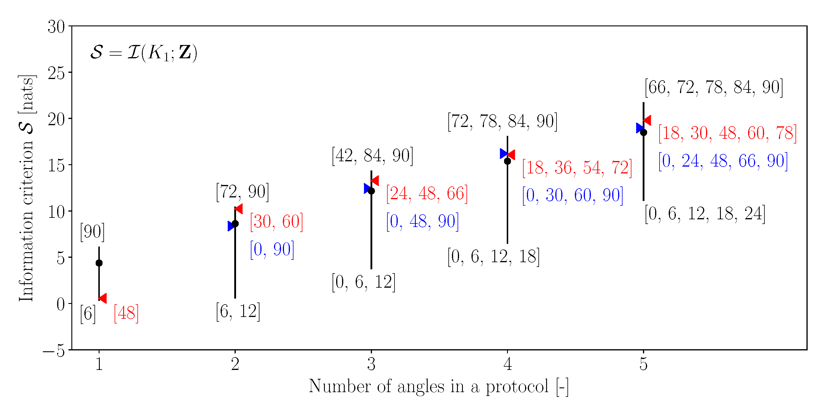
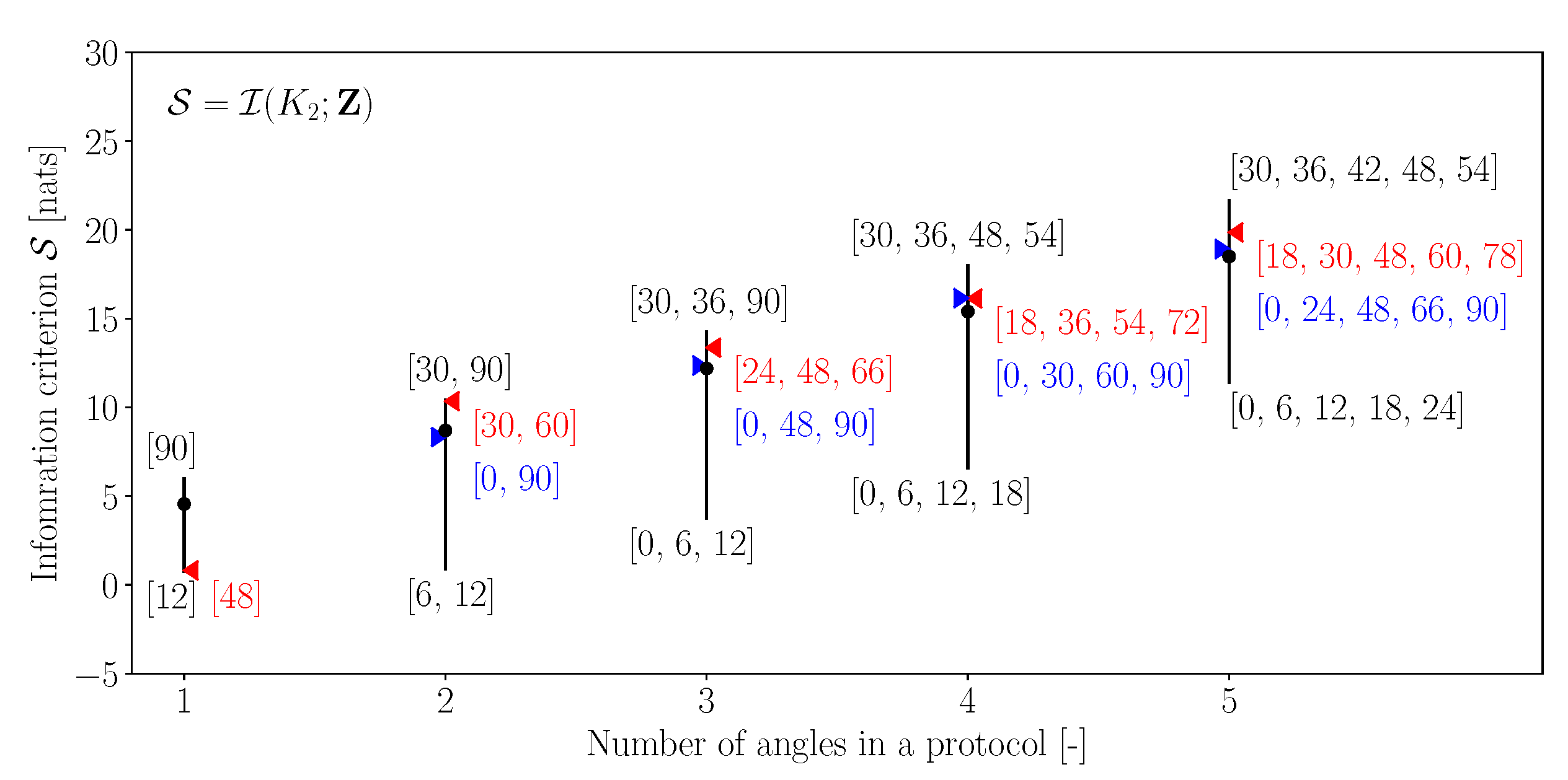
• Generally, all the three information criteria increase with the increasing number of angles in the protocol. Intuitively, this is expected, as a higher number of angles implies more measurement data and hence a higher potential for the improved estimation of the parameters. This observation is true for the maximum information gain, minimum information gain and the mean information gain;
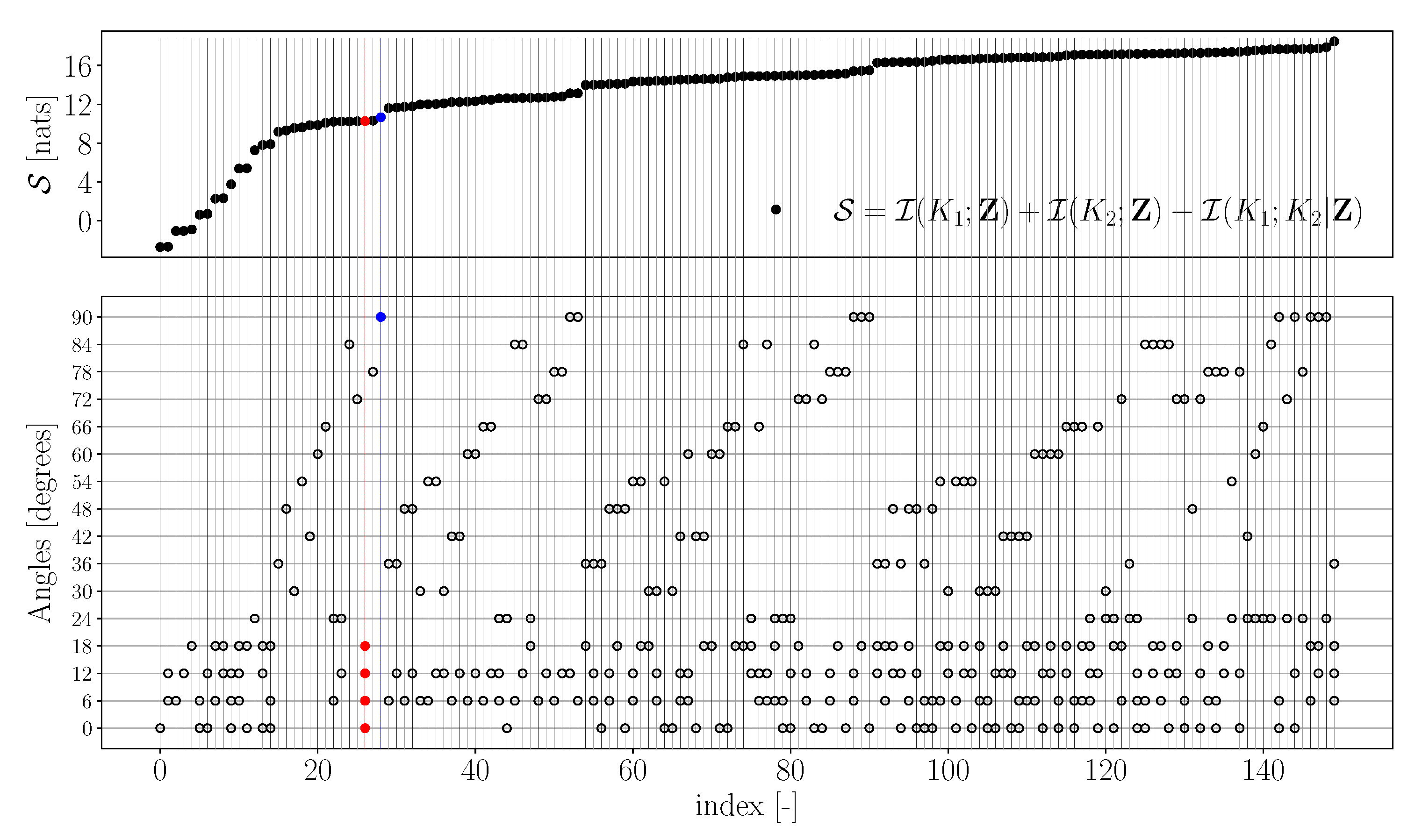
• Across all the three criteria, it is observed that the uniform discretisation is not necessarily reflective of the best protocol for estimating the parameters. In fact, in most cases, the performance of uniform discretisation is close to the mean information gain observed across all the angle combinations;
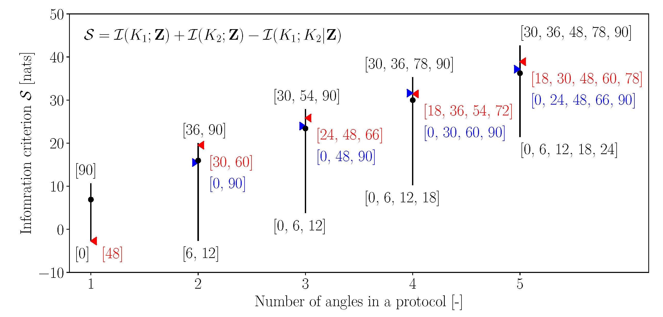
• From Figure 2 and Figure 3, it is observed that the angular combinations that maximise information gain for $K_1$ are not identical—and vary significantly when more than two angles are simultaneously used—to those that maximise information gain for $K_2$. This further motivates the use of a criterion that balances information gains in both the parameters while minimising their interdependence;
• Figure 4 shows that the best combinations that maximise a balanced criterion, such as $\mathcal{I}(K_1;\mathbf{Z})+\mathcal{I}(K_2;\mathbf{Z})-\mathcal{I}(K_1;K_2|\mathbf{Z})$, are a trade-off between the combinations of angles that maximise $\mathcal{I}(K_1;\mathbf{Z})$ and $\mathcal{I}(K_2;\mathbf{Z})$ individually. For example, when five angles are considered, the angles that maximise $\mathcal{I}(K_1;\mathbf{Z})$ are ${\varphi }_a=[66,72,78,84,90]$ and those that maximise $\mathcal{I}(K_2;\mathbf{Z})$ are ${\varphi }_b=[30,36,42,48,54]$, while the combination that maximises $\mathcal{I}(K_1;\mathbf{Z})+\mathcal{I}(K_2;\mathbf{Z})-\mathcal{I}(K_1;K_2|\mathbf{Z})$ is $[30,36,48,78,90]$, which has two angles from ${\varphi }_a$ and three angles from ${\varphi }_b$. It should be noted that such a trade-off between maximising individual parameter gains is still significantly different to a uniform discretisation;
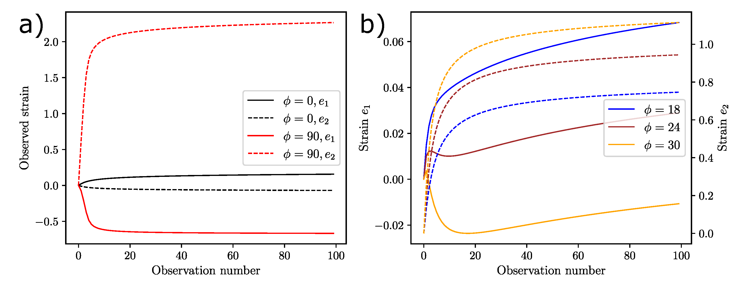
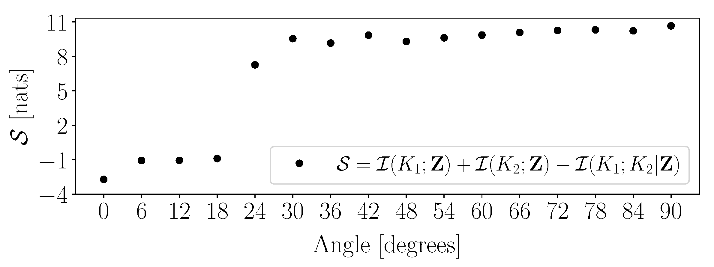
• Finally, it is observed that the worst combinations are all low angles: $[0,6,12,18,24]$. This can be related to the fact that, at low angles, the applied stress is largely aligned along the stiff fibers of the tissue, thus resulting in lower strain values. Thus, the lower angles provide a small range of the observations, while the larger angles provide a larger range (Figure 5a), thereby containing more information about the parameters.

From this point onward, we present results only for the balanced information criterion $\mathcal{S}=\mathcal{I}(K_1;\mathbf{Z})+\mathcal{I}(K_2;\mathbf{Z})-\mathcal{I}(K_1;K_2|\mathbf{Z})$. Figure 6 shows the variation in $\mathcal{S}$ across all the combinations (x-axis and in log-scale to capture the spread) grouped by the number of angles in a protocol and sorted according to the increasing order of $\mathcal{S}$ within each such group. Within each group, observing the minimum and maximum values of $\mathcal{S}$ shows that a better choice of angles can lead to more than a 100% increase in the information gain compared to a poor choice. Furthermore, this shows that good combinations of a lower number of angles can lead to higher information gain compared to a higher number of angles with poor combinations. For example, the maximum $\mathcal{S}$ when only one angle is used is higher than many combinations with two to four angles. This emphasises the utility of optimal design and the proposed framework.

Figure 7 shows $\mathcal{S}$ for all the 6884 combinations in increasing order of magnitude, and Figure 8 shows a zoomed plot for the first 150 combinations along with the corresponding combinations of angles. Observing the index values of 26 (red) and 28 (blue) in Figure 8 shows that even though four combinations are used in the index 26 protocol, it produces a lower $\mathcal{S}$ compared to when only a single angle is used in the index 28 protocol. Furthermore, since Figure 8 shows the first 150 out of 6884 combinations of Figure 7 (which is sorted in creasing order of $\mathcal{S}$), all combinations here are relatively low $\mathcal{S}$-producing protocols. Observing the high density of angles in the region $\varphi <{24}^{\circ }$ is indicative that lower values of angles—in particular, those less than 24${}^{\circ }$—are relatively less informative when compared to higher values of angles. This behaviour is also apparent in Figure 9, which shows $\mathcal{S}$ values for protocols that use only one angle, and where a sharp jump can be observed when transitioning from 18${}^{\circ }$ to 24${}^{\circ }$. This peculiar behaviour may be explained by the physics of the biaxial experiment. Looking at the resulting strains $e_1$ and $e_2$ of this transition (Figure 5b), we observe that the $e_1$ changes from positive to negative values. This behavior captures the important coupling between the two normal stresses and strains and is also related to the fiber dispersion in our constitutive model (Equation (1), [24]). It is remarkable and encouraging that the information-theoretic framework captures the physics of the problem without explicitly considering it in the framework. While for simpler low-dimensional models, the association between physics and optimal design may be relatively easy to see, inferring such behaviour is, in general, not trivial for more complex and higher-dimensional models.

Similarly to Figure 9, the results of the information-theoretic optimal design are further analysed for a higher number of angles. When two angles are considered, the $\mathcal{S}$ values in increasing order of magnitude and the corresponding angle combinations are shown in Figure 10. This figure re-iterates observations made previously: (i) the choice of combinations significantly affects the information gain, where the best combination gives approximately 20 nats more information compared to the worst combination; and (ii) generally speaking, higher angles are more informative compared to lower angles—in particular, angles below 24${}^{\circ }$. While a similar analysis for more than two angle combinations can be easily performed, the efficient visual representation of such results is cumbersome and avoided in this manuscript.

To further illustrate the validity of the information-theoretic approach, a comparison with a classical method (see Section 2.2.5) is presented. For one and two angles in a protocol, Figure 11 shows a comparison between $\mathcal{S}$ and the log of the determinant of the inverse Fisher Information Matrix, $log|H^{-1}|$. It is encouraging that a high correspondence between the two metrics is observed. In particular, increases in $\mathcal{S}$, implying higher information gains, are accompanied by corresponding decreases in $log|H^{-1}|$, implying a smaller volume of the parameter posteriors. A Pearson correlation coefficient of $r=-0.76$ is observed between $\mathcal{S}$ and $log|H^{-1}|$, implying a high similarity between the two metrics and validating the information-theoretic approach in part. We note that, when the number of the parameters become large, evaluating the Hessian would imply a non-negligible computational cost. On the contrary, the method used to evaluate the mutual information, as a primarily Monte Carlo-based estimation, is less severely dependent on the number of parameters. Furthermore, the computation of derivatives (either numerically or through adjoint based methods) may be cumbersome for certain types of models. Finally, we note that the effect of noise on information gain, and hence optimal design, can be easily assessed in the proposed framework by adding noise to the samples of $\mathbf{Z}$ (see Equation (9)).

4. Conclusions

A framework for optimal design based on information-theoretic quantities of mutual information and conditional mutual information is proposed. The framework treats information gain as the central criterion for inverse problems and proposes several information-theoretic frameworks for a desired sense of optimality. The capabilities of this framework are tested on the optimal design problem for biaxial experiments, where the effect of the angle combinations along which the strains are measured is assessed in terms of parameter estimation through information gain. Without including any physics-based reasoning, and purely through the information-theoretic measures, it is found that low angles $\le {24}^{\circ }$ are not very informative regarding the parameters relative to high angles. These observations are then found to be consistent based on physics-based reasoning, thereby showing the efficacy of the proposed framework. Furthermore, it is demonstrated that measurements for a low total number of angles which are carefully chosen can be more informative compared to the case when measurements along a high number of poorly chosen angles are acquired, thus highlighting both the importance of optimal design for biaxial experiments and the utility of the proposed framework in determining good angle combinations. The application of the proposed framework to classical optimal design is performed, and it is shown that the results produced by the new framework are consistent with classical frameworks.

5. Limitations and Future Work

While the proposed framework is shown to perform well on a two-parameter problem, its performance in higher parameter problems is not assessed. This assessment represents the primary limitation of this work and an area of future assessment. In particular, the problems envisaged are largely related to the performance of the MI and CMI estimators in higher dimensions of both parameters and the measurements. While a dimensionality reduction approach was adopted in this study to minimise the adverse effects of the latter, this may not be possible in many forward and inverse problems. Thus, a large area of future work is related to the development of efficient and robust MI and CMI estimators. Note that several approaches are being proposed by researchers to solve this problem; see for example [40,41,42,43,44,45,46]. Lastly, a thorough comparison against classical optimal design methods (C, E, T and V-optimal designs, etc.) needs to be performed, along with the construction and analysis of corresponding information-theoretic metrics.

References

1. Holzapfel, G.A. Nonlinear Solid Mechanics; Wiley: Chichester, UK, 2000; Volume 24. [Google Scholar]
2. Zhang, W.; Feng, Y.; Lee, C.H.; Billiar, K.L.; Sacks, M.S. A generalized method for the analysis of planar biaxial mechanical data using tethered testing configurations. J. Biomech. Eng. 2015, 137, 064501. [Google Scholar] [CrossRef] [PubMed] [Green Version]
3. Labrosse, M.R.; Jafar, R.; Ngu, J.; Boodhwani, M. Planar biaxial testing of heart valve cusp replacement biomaterials: Experiments, theory and material constants. Acta Biomater. 2016, 45, 303–320. [Google Scholar] [CrossRef]
4. Humphrey, J.; Yin, F. On constitutive relations and finite deformations of passive cardiac tissue: I. A pseudostrain-energy function. J. Biomech. Eng. 1987, 109, 298–304. [Google Scholar] [CrossRef]
5. Laurence, D.; Ross, C.; Jett, S.; Johns, C.; Echols, A.; Baumwart, R.; Towner, R.; Liao, J.; Bajona, P.; Wu, Y.; et al. An investigation of regional variations in the biaxial mechanical properties and stress relaxation behaviors of porcine atrioventricular heart valve leaflets. J. Biomech. 2019, 83, 16–27. [Google Scholar] [CrossRef] [PubMed]
6. Jett, S.V.; Hudson, L.T.; Baumwart, R.; Bohnstedt, B.N.; Mir, A.; Burkhart, H.M.; Holzapfel, G.A.; Wu, Y.; Lee, C.H. Integration of polarized spatial frequency domain imaging (pSFDI) with a biaxial mechanical testing system for quantification of load-dependent collagen architecture in soft collagenous tissues. Acta Biomater. 2020, 102, 149–168. [Google Scholar] [CrossRef] [PubMed]
7. Billiar, K.L.; Sacks, M.S. Biaxial mechanical properties of the native and glutaraldehyde-treated aortic valve cusp: Part II–a structural constitutive model. J. Biomech. Eng. 2000, 122, 327–335. [Google Scholar] [CrossRef] [PubMed]
8. Ross, C.; Laurence, D.; Wu, Y.; Lee, C.H. Biaxial Mechanical Characterizations of Atrioventricular Heart Valves. J. Vis. Exp. JoVE 2019. [Google Scholar] [CrossRef] [PubMed]
9. Maurel, W.; Thalmann, D.; Wu, Y.; Thalmann, N.M. Constitutive Modeling. In Biomechanical Models for Soft Tissue Simulation; Springer: Berlin/Heidelberg, Germany, 1998; pp. 79–120. [Google Scholar]
10. Holzapfel, G.A.; Gasser, T.C.; Ogden, R.W. A new constitutive framework for arterial wall mechanics and a comparative study of material models. J. Elast. Phys. Sci. Solids 2000, 61, 1–48. [Google Scholar]
11. May-Newman, K.; Yin, F.C.P. A constitutive law for mitral valve tissue. J. Biomech. Eng. 1998, 120, 38–47. [Google Scholar] [CrossRef]
12. Pukelsheim, F. Optimal Design of Experiments; Society for Industrial and Applied Mathematics (SIAM): Philadelphia, PA, USA, 2006. [Google Scholar]
13. Banks, H.T.; Holm, K.; Kappel, F. Comparison of optimal design methods in inverse problems. Inverse Probl. 2011, 27, 075002. [Google Scholar] [CrossRef] [PubMed]
14. Banks, H.T.; Dediu, S.; Ernstberger, S.L.; Kappel, F. Generalized sensitivities and optimal experimental design. J. Inv. Ill-Posed Problems. 2010, 18, 25–83. [Google Scholar] [CrossRef] [Green Version]
15. Banks, H.T.; Rubio, D.; Saintier, N.; Troparevsky, M.I. Optimal design techniques for distributed parameter systems. In Proceedings of the 2013 Conference on Control and Its Applications, San Diego, CA, USA, 8–10 July 2013; pp. 83–90. [Google Scholar]
16. Lindley, D.V. On a measure of the information provided by an experiment. Ann. Math. Stat. 1956, 27, 986–1005. [Google Scholar] [CrossRef]
17. Sebastiani, P.; Wynn, H.P. Maximum entropy sampling and optimal Bayesian experimental design. J. R. Stat. Soc. Ser. (Stat. Methodol.) 2000, 62, 145–157. [Google Scholar] [CrossRef]
18. Capellari, G.; Chatzi, E.; Mariani, S. Parameter identifiability through information theory. In Proceedings of the 2nd ECCOMAS Thematic Conference on Uncertainty Quantification in Computational Sciences and Engineering (UNCECOMP), Rhodes Island, Greece, 15–17 June 2017; pp. 15–17. [Google Scholar]
19. Bryant, C.; Terejanu, G. An information-theoretic approach to optimally calibrate approximate models. In Proceedings of the 50th AIAA Aerospace Sciences Meeting including the New Horizons Forum and Aerospace Exposition, Nashville, TN, USA, 9–12 January 2012; p. 153. [Google Scholar]
20. Terejanu, G.; Upadhyay, R.R.; Miki, K. Bayesian experimental design for the active nitridation of graphite by atomic nitrogen. Exp. Therm. Fluid Sci. 2012, 36, 178–193. [Google Scholar] [CrossRef] [Green Version]
21. Huan, X.; Marzouk, Y.M. Simulation-based optimal Bayesian experimental design for nonlinear systems. J. Comput. Phys. 2013, 232, 288–317. [Google Scholar] [CrossRef] [Green Version]
22. Liepe, J.; Filippi, S.; Komorowski, M.; Stumpf, M.P. Maximizing the information content of experiments in systems biology. PLoS Comput. Biol. 2013, 9, e1002888. [Google Scholar] [CrossRef] [PubMed] [Green Version]
23. Lewis, A.; Smith, R.; Williams, B.; Figueroa, V. An information theoretic approach to use high-fidelity codes to calibrate low-fidelity codes. J. Comput. Phys. 2016, 324, 24–43. [Google Scholar] [CrossRef] [Green Version]
24. Gasser, T.C.; Ogden, R.W.; Holzapfel, G.A. Hyperelastic modelling of arterial layers with distributed collagen fibre orientations. J. R. Soc. Interface 2006, 3, 15–35. [Google Scholar] [CrossRef] [PubMed]
25. Aggarwal, A. An improved parameter estimation and comparison for soft tissue constitutive models containing an exponential function. Biomech. Model. Mechanobiol. 2017, 16, 1309–1327. [Google Scholar] [CrossRef] [PubMed] [Green Version]
26. Aggarwal, A. Effect of Residual and Transformation Choice on Computational Aspects of Biomechanical Parameter Estimation of Soft Tissues. Bioengineering 2019, 6, 100. [Google Scholar] [CrossRef] [PubMed] [Green Version]
27. Pant, S.; Lombardi, D. An information-theoretic approach to assess practical identifiability of parametric dynamical systems. Math. Biosci. 2015, 268, 66–79. [Google Scholar] [CrossRef] [Green Version]
28. Pant, S. Information sensitivity functions to assess parameter information gain and identifiability of dynamical systems. J. R. Soc. Interface 2018, 15, 20170871. [Google Scholar] [CrossRef]
29. Moon, Y.I.; Rajagopalan, B.; Lall, U. Estimation of mutual information using kernel density estimators. Physical Rev. E 1995, 52, 2318. [Google Scholar] [CrossRef] [PubMed]
30. Kraskov, A.; Stögbauer, H.; Grassberger, P. Estimating mutual information. Phys. Rev. E 2004, 69, 066138. [Google Scholar] [CrossRef] [PubMed] [Green Version]
31. Lombardi, D.; Pant, S. Nonparametric k-nearest-neighbor entropy estimator. Phys. Rev. E 2016, 93, 013310. [Google Scholar] [CrossRef] [PubMed] [Green Version]
32. Beirlant, J.; Dudewicz, E.J.; Györfi, L.; Van der Meulen, E.C. Nonparametric entropy estimation: An overview. Int. J. Math. Stat. Sci. 1997, 6, 17–39. [Google Scholar]
33. Gao, S.; Ver Steeg, G.; Galstyan, A. Efficient estimation of mutual information for strongly dependent variables. In Proceedings of the Eighteenth International Conference on Artificial Intelligence and Statistics, San Diego, CA, USA, 9–12 May 2015; pp. 277–286. [Google Scholar]
34. Benner, P.; Gugercin, S.; Willcox, K. A survey of projection-based model reduction methods for parametric dynamical systems. SIAM Rev. 2015, 57, 483–531. [Google Scholar] [CrossRef]
35. Benner, P.; Ohlberger, M.; Cohen, A.; Willcox, K. Model Reduction and Approximation: Theory and Algorithms; Society for Industrial and Applied Mathematics (SIAM): Philadelphia, PA, USA, 2017. [Google Scholar]
36. Quarteroni, A.; Rozza, G. Reduced Order Methods for Modeling and Computational Reduction; Springer: Berlin/Heidelberg, Germany, 2014; Volume 9. [Google Scholar]
37. Ma, Y.; Fu, Y. Manifold Learning Theory and Applications; CRC Press: Boca Raton, FL, USA, 2011. [Google Scholar]
38. Amsallem, D.; Haasdonk, B. PEBL-ROM: Projection-error based local reduced-order models. Adv. Model. Simul. Eng. Sci. 2016, 3, 1–25. [Google Scholar] [CrossRef] [Green Version]
39. Maday, Y.; Stamm, B. Locally adaptive greedy approximations for anisotropic parameter reduced basis spaces. SIAM J. Sci. Comput. 2013, 35, A2417–A2441. [Google Scholar] [CrossRef] [Green Version]
40. Belghazi, M.I.; Baratin, A.; Rajeshwar, S.; Ozair, S.; Bengio, Y.; Courville, A.; Hjelm, D. Mutual information neural estimation. In Proceedings of the Machine Learning Research, Stockholmsmässan, Stockholm Sweden, 10–15 July 2018; pp. 531–540. [Google Scholar]
41. Singh, S.; Póczos, B. Generalized exponential concentration inequality for Rényi divergence estimation. In Proceedings of the 31st International Conference on Machine Learning, Bejing, China, 22–24 June 2014; pp. 333–341. [Google Scholar]
42. Kleinegesse, S.; Drovandi, C.; Gutmann, M.U. Sequential Bayesian experimental design for implicit models via mutual information. Bayesian Anal. 2021, 1, 1–30. [Google Scholar] [CrossRef]
43. Fukumizu, K. Nonparametric Bayesian inference with kernel mean embedding. In Modern Methodology and Applications in Spatial-Temporal Modeling; Springer: Berlin/Heidelberg, Germany, 2015; pp. 1–24. [Google Scholar]
44. Moon, K.R.; Hero, A.O. Ensemble estimation of multivariate f-divergence. In Proceedings of the 2014 IEEE International Symposium on Information Theory, Honolulu, HI, USA, 29 June–4 July 2014; pp. 356–360. [Google Scholar]
45. Brodu, N.; Crutchfield, J.P. Discovering Causal Structure with Reproducing-Kernel Hilbert Space ϵ-Machines. arXiv 2020, arXiv:2011.14821. [Google Scholar]
46. Gökmen, D.E.; Ringel, Z.; Huber, S.D.; Koch-Janusz, M. Phase diagrams with real-space mutual information neural estimation. arXiv 2021, arXiv:2103.16887. [Google Scholar]
Figure 1. (a) A schematic of a biaxial experimental setup in which a thin planar tissue sample (in light gray) is mounted via rakes and two orthogonal forces are applied to induce stresses σ 11 and σ 22 , and the resulting strains are measured by tracking the locations of the markers (in dark gray). (b) The σ 11 σ 22 space, where the applied stresses lie on the dotted line with a finite number of protocol angles ϕ used.
Axioms 10 00079 g001
Figure 2. The variation of information criterion S = I ( K 1 ; Z ) across the 6884 combinations grouped by the number of angles in a protocol. The vertical lines represent the variation around the mean value, which is shown in black circles. Black text shows the combinations that produce maximum and minimum values of S . The red and blue pointers show S for angle combinations that follow a uniform discretisation of the angular space between 0 and 90 degrees. Red and blue texts show the associated angle combinations.
Axioms 10 00079 g002
Figure 3. The variation of information criterion S = I ( K 2 ; Z ) across the 6884 combinations grouped by the number of angles in a protocol. The vertical lines represent the variation around the mean value, which is shown in black circles. Black text shows the combinations that produce maximum and minimum values of S . The red and blue pointers show S for angle combinations that follow a uniform discretisation of the angular space between 0 and 90 degrees. Red and blue texts show the associated angle combinations.
Axioms 10 00079 g003
Figure 4. The variation of information criterion S = I ( K 1 ; Z ) + I ( K 2 ; Z ) I ( K 1 ; K 2 | Z ) across the 6884 combinations grouped by the number of angles in a protocol. The vertical lines represent the variation around the mean value, which is shown in black circles. Black text shows the combinations that produce maximum and minimum values of S . The red and blue pointers show S for angle combinations that follow a uniform discretisation of the angular space between 0 and 90 degrees. Red and blue texts show the associated angle combinations.
Axioms 10 00079 g004
Figure 5. Representative observations from the model with k 1 = 40 kPa and k 2 = 40 . (a) The observations using angles ϕ = 0 and 90 degrees, with the latter covering a significantly larger range. (b) The change in observations the angle is changed from 18, 24 to 30 degrees shows a transition in e 1 from positive to negative values, indicating a coupling between the two directions. Note that e 1 is shown here in solid lines (left y-axis) and e 2 is shown in dashed lines (right y-axis).
Axioms 10 00079 g005
Figure 6. The variation of information criterion S = I ( K 2 ; Z ) + I ( K 2 ; Z ) I ( K 1 ; K 2 | Z ) across the 6884 combinations. The vertical red lines show the groupings with respect to the number of angles in a protocol and S values are sorted in increasing order within each such grouping. The x-axis is represents the index associated with the protocol and is in logarithmic scale to capture the spread between one angle in a protocol (16 values) vs five angles in a protocol (4368 values).
Axioms 10 00079 g006
Figure 7. The variation of information criterion S = I ( K 1 ; Z ) + I ( K 2 ; Z ) I ( K 1 ; K 2 | Z ) across the 6884 combinations sorted in increasing order of S .
Axioms 10 00079 g007
Figure 8. Zoomed view of the first 150 protocols from Figure 7. The upper panel shows S and the lower panel shows the angles (by circles) in the corresponding protocol. The red points showcase a protocol with four measurement angles which yet produces a lower S , implying a poorer protocol, with respect to the blue points which show a protocol with only one measurement angle.
Axioms 10 00079 g008
Figure 9. Information criterion against the angle when the protocols are restricted to a maximum of one angle.
Axioms 10 00079 g009
Figure 10. Information criterion against the angles when the protocols are restricted to only two angles. The upper panel shows S and the lower panel shows the angles (with circles) in the corresponding protocol.
Axioms 10 00079 g010
Figure 11. Information criterion S (in blue) and the log of the determinant of the inverse Fisher Information Matrix log 10 | H 1 | (in red) against the angles when the protocols are restricted to a maximum of two angles. The upper panel shows S and log 10 | H 1 | , while the lower panel shows the angles (with circles) in the corresponding protocol.
Axioms 10 00079 g011
Publisher’s Note: MDPI stays neutral with regard to jurisdictional claims in published maps and institutional affiliations.