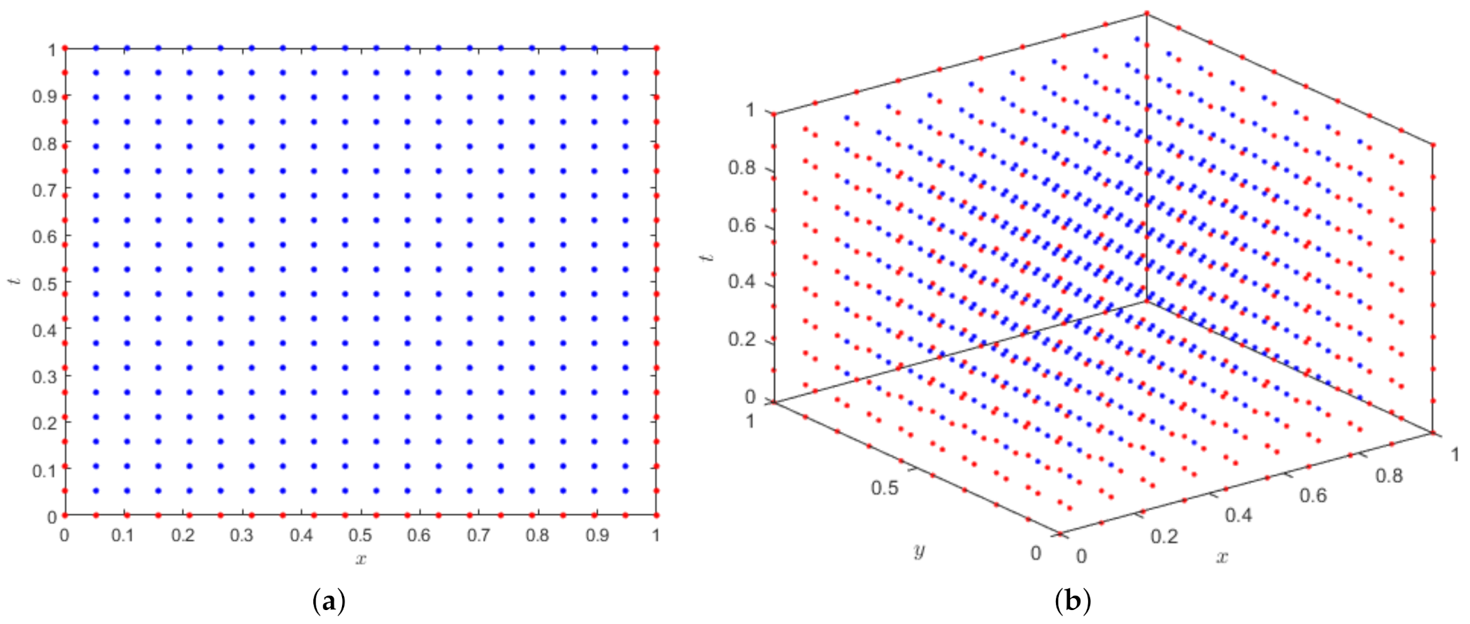
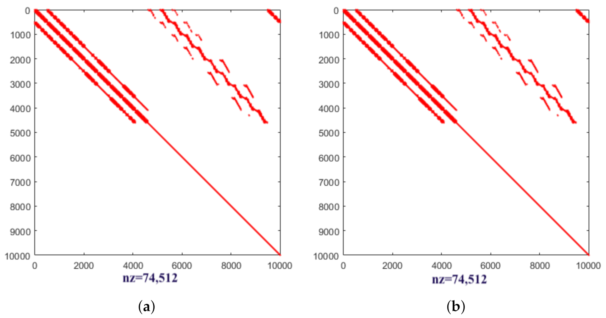
Figure 1.
Data location scheme for (a) Example 1 and (b) Example 2.
Figure 1.
Data location scheme for (a) Example 1 and (b) Example 2.
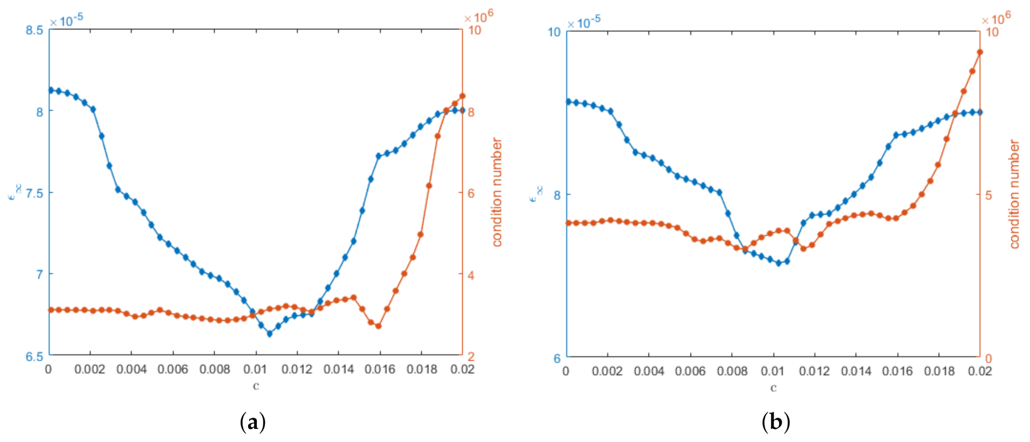
Figure 2.
Absolute errors and condition numbers for Example 1 by letting and for different shape parameter c with respect to (a) wave model and (b) damped wave model.
Figure 2.
Absolute errors and condition numbers for Example 1 by letting and for different shape parameter c with respect to (a) wave model and (b) damped wave model.
Figure 3.
Absolute errors for Example 1 by letting , , and for different time level t (a) ; (b) and (c) with respect to wave model.
Figure 3.
Absolute errors for Example 1 by letting , , and for different time level t (a) ; (b) and (c) with respect to wave model.
Figure 4.
Absolute errors for Example 1 by letting , , and for different time level t (a) ; (b) and (c) with respect to damped wave model.
Figure 4.
Absolute errors for Example 1 by letting , , and for different time level t (a) ; (b) and (c) with respect to damped wave model.
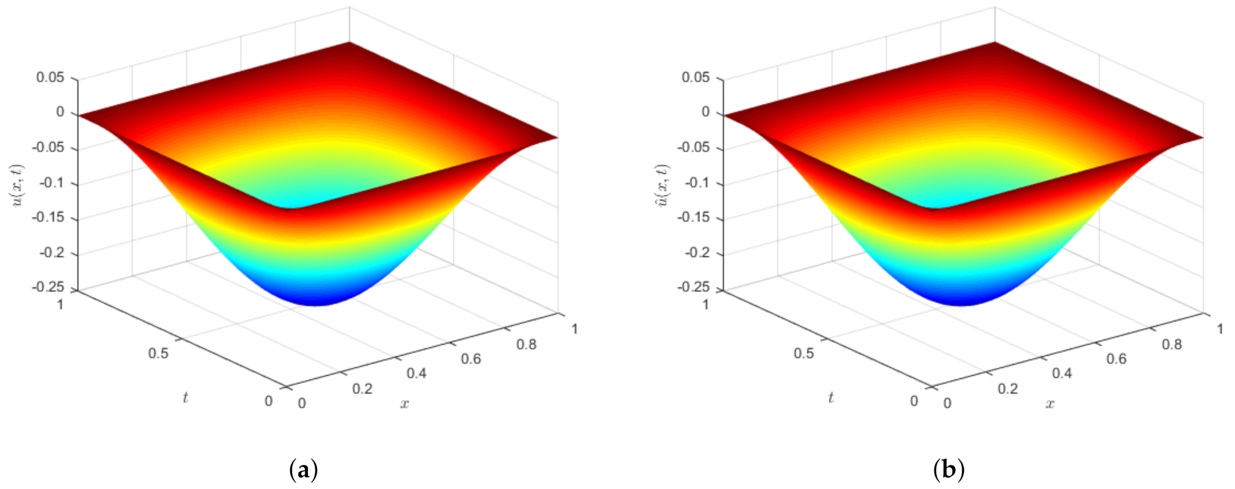
Figure 5.
The plots of (a) exact solution and (b) approximation solution for Example 1 by taking , , and with respect to wave model.
Figure 5.
The plots of (a) exact solution and (b) approximation solution for Example 1 by taking , , and with respect to wave model.
Figure 6.
The plots of (a) exact solution and (b) approximation solution for Example 1 by taking , , and with respect to damped wave model.
Figure 6.
The plots of (a) exact solution and (b) approximation solution for Example 1 by taking , , and with respect to damped wave model.
Figure 7.
The sparsity pattern of the coefficient matrix for Example 1 with respect to (a) wave model (b) damped wave model.
Figure 7.
The sparsity pattern of the coefficient matrix for Example 1 with respect to (a) wave model (b) damped wave model.
Figure 8.
The sparsity pattern of the coefficient matrix for Example 2 with respect to (a) wave model (b) damped wave model.
Figure 8.
The sparsity pattern of the coefficient matrix for Example 2 with respect to (a) wave model (b) damped wave model.
Figure 9.
Absolute errors and condition numbers for Example 2 by letting and for different shape parameter c with respect to (a) wave model and (b) damped wave model.
Figure 9.
Absolute errors and condition numbers for Example 2 by letting and for different shape parameter c with respect to (a) wave model and (b) damped wave model.
Figure 10.
Absolute errors for Example 2 by letting , , , and for different time level t (a) ; (b) and (c) with respect to wave model.
Figure 10.
Absolute errors for Example 2 by letting , , , and for different time level t (a) ; (b) and (c) with respect to wave model.
Figure 11.
Absolute errors for Example 2 by letting , , , and different time level t (a) ; (b) and (c) with respect to damped wave model.
Figure 11.
Absolute errors for Example 2 by letting , , , and different time level t (a) ; (b) and (c) with respect to damped wave model.
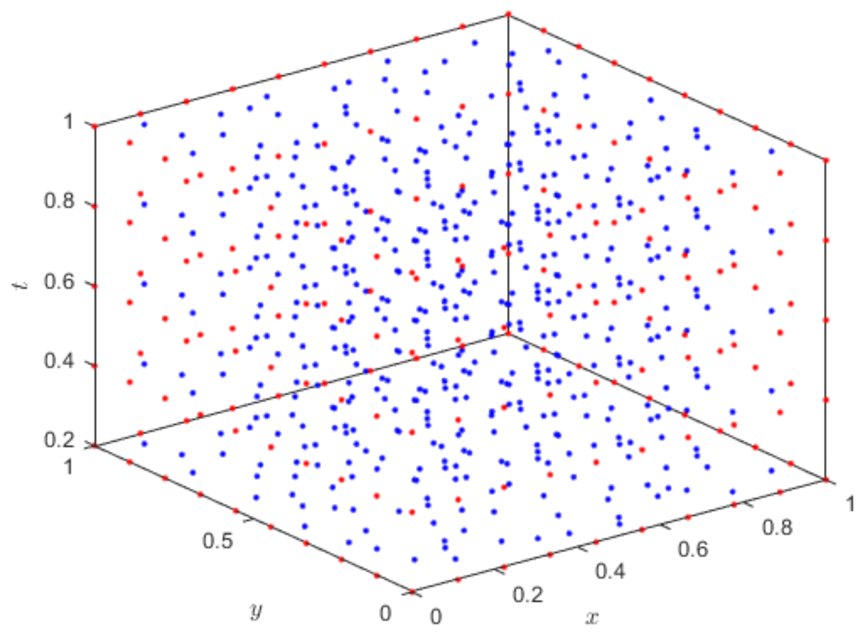
Figure 12.
Data location scheme for Example 3 with irregular distribution.
Figure 12.
Data location scheme for Example 3 with irregular distribution.
Figure 13.
The absolute errors vs. the number of data points for Example 3 with respect to (a) wave model (b) damped wave model.
Figure 13.
The absolute errors vs. the number of data points for Example 3 with respect to (a) wave model (b) damped wave model.
Figure 14.
The condition numbers vs. the number of data points for Example 3 with respect to (a) wave model (b) damped wave model.
Figure 14.
The condition numbers vs. the number of data points for Example 3 with respect to (a) wave model (b) damped wave model.
Figure 15.
The sparsity pattern of the coefficient matrix for Example 3 with respect to wave model with (a) uniform distribution of points (b) irregular distribution of points.
Figure 15.
The sparsity pattern of the coefficient matrix for Example 3 with respect to wave model with (a) uniform distribution of points (b) irregular distribution of points.
Figure 16.
The sparsity pattern of the coefficient matrix for Example 3 with respect to damped wave model with (a) uniform distribution of points (b) irregular distribution of points.
Figure 16.
The sparsity pattern of the coefficient matrix for Example 3 with respect to damped wave model with (a) uniform distribution of points (b) irregular distribution of points.
Figure 17.
Absolute errors and condition numbers for Example 4 by letting and for different shape parameter c with respect to (a) wave model and (b) damped wave model.
Figure 17.
Absolute errors and condition numbers for Example 4 by letting and for different shape parameter c with respect to (a) wave model and (b) damped wave model.
Figure 18.
The sparsity pattern of the coefficient matrix for Example 4 with respect to (a) wave model (b) damped wave model.
Figure 18.
The sparsity pattern of the coefficient matrix for Example 4 with respect to (a) wave model (b) damped wave model.
Table 1.
Error estimates, condition numbers, CPU times and convergence rate of Example 1 by letting and different values of N and several fractional orders .
Table 1.
Error estimates, condition numbers, CPU times and convergence rate of Example 1 by letting and different values of N and several fractional orders .
| N | Wave Model | | Damped Wave Model |
|---|
| c | | | | Time | | | c | | | | Time | |
|---|
| | 0.006 | | | | | − | | 0.006 | | | | | − |
| | | 0.007 | | | | | | | 0.007 | | | | | |
| | | 0.008 | | | | | | | 0.008 | | | | | |
| | | 0.009 | | | | | | | 0.009 | | | | | |
| | | 0.010 | | | | | | | 0.010 | | | | | |
| | | 0.015 | | | | | | | 0.012 | | | | | |
| | 0.006 | | | | | − | | 0.006 | | | | | − |
| | | 0.007 | | | | | | | 0.007 | | | | | |
| | | 0.008 | | | | | | | 0.008 | | | | | |
| | | 0.009 | | | | | | | 0.009 | | | | | |
| | | 0.010 | | | | | | | 0.010 | | | | | |
| | | 0.015 | | | | | | | 0.012 | | | | | |
| | 0.006 | | | | | − | | 0.005 | | | | | − |
| | | 0.007 | | | | | | | 0.006 | | | | | |
| | | 0.008 | | | | | | | 0.007 | | | | | |
| | | 0.009 | | | | | | | 0.008 | | | | | |
| | | 0.010 | | | | | | | 0.009 | | | | | |
| | | 0.015 | | | | | | | 0.010 | | | | | |
Table 2.
Error estimates for of Example 1 by letting in wave model and in damped wave model, , different values of and several fractional orders .
Table 2.
Error estimates for of Example 1 by letting in wave model and in damped wave model, , different values of and several fractional orders .
| | Wave Model | | Damped Wave Model |
|---|
| | | | |
|---|
| 15 | | | | | |
| | 20 | | | | | |
| | 25 | | | | | |
| | 30 | | | | | |
| 15 | | | | | |
| | 20 | | | | | |
| | 25 | | | | | |
| | 30 | | | | | |
| 15 | | | | | |
| | 20 | | | | | |
| | 25 | | | | | |
| | 30 | | | | | |
Table 3.
The effect of noise on error estimates of Example 1 for different values of N and letting .
Table 3.
The effect of noise on error estimates of Example 1 for different values of N and letting .
| N | | Wave Model | | Damped Wave Model |
|---|
| | | | | | |
|---|
| 0 | | | | | | | |
| | | | | | | | | |
| | | | | | | | | |
| | | | | | | | | |
| 0 | | | | | | | |
| | | | | | | | | |
| | | | | | | | | |
| | | | | | | | | |
| 0 | | | | | | | |
| | | | | | | | | |
| | | | | | | | | |
| | | | | | | | | |
| 0 | | | | | | | |
| | | | | | | | | |
| | | | | | | | | |
| | | | | | | | | |
Table 4.
The effect of noise on error estimates of Example 4 for different values of N and letting , and .
Table 4.
The effect of noise on error estimates of Example 4 for different values of N and letting , and .
| N | | Wave Model | | Damped Wave Model |
|---|
| | | | | | |
|---|
| 0 | | | | | | | |
| | | | | | | | | |
| | | | | | | | | |
| | | | | | | | | |
| 0 | | | | | | | |
| | | | | | | | | |
| | | | | | | | | |
| | | | | | | | | |
| 0 | | | | | | | |
| | | | | | | | | |
| | | | | | | | | |
| | | | | | | | | |
| 0 | | | | | | | |
| | | | | | | | | |
| | | | | | | | | |
| | | | | | | | | |
Table 5.
Error estimates, condition numbers, CPU times convergence rate of Example 2 by letting and different values of N and several fractional orders and .
Table 5.
Error estimates, condition numbers, CPU times convergence rate of Example 2 by letting and different values of N and several fractional orders and .
| N | Wave Model | | Damped Wave Model |
|---|
| c | | | | Time | | | c | | | | Time | |
|---|
| | 0.006 | | | | | − | | 0.008 | | | | | − |
| | | 0.009 | | | | | | | 0.009 | | | | | |
| | | 0.011 | | | | | | | 0.011 | | | | | |
| | | 0.016 | | | | | | | 0.016 | | | | | |
| | 0.008 | | | | | − | | 0.009 | | | | | − |
| | | 0.010 | | | | | | | 0.010 | | | | | |
| | | 0.013 | | | | | | | 0.013 | | | | | |
| | | 0.020 | | | | | | | 0.020 | | | | | |
| | 0.008 | | | | | − | | 0.009 | | | | | − |
| | | 0.010 | | | | | | | 0.010 | | | | | |
| | | 0.013 | | | | | | | 0.013 | | | | | |
| | | 0.020 | | | | | | | 0.020 | | | | | |
Table 6.
Error estimates for of Example 2 by letting for wave model and for damped wave model, , different values of and several fractional orders and .
Table 6.
Error estimates for of Example 2 by letting for wave model and for damped wave model, , different values of and several fractional orders and .
| | Wave Model | | Damped Wave Model |
|---|
| | | | |
|---|
| 5 | | | | | |
| | 10 | | | | | |
| | 15 | | | | | |
| | 20 | | | | | |
| 5 | | | | | |
| | 10 | | | | | |
| | 15 | | | | | |
| | 20 | | | | | |
| 5 | | | | | |
| | 10 | | | | | |
| | 15 | | | | | |
| | 20 | | | | | |
Table 7.
The effect of noise on error estimates of Example 2 for different values of N and letting and .
Table 7.
The effect of noise on error estimates of Example 2 for different values of N and letting and .
| N | | Wave Model | | Damped Wave Model |
|---|
| | | | | | |
|---|
| 0 | | | | | | | |
| | | | | | | | | |
| | | | | | | | | |
| | | | | | | | | |
| 0 | | | | | | | |
| | | | | | | | | |
| | | | | | | | | |
| | | | | | | | | |
| 0 | | | | | | | |
| | | | | | | | | |
| | | | | | | | | |
| | | | | | | | | |
| 0 | | | | | | | |
| | | | | | | | | |
| | | | | | | | | |
| | | | | | | | | |
Table 8.
Error estimates, condition numbers, CPU times and convergence rate of Example 4 by letting and different values of N and several fractional orders , , .
Table 8.
Error estimates, condition numbers, CPU times and convergence rate of Example 4 by letting and different values of N and several fractional orders , , .
| N | Wave Model | | Damped Wave Model |
|---|
| c | | | | Time | | | c | | | | Time | |
|---|
| | 0.030 | | | | | − | | 0.009 | | | | | − |
| | | 0.035 | | | | | | | 0.011 | | | | | |
| | | 0.074 | | | | | | | 0.014 | | | | | |
| | | 0.099 | | | | | | | 0.019 | | | | | |
| | 0.030 | | | | | − | | 0.010 | | | | | − |
| | | 0.037 | | | | | | | 0.014 | | | | | |
| | | 0.041 | | | | | | | 0.017 | | | | | |
| | | 0.050 | | | | | | | 0.020 | | | | | |
| | 0.020 | | | | | − | | 0.011 | | | | | − |
| | | 0.030 | | | | | | | 0.015 | | | | | |
| | | 0.035 | | | | | | | 0.018 | | | | | |
| | | 0.035 | | | | | | | 0.021 | | | | | |
Table 9.
Error estimates for of Example 4 by letting for wave model and , , different values of and several fractional orders , , .
Table 9.
Error estimates for of Example 4 by letting for wave model and , , different values of and several fractional orders , , .
| | Wave Model | | Damped Wave Model |
|---|
| | | | |
|---|
| 3 | | | | | |
| | 6 | | | | | |
| | 9 | | | | | |
| | 12 | | | | | |
| 3 | | | | | |
| | 6 | | | | | |
| | 9 | | | | | |
| | 12 | | | | | |
| 3 | | | | | |
| | 6 | | | | | |
| | 9 | | | | | |
| | 12 | | | | | |


