Article

Dynamical Analysis and Finite-Time Synchronization for a Chaotic System with Hidden Attractor and Surface Equilibrium

1
Xi’an Key Laboratory of Human-Machine Integration and Control Technology for Intelligent Rehabilitation, School of Computer Science, Xijing University, Xi’an 710123, China
2
Shaanxi International Joint Research Center for Applied Technology of Controllable Neutron Source, School of Electronic Information, Xijing University, Xi’an 710123, China
*
Author to whom correspondence should be addressed.
Axioms 2022, 11(11), 579; https://doi.org/10.3390/axioms11110579
Submission received: 28 September 2022 / Revised: 17 October 2022 / Accepted: 20 October 2022 / Published: 22 October 2022
(This article belongs to the Special Issue Advances in Theory and Applications of Chaotic and Nonlinear Dynamics)

Abstract

:
In this paper, a chaotic system with surface equilibrium and a hidden attractor was studied, and the dynamical behavior, synchronization scheme and circuit application of the system were analyzed. Firstly, the stability analysis and dynamic behavior of the system were carried out (the type of attractor, bifurcation, Poincaré section, Lyapunov exponents spectrum and complexity). Secondly, the finite-time synchronization observer was designed according to the finite-time stability theorem to achieve the synchronization of the finite-time master–slave systems, and the error system asymptotically approached zero. Finally, the existence and practicability of the original system were proven through the implementation of the circuit system, and through using an appropriate control circuit to realize the synchronization of chaotic master–slave systems.

1. Introduction

Simple nonlinear differential equation systems can exhibit chaos, which is a universal phenomenon in nonlinear systems, and there is a large amount of evidence that chaos exists in reality [1]. In 1963, while designing a 3D model of atmospheric convection, Lorenz constructed a 3D quadratic polynomial ODE system in which he discovered the first chaotic attractor [2]. Later, many Lorenz-like systems, such as Sprott [3], Chen [4] and Lü [5], were constructed and studied, and studies of these systems also inspire us to think deeply about Lorenz-like systems. After Leonov put forward the mathematical definition of a hidden attractor [6], the research theory and application of a hidden attractor have been widely concerned [7], where the attraction domain does not intersect with the neighborhood of any unstable equilibria, and the basis of attraction is small for such systems [8,9]. Chaos cannot be excited by arbitrarily choosing the initial conditions near the unstable equilibria. Hence, the occurrence of hidden attractors in the system is not obvious and is difficult to be noticed [9]. Recently, chaotic systems with various equilibria have also been considered under the category of hidden attractors [10]; this includes systems with only one stable equilibrium [11,12], without an equilibrium [13,14] and with infinite equilibria [15,16,17]. There is a significant correlation between hidden attractors and multistability, which is a very important phenomenon in dynamic systems [18,19]. In fact, it is difficult to discover hidden attractors in physical systems as the systems themselves have specific physical properties that cannot be arbitrarily changed [20]. Meanwhile, hidden attractors are potentially harmful to engineering. Therefore, finding hidden attractors and identifying the dynamics of these system is challenging work. Moreover, chaotic systems with hidden attractors may have richer complex behavior than the self-excited attractors, so it is more helpful for the application of electronic circuits, artificial intelligence and so on [21,22,23].
The synchronization control of chaotic systems is also a classical and major topic of discussion in the field of nonlinear control [24,25,26]. For the actual chaotic systems, there are often some characteristics, such as various disturbances and uncertainties in the system, and the chaotic phenomenon is extremely sensitive to the initial value and parameter variation. Hence, using control strategies to achieve the synchronization control of uncertain chaotic systems with unknown parameters is still a challenge for some engineering applications, and this research is still an important and difficult problem to be urgently solved. For the uncertain chaotic synchronization control problem with unknown parameters, the dynamics and robustness of the master chaotic system following the slave chaotic system are key to measuring the synchronization performance. Aiming at this goal, researchers have proposed and verified many control methods: adaptive feedback synchronization control [27,28,29,30], sliding mode variable structure control [31,32,33] and robust control [34]. With the deepening of theoretical research, the methods of control are tending to maturity. Therefore, the research trend of chaotic synchronization will be how to realize the synchronization of chaotic systems with a simple structure, small control amount and finite time. Finite-time synchronization technology was first proposed by Haimo [35]. Yu [36] and Amato [37] proposed the concept of global robust terminal sliding mode control for a single input single output (SISO) of an uncertain nonlinear system and presented the design method of the controller. Then, finite-time synchronization control was applied to various engineering fields, including chaotic systems [38,39,40]. However, the parameters of chaotic synchronization used in practical engineering are variable and unknown, so the assumption of the above methods tend to be idealized. Meanwhile, there are few studies on the finite-time synchronization of chaotic systems with hidden attractors. Only when the synchronization error of the system converges in finite time and the control has strong robustness can it have a more practical engineering value. Thus, for the unique mechanism of chaotic systems with hidden attractors, the design of finite-time observers provide inspiration for solving the problems of sudden oscillations caused by hidden attractors. In this paper, we further elaborate on a chaotic system with surface equilibrium and a hidden attractor [41]:
x ˙ 1 = x 1 x 2 2 + a x 1 2 x 2 x ˙ 2 = x 1 x 3 x ˙ 3 = b x 1 + x 1 2 x 2
where x 1 , x 2 and x 3 are state variables of the system and a and b are parameters of the system. In this paper, the structure is as follows: in Section 2, the dynamical behavior of a chaotic system is analyzed, such as equilibria analysis, periodic orbit, Poincaré map, Lyapunov exponents spectrum (LEs), largest Lyapunov exponent (LLE), bifurcation diagram and complexity. In Section 3, the design method of the controller and law is presented to realize the finite-time robust feedback control of system (1). In Section 4, the circuit schematic diagram of the system (1) is given, and, by using an appropriate control circuit to realize the synchronization of master–slave systems, the reliability and existence of system (1) is verified by numerical simulation. The last section summarizes the dynamic analysis, control and circuit implementation, and gives prospects of future work.

2. Dynamical Properties

2.1. Equilibria and Stability

Let x ˙ 1 = 0 , x ˙ 2 = 0 , x ˙ 3 = 0 , its equilibria be S 1 b a , a b , 0 , S 2 b a , a b , 0 , S 3 ( 0 , x 2 , x 3 ) and its Jacobian matrix be
J = x 2 2 + 2 a x 1 x 2 2 x 1 x 2 + a x 1 2 0 x 3 0 x 1 b + 2 x 1 x 2 x 1 2 0
Let | λ E J | = 0 , and obtain its characteristic equation as
f ( λ ) = λ 3 + A 2 λ 2 + A 1 λ + A 0
From Equation (3),
A 2 = x 2 2 2 a x 1 x 2
A 1 = x 1 2 + a x 1 2 x 3 + 2 x 1 x 2 x 3
A 0 = x 1 2 x 2 2 2 a x 1 3 x 2 + 2 b x 1 2 x 2 + a b x 1 3 + 4 x 1 3 x 2 2 + 2 a x 1 4 x 2
According to Routh–Hurwitz criterion, when A 2 > 0 , A 0 > 0 and A 2 A 1 A 0 > 0 , the equilibrium is stable and is a stable point or stable point intersection; when A 2 > 0 , A 0 > 0 and A 2 A 1 A 0 < 0 , the equilibrium point is a saddle.

2.2. Dynamical Behaviors Analysis

In system (1), x 1 , x 2 and x 3 are state variables, and a and b are parameters. The dynamic characteristics of the system (1) depend on the variation in parameters a and b. When the parameters are set as a = 1.92 and b = 1 , and the initial state x 1 , x 2 , x 3 = 0.87 , 0.4 , 0 , the system (1) shows chaos, and the phase orbit diagram is shown in Figure 1.
In order to study the dynamics of system (1), a numerical simulation is used and Table 1 shows the various phase diagrams of system (1) under different parameters.

2.2.1. Phase Orbits

The phase diagrams with periodic-1, periodic-2 and chaos can be obtained when the parameter b = 1 is fixed and the parameter a is taken as 0.35, 0.95 and 1.92, respectively, as shown in Figure 2.

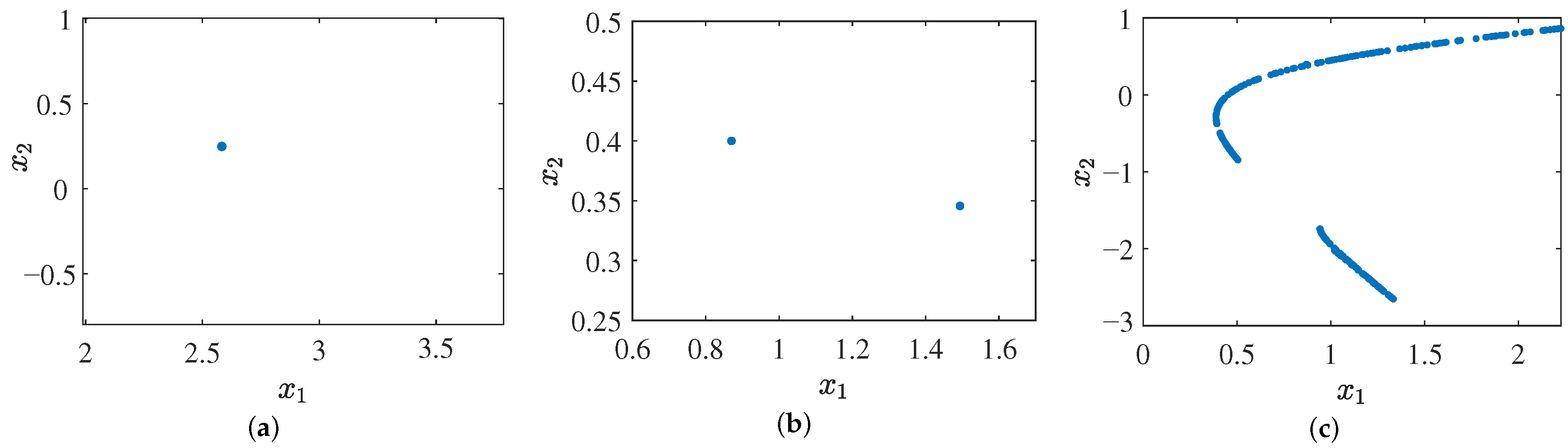
2.2.2. Poincaré Section

The Poincaré section is used to take fixed values for the conjugate variables and intercept a plane in multiple dimensions. As shown in Figure 3, when the parameter a is chosen to be 0.35, 0.95 and 1.92, respectively, and the fixed parameter b = 1 , the Poincaré section is in periodic-1, periodic-2 and chaos states in turn.
From Figure 3, when parameter a is set to 0.35 or 0.95, the Poincaré region will only have one or two discrete points, indicating periodic behavior of the system (1), and, as the parameter a is set to 1.92, the Poincaré section is continuous with dense points, indicating that the system (1) exhibits chaos.

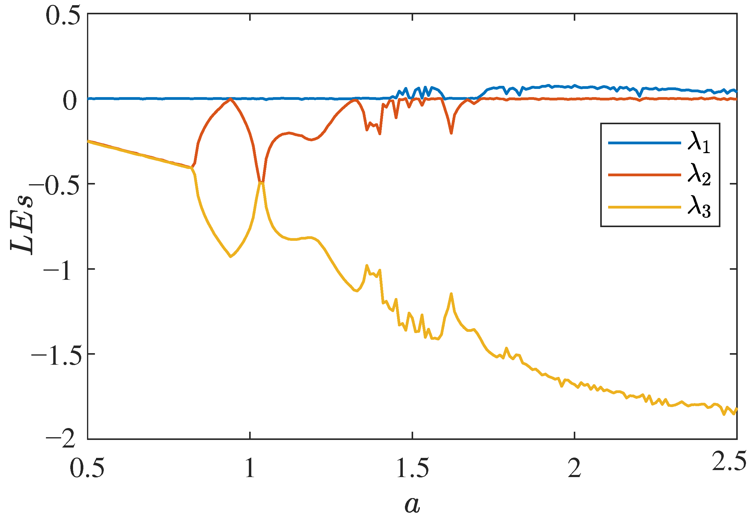
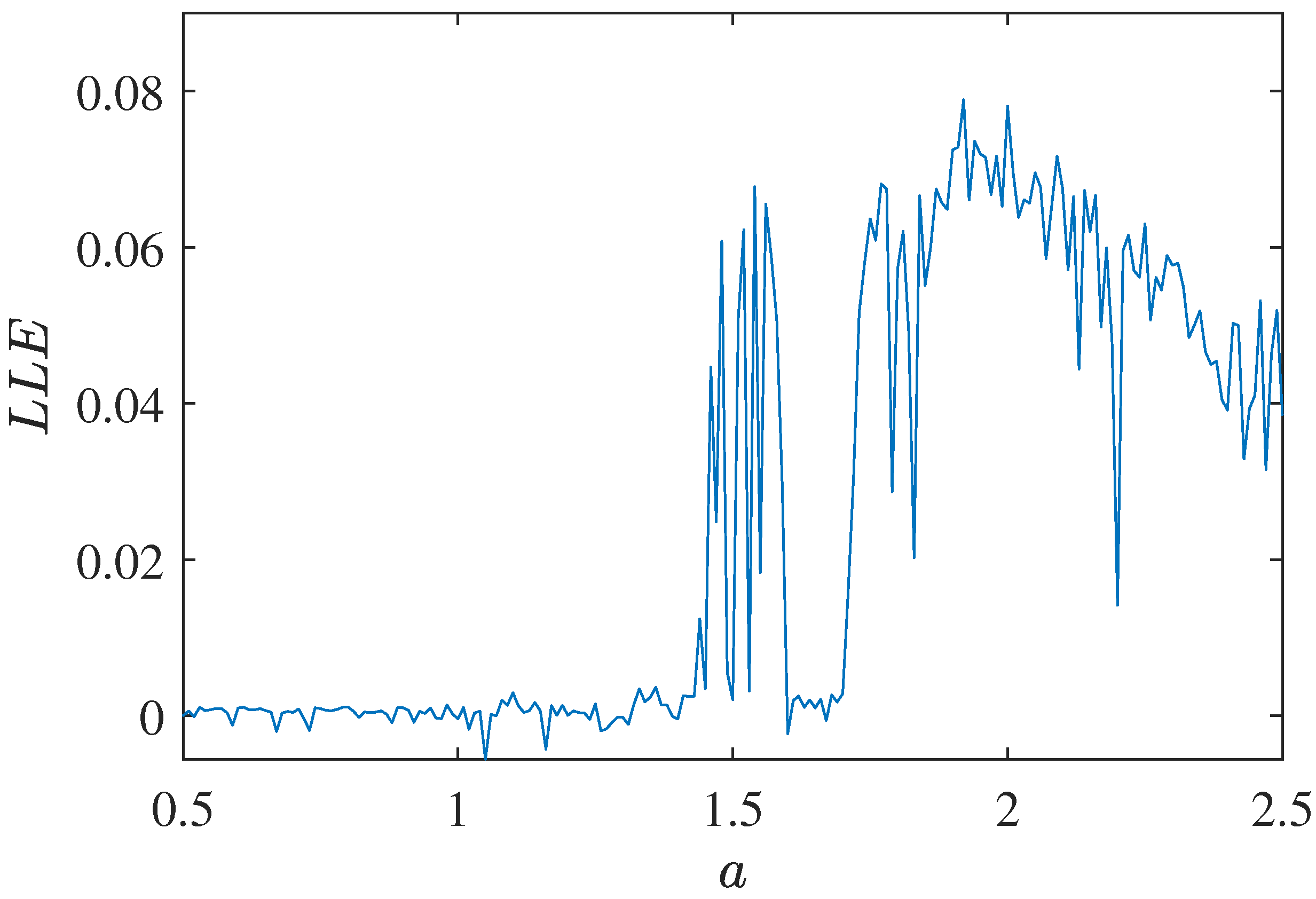
2.2.3. Lyapunov Exponent
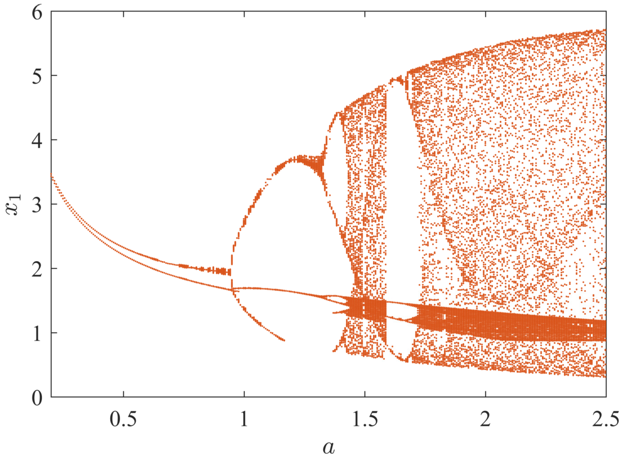
For system (1), the Lyapunov dimension can be used to characterize the geometric properties of chaotic attractors. Its defining equation is:
D λ = j + 1 λ j + 1 i = 1 j λ i
The above equation has a system dimension of D λ = 2.040 for a = 1.92 and b = 1 , and the system (1) has a fractal Lyapunov dimension, which shows the chaotic state. In order to confirm it, we need to fix the parameter b, change the parameter a and calculate the Lyapunov exponents spectrum of the system (1). The Lyapunov exponent spectrum of system (1) shown in Figure 4 fluctuates in the interval 0.5 , 2.5 , whereas Figure 5 shows the largest Lyapunov exponent.
From Figure 5, the largest Lyapunov exponent λ 1 > 0 is observed. This observation is also confirmed in Table 1.

2.2.4. Bifurcation

A bifurcation diagram can also describe the chaotic states of system (1). Through the bifurcation state in Figure 6, the state of system (1) clearly changes from periodic to chaotic; then, combined with observing the Lyapunov exponents spectrum, it is found that system (1) changes its state when the parameter a changes, indicating that system (1) can only generate chaotic behavior within a certain parameter range.
According to the diagram above, parameter a can determine whether system (1) is in a chaotic state or periodic state. The complex dynamic behavior of system (1) can be controlled more easily by changing the value of a.

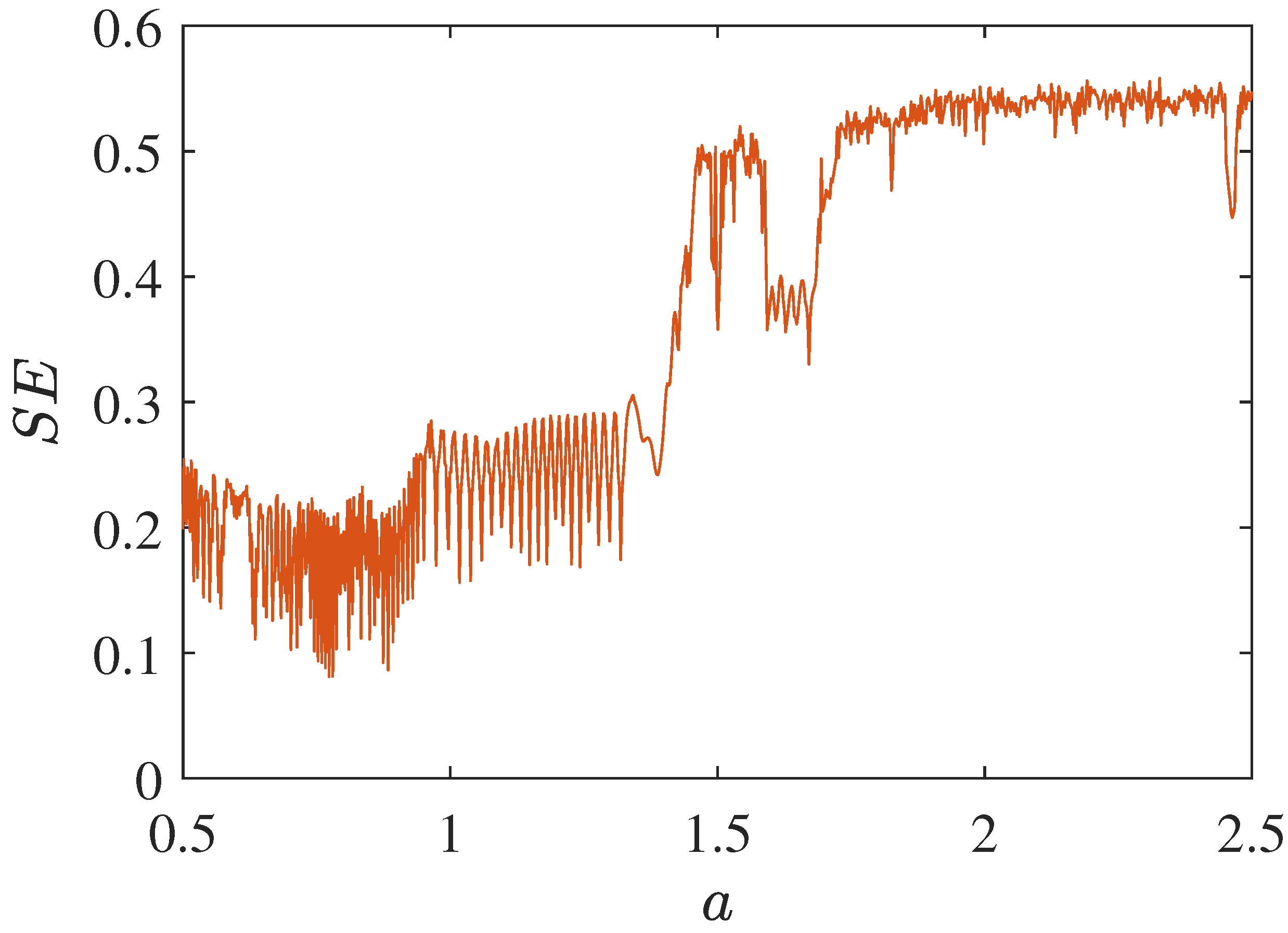
2.2.5. Complexity Resolution

The complexity of system (1) is a measure of how similar a chaotic sequence is to a random sequence. The larger the complexity, the closer the sequence is to a random sequence. The spectral entropy complexity S E and complexity C 0 with parameter a for b = 1 are described in Figure 7 and Figure 8, respectively.
The analysis of the complexity S E and the complexity C 0 show that they are consistent with the Lyapunov exponents spectrum and the bifurcation diagram.

3. Design of Feedback Controller

3.1. Implementation of Robust Controller

The master system of system (1) can be expressed as follows:
x ˙ 1 = x 1 x 2 2 + a + Δ 1 x 1 2 x 2 x ˙ 2 = x 1 x 3 x ˙ 3 = b + Δ 2 x 1 + x 1 2 x 2
where x = x 1 , x 2 , x 3 T is the state variable of the master system, and the slave system can be defined as
y ˙ 1 = y 1 y 2 2 + a + Δ 3 y 1 2 y 2 + u 1 ( t ) y ˙ 2 = y 1 y 3 + u 2 ( t ) y ˙ 3 = b + Δ 4 y 1 + y 1 2 y 2 + u 3 ( t )
where y = y 1 , y 2 , y 3 T is the state variable of the slave system; Δ i i = 1 , 2 , 3 , 4 is the parameter uncertainty of the master–slave chaotic system; u i t = i = 1 , 2 , 3 is the external input controller.
Define the master–slave error as e i = y i x i i = 1 , 2 , 3 ; through calculation, the error system is
e ˙ 1 = e 1 y 2 2 1 + a y 1 + x 1 + x 1 e 2 y 2 + x 2 + a x 1 + Δ 3 e 1 y 1 2 + Δ 1 e 1 x 1 2 + u 1 ( t ) e ˙ 2 = e 1 y 3 x 1 e 3 + u 2 ( t ) e ˙ 3 = b x 2 y 1 + x 1 e 1 + y 2 2 e 2 + Δ 4 e 3 + Δ 2 e 3 + u 3 ( t )
Then, the robust feedback controller can be designed as
u 1 ( t ) = e 1 y 2 2 1 + a y 1 + x 1 x 1 e 2 y 2 + x 2 + a x 1 δ 3 e 1 y 1 2 δ 1 e 1 x 1 2 k e 1 ξ 1 s i g n e 1 u 2 ( t ) = e 1 y 3 + x 1 e 3 k e 2 ξ 2 s i g n e 2 u 3 ( t ) = b x 2 y 1 x 1 e 1 y 2 2 e 2 δ 4 e 3 δ 2 e 3 k e 3 ξ 3 s i g n e 3
where 0 < ξ i < 1   ( i = 1 , 2 , 3 ) and k > 0 . To facilitate the computational discussion, the following lemmas and assumption are required.
Lemma 1
([42]). When α, β and ξ are all positive and 0 < ξ < 1 , then we have the inequality α + β ξ α ξ + β ξ .
Lemma 2
([42]). (Finite time stability) If continuous, positive definite V t satisfies
V ˙ ( t ) ε V a ( t ) , t t 0 , V t 0 0
Among them, ε > 0 and 0 < a < 1 ; then, for any given t 0 , V t satisfies the following differential inequality:
V 1 a ( t ) V 1 a t 0 ε ( 1 a ) t t 0 , t 0 t t f i n
and, when t t f i n , there are V t = 0 ; among them, t f i n = t 0 + V 1 a t 0 ε 1 a .
Suppose that there exists a positive number δ i   i = 1 , 2 , 3 ; make the parameter perturbation Δ i δ i   i = 1 , 2 , 3 .

3.2. Performance of Robust Feedback Controller

After constructing systems (5) and (6) using the robust feedback controller (8), we have the following theorem:
Theorem 1.
For system (5) and system (6), the controller (8) is used, and 0 < ξ i < 1   i = 1 , 2 , 3 . Through Lemma 2, the finite-time T = t 0 + 2 σ 1 V σ t 0 σ , and then master–slave systems tend to be synchronized, where σ = 1 ξ 2 .
Proof. 
Construct the Lyapunov function V t = 1 2 i = 1 3 e i 2 , on the derivation of time t; V ˙ t = i = 1 3 e i . e ˙ i is available.
Substituting the three error systems (7) into the above equation, we can obtain
V ˙ ( t ) = e 1 e ˙ 1 + e 2 e ˙ 2 + e 3 e ˙ 3 = e 1 e 1 y 2 2 1 + a y 1 + x 1 + x 1 e 2 y 2 + x 2 + a x 1 + e 1 Δ 3 e 1 y 1 2 + Δ 1 e 1 x 1 2 + u 1 ( t ) + e 2 e 1 y 3 x 1 e 3 + u 2 ( t ) + e 3 b x 2 y 1 + x 1 e 1 + e 3 y 2 2 e 2 + Δ 4 e 3 + Δ 2 e 3 + u 3 ( t )
The robust feedback controller (8) is substituted into the above Equation (11), and terms are cancelled, to obtain
V ˙ ( t ) = e 1 Δ 3 e 1 y 1 2 + Δ 1 e 1 x 1 2 + e 1 δ 3 e 1 y 1 2 δ 1 e 1 x 1 2 k e 1 ξ 1 s i g n e 1 + e 2 k e 2 ξ 2 s i g n e 2 + e 3 δ 4 e 3 δ 2 e 3 k e 3 ξ 3 s i g n e 3 + e 3 Δ 4 e 3 + Δ 2 e 3
and, then, one can further obtain:
V ˙ ( t ) = Δ 3 e 1 2 y 1 2 δ 3 e 1 2 y 1 2 + Δ 1 e 1 2 x 1 2 δ 1 e 1 2 x 1 2 + Δ 4 e 3 2 δ 4 e 3 2 + Δ 2 e 3 2 δ 2 e 3 2 k e 1 ξ 1 e 1 k e 2 ξ 2 e 2 k e 3 ξ 3 e 3 = e 1 2 y 1 2 Δ 3 δ 3 + e 1 2 x 1 2 Δ 1 δ 1 + e 3 2 Δ 4 δ 4 + e 3 2 Δ 2 δ 2 k e 1 ξ 1 e 1 k e 2 ξ 2 e 2 k e 3 ξ 3 e 3
From Assumption 1, from the existence of positive numbers δ i   ( i = 1 , 2 , 3 ) , Δ i δ i   ( i = 1 , 2 , 3 . . . ) ,
e 1 2 y 1 2 Δ 3 δ 3 + e 1 2 x 1 2 Δ 1 δ 1 + e 3 2 Δ 4 δ 4 + e 3 2 Δ 2 δ 2 0
According to ξ , we have V ˙ t k e 1 ξ + 1 k e 2 ξ + 1 k e 3 ξ + 1 .
Combined with Lemma 1, we have
k e 1 ξ + 1 k e 2 ξ + 1 k e 3 ξ + 1 = 2 ξ + 1 2 k e 1 2 2 ξ + 1 2 + e 2 2 2 ξ + 1 2 + e 3 2 2 ξ + 1 2 2 ξ + 1 2 k e 1 2 2 + e 2 2 2 + e 3 2 2 ξ + 1 2
It is clear that V ˙ t 2 ξ + 1 2 k V ξ + 1 2 t .
From Lemma 2, it is known that there exists
T = t 0 + V 1 ξ + 1 2 t 0 2 ξ + 1 2 K 1 ξ + 1 2 = t 0 + 2 1 ξ 2 k V 1 ξ 2 t 0 1 ξ
and let σ = 1 ξ / 2 ; at finite time T = t 0 + 2 σ 1 V t 0 σ , the system containing parameter uncertainty achieves finite-time synchronization, where e i 0 i = 1 , 2 , 3 at t T . This completes the proof. □

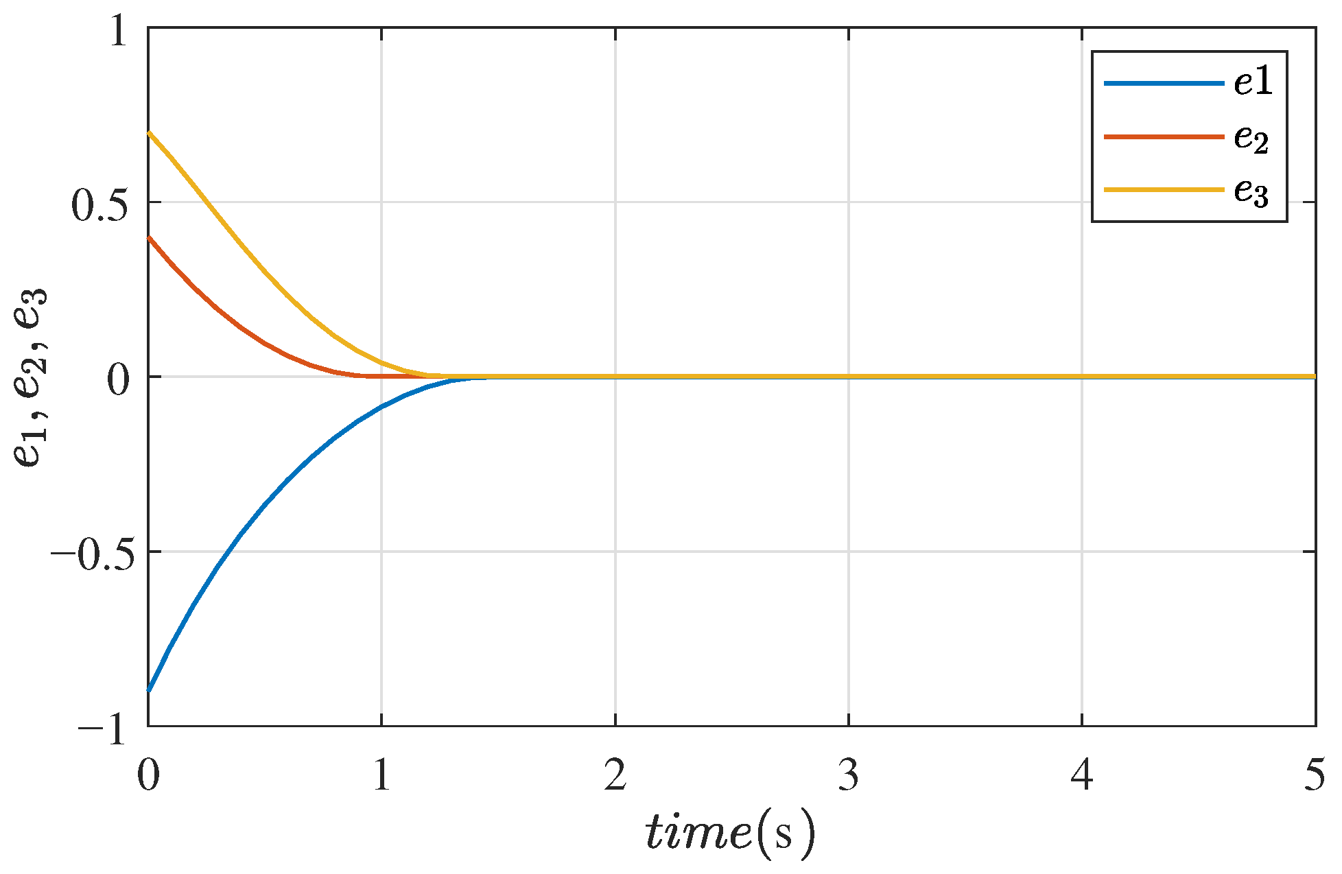
3.3. Numerical Simulation

For a master–slave system with parameters a = 1.92 , b = 1 and Δ i = 0 i = 1 , 2 , 3 , 4 , the system is in a chaotic state. The master–slave system applies a system controller with parameters taken as Δ 1 = 0.08 sin t , Δ 2 = 0.08 sin t , Δ 3 = 0.08 sin t and Δ 4 = 0.08 sin t ; then, it is known that δ 1 = 1 , δ 2 = 1 and δ 3 = 1 , δ 4 = 1 . The control parameters are taken as ξ 1 = 0.5 , ξ 2 = 0.5 and ξ 3 = 0.5 , and the orbits of the states of the master and slave systems are shown in Figure 9.
From Figure 9, the states of the master–slave system tend to converge, and synchronization errors are demonstrated in Figure 10.
From the simulation result in Figure 10, it can be seen that the trajectory of the synchronization error system converges asymptotically to the origin. In addition, Figure 9 and Figure 10 illustrate the control effect of the designed controller.

4. Circuit Implementation and Numerical Simulation

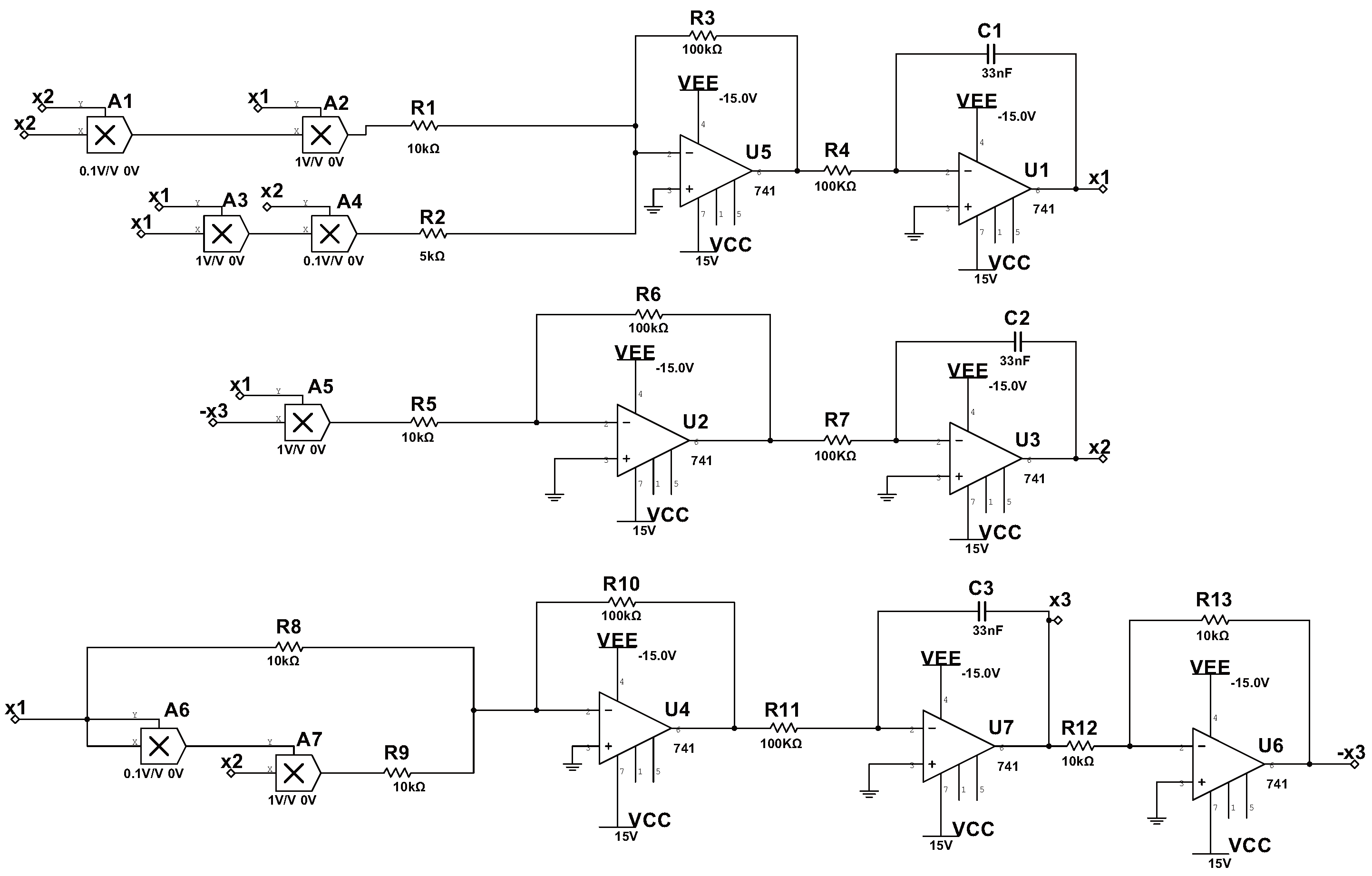
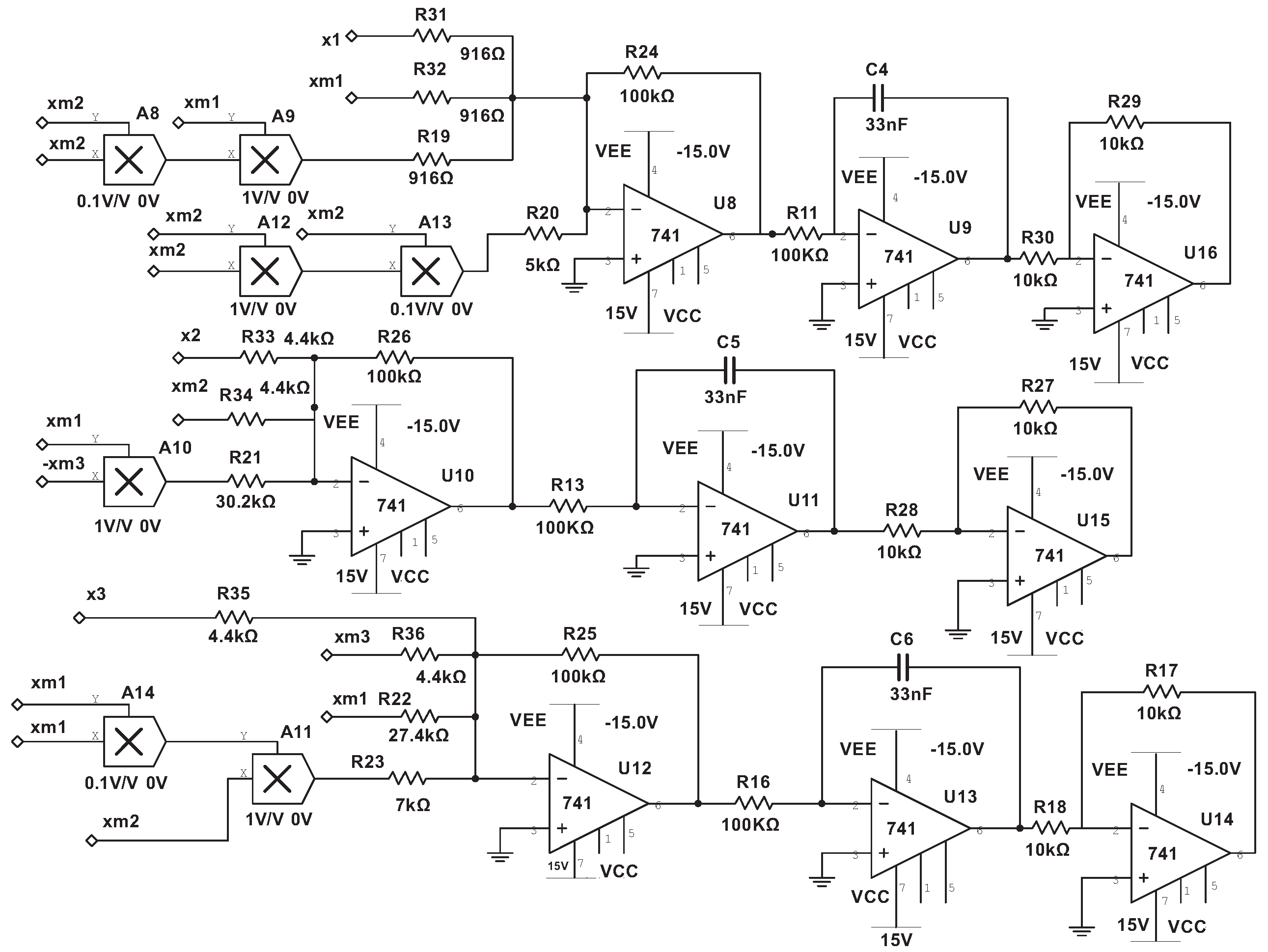
4.1. Circuit Implementation

We used the operational amplifier LM741, analog multiplier AD633, resistors and capacitors to design the analog circuit. The power voltage of the operational amplifier LM741 is ± 15 V, and its output saturation voltage is V s a t ± 13.5 V. According to system (5), a chaotic circuit was designed, as shown in Figure 11.
From Figure 11, applying Kirchhoff’s law, the corresponding circuit equations can be listed as
d x 1 d t = R 3 R 1 1 c 1 R 4 x 1 x 2 2 + R 3 R 2 1 c 1 R 4 x 2 x 1 2 d x 2 d t = R 6 R 5 1 c 2 R 7 x 1 x 3 d x 3 d t = R 14 R 15 R 10 R 8 1 c 3 R 12 x 1 + R 14 R 15 R 10 R 9 1 c 3 R 12 x 2 x 1 2
where x 1 , x 2 and x 3 are related to the voltage on the capacitors, respectively.

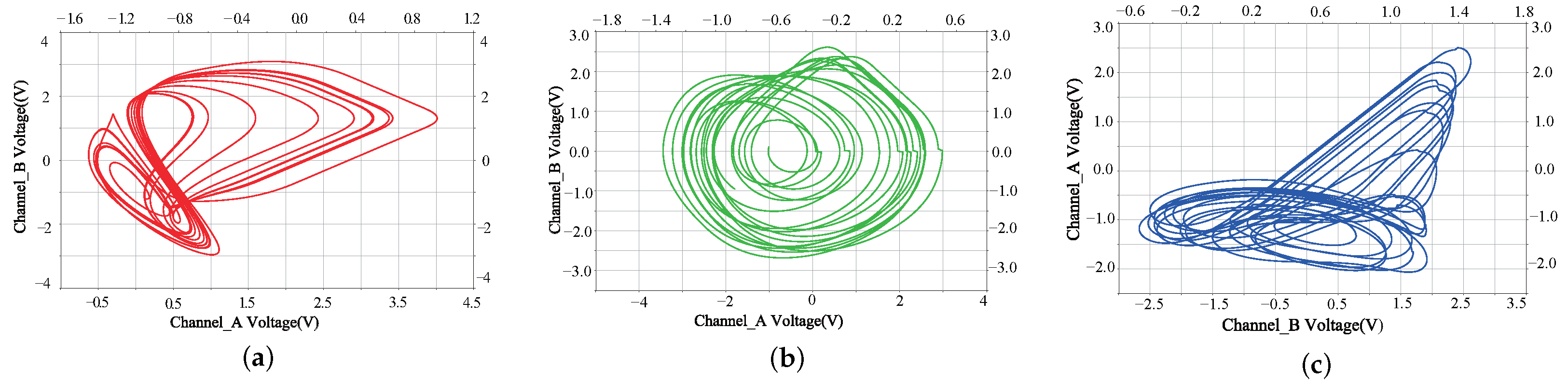
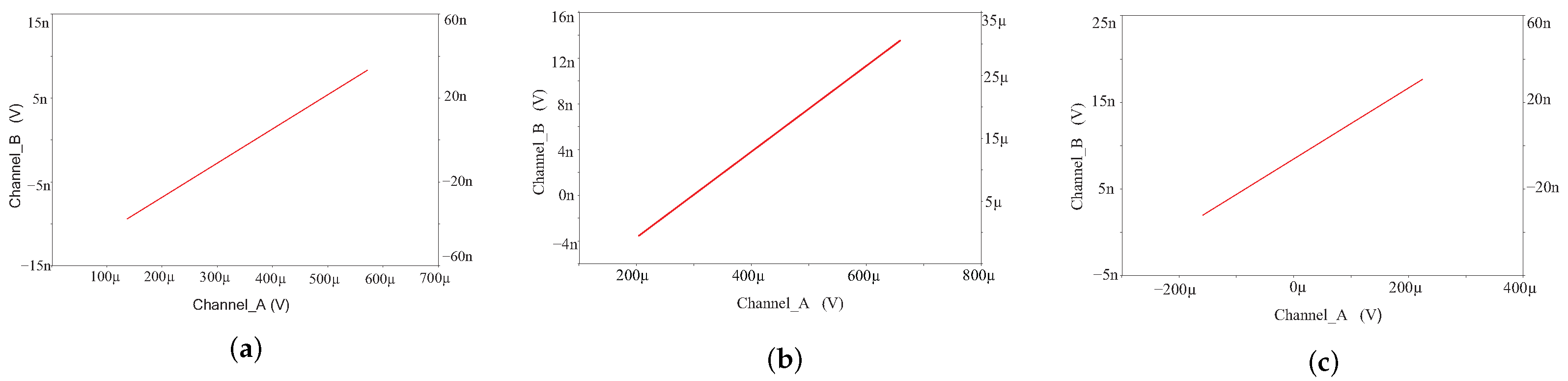
4.2. Circuit Simulation

For circuit system (17), capacitor C 1 = C 2 = C 3 = 33 nf, resistance R 2 = 5 k Ω , R 1 = R 5 = R 8 = R 9 = R 12 = R 13 = 10 k Ω , R 3 = R 4 = R 6 = R 7 = R 10 = R 11 = 100 k Ω can be obtained. The gain in the AD633 multiplier A 1 = A 4 = A 6 = 0.1 and A 2 = A 3 = A 5 = A 7 = 1 . According to the above circuit parameters, the phase diagram shown in Figure 12 can be obtained on a digital oscilloscope.
These results are consistent with the results of the numerical simulation and analog circuit simulation, which proves that the digital circuit can verify the chaotic behavior of this system. These numerical simulations are performed to verify the correctness of the system (1).
After realizing the above circuit simulation, in order to further achieve a synchronous circuit, the master system selects the chaotic system proposed in this paper, and system (1) can be rewritten as follows:
x ˙ m 1 = x 1 x 2 2 + a x 1 2 x 2 k 1 x m 1 x 1 x ˙ m 2 = x 1 x 3 k 2 x m 2 x 2 x ˙ m 3 = b x 1 + x 1 2 x 2 k 3 x m 3 x 3
where the parameters of the drive system are a = 1.92 , b = 1 , k 1 = 1 , k 2 = 22 and k 3 = 22 . The state vector is x = x m 1 , x m 2 , x m 3 T . The schematic diagram of the synchronization circuit and synchronization phase diagram are shown in Figure 13 and Figure 14. In addition, from Figure 14, it can be seen from the three phase planes that the master–slave system can achieve synchronization.

5. Conclusions

In this paper, we analyzedthe dynamical behavior of a surface equilibrium system with a hidden attractor (including phase analysis, Lyapunov exponent, bifurcation, Poincaré section, complexity, etc.). Moreover, a finite-time robust feedback controller was proposed for the synchronization and control problem of the surface equilibrium system with a hidden attractor, and the synchronization of master–slave systems in finite time was realized. Furthermore, a simulation circuit was designed to implement the system model, and the circuit synchronization simulation of the master–slave system was realized. The experimental results of the circuit are consistent with the simulation results of the theoretical model. Finally, in future work, we will find a better controller and implement its circuit, and a more comprehensive dynamic analysis of the system can also be carried out. By studying the latest results, the control method can also be further improved.

Author Contributions

Supervision, Z.W.; writing—visualization, H.T.; writing—original draft, R.Z.; writing—review and editing, X.X., H.T. and Z.W. All authors have read and agreed to the published version of the manuscript.

Funding

This work is supported by the National Natural Science Foundation of China (61973249), the Key Research and Development programs of Shaanxi Province (2021ZDLGY02-06), the Natural Science Basic Research Program of Shaanxi (2021JM-533, 2021JQ-880, 2020JM-646, 2021JQ-868), the Innovation Capability Support Program of Shaanxi (2018GHJD-21), the Qin Chuangyuan Project (2021QCYRC4-49), the Support Plan for Sanqin Scholars Innovation Team in Shaanxi Province of China, the National Defense Science and Technology Key Laboratory Fund Project (6142101210202), the Qinchuangyuan Scientist+Engineer (2022KXJ-169), the Scientific Research Program Funded by Shaanxi Provincial Education Department (21JK0960) and the Scientific Research Foundation of Xijing University (XJ210203).

Data Availability Statement

Not applicable.

Acknowledgments

The author acknowledges the referees and the editor for carefully reading this paper and giving many helpful comments. The authors also express their gratitude to the reviewers for their insightful comments.

Conflicts of Interest

The authors declare no conflict of interest.

References

  1. Kapitaniak, T.; Jafari, S. Nonlinear effects in life sciences. Eur. Phys. J. Spec. Top. 2018, 227, 693–696. [Google Scholar] [CrossRef] [Green Version]
  2. Lorenz, E.N. Deterministic nonperiodic flow. J. Atmos. Sci. 1963, 20, 130–141. [Google Scholar] [CrossRef]
  3. Sprott, J.C. Some simple chaotic flows. Phys. Rev. E 1994, 50, R647. [Google Scholar] [CrossRef] [PubMed]
  4. Chen, G.; Ueta, T. Yet another chaotic attractor. Int. J. Bifurc. Chaos 1999, 9, 1465–1466. [Google Scholar] [CrossRef]
  5. Lü, J.; Chen, G. A new chaotic attractor coined. Int. J. Bifurc. Chaos 2002, 12, 659–661. [Google Scholar] [CrossRef] [Green Version]
  6. Leonov, G.A.; Kuznetsov, N.V. Algorithms for Searching for Hidden Oscillations in the Aizerman and Kalman Problems; Springer: Berlin/Heidelberg, Germany, 2011. [Google Scholar]
  7. Tian, H.; Wang, Z.; Zhang, H.; Cao, Z.; Zhang, P. Dynamical analysis and fixed-time synchronization of a chaotic system with hidden attractor and a line equilibrium. Eur. Phys. J. Spec. Top. 2022, 231, 2455–2466. [Google Scholar] [CrossRef]
  8. Leonov, G.A.; Kuznetsov, N.V. Hidden attractors in dynamical systems. From hidden oscillations in Hilbert–Kolmogorov, Aizerman, and Kalman problems to hidden chaotic attractor in Chua circuits. Int. J. Bifurc. Chaos 2013, 23, 1330002. [Google Scholar] [CrossRef] [Green Version]
  9. Dudkowski, D.; Jafari, S.; Kapitaniak, T.; Kuznetsov, N.V.; Leonov, G.A.; Prasad, A. Hidden attractors in dynamical systems. Phys. Rep. 2016, 637, 1–50. [Google Scholar] [CrossRef]
  10. Wang, Z.; Wei, Z.; Sun, K.; He, S.; Wang, H.; Xu, Q.; Chen, M. Chaotic flows with special equilibria. Eur. Phys. J. Spec. Top. 2020, 229, 905–919. [Google Scholar] [CrossRef]
  11. Wang, X.; Chen, G. A chaotic system with only one stable equilibrium. Commun. Nonlinear Sci. Numer. Simul. 2012, 17, 1264–1272. [Google Scholar] [CrossRef]
  12. Deng, Q.; Wang, C.; Yang, L. Four-wing hidden attractors with one stable equilibrium point. Int. J. Bifurc. Chaos 2020, 30, 2050086. [Google Scholar] [CrossRef]
  13. Wei, Z. Dynamical behaviors of a chaotic system with no equilibria. Phys. Lett. A 2011, 376, 102–108. [Google Scholar] [CrossRef]
  14. Jafari, S.; Sprott, J.C.; Golpayegani, S.M.R.H. Elementary quadratic chaotic flows with no equilibria. Phys. Lett. A 2013, 377, 699–702. [Google Scholar] [CrossRef]
  15. Li, C.; Sprott, J.C.; Thio, W. Bistability in a hyperchaotic system with a line equilibrium. J. Exp. Theor. Phys. 2014, 118, 494–500. [Google Scholar] [CrossRef]
  16. Li, Q.; Hu, S.; Tang, S.; Zeng, G. Hyperchaos and horseshoe in a 4D memristive system with a line of equilibria and its implementation. Int. J. Circuit Theory Appl. 2014, 42, 1172–1188. [Google Scholar] [CrossRef]
  17. Kingni, S.T.; Pham, V.T.; Jafari, S.; Kol, G.R.; Woafo, P. Three-dimensional chaotic autonomous system with a circular equilibrium: Analysis, circuit implementation and its fractional-order form. Circuits, Syst. Signal Process. 2016, 35, 1933–1948. [Google Scholar] [CrossRef]
  18. Kapitaniak, T.; Leonov, G.A. Multistability: Uncovering hidden attractors. Eur. Phys. J. Spec. Top. 2015, 224, 1405–1408. [Google Scholar] [CrossRef] [Green Version]
  19. Wang, N.; Zhang, G.; Kuznetsov, N.V.; Bao, H. Hidden attractors and multistability in a modified Chua’s circuit. Commun. Nonlinear Sci. Numer. Simul. 2021, 92, 105494. [Google Scholar] [CrossRef]
  20. Yang, Y.; Qi, G.; Hu, J.; Faradja, P. Finding method and analysis of hidden chaotic attractors for plasma chaotic system from physical and mechanistic perspectives. Int. J. Bifurc. Chaos 2020, 30, 2050072. [Google Scholar] [CrossRef]
  21. Wang, Z.; Baruni, S.; Parastesh, F.; Jafari, S.; Ghosh, D.; Perc, M.; Hussain, I. Chimeras in an adaptive neuronal network with burst-timing-dependent plasticity. Neurocomputing 2020, 406, 117–126. [Google Scholar] [CrossRef]
  22. Wang, Z.; Parastesh, F.; Rajagopal, K.; Hamarash, I.I.; Hussain, I. Delay-induced synchronization in two coupled chaotic memristive Hopfield neural networks. Chaos Solitons Fractals 2020, 134, 109702. [Google Scholar] [CrossRef]
  23. Liang, H.; Wang, Z.; Yue, Z.; Lu, R. Generalized synchronization and control for incommensurate fractional unified chaotic system and applications in secure communication. Kybernetika 2012, 48, 190–205. [Google Scholar]
  24. Xi, X.; Mobayen, S.; Ren, H.; Jafari, S. Robust finite-time synchronization of a class of chaotic systems via adaptive global sliding mode control. J. Vib. Control 2018, 24, 3842–3854. [Google Scholar] [CrossRef]
  25. Ghosh, D. Nonlinear-observer–based synchronization scheme for multiparameter estimation. EPL (Europhys. Lett.) 2008, 84, 40012. [Google Scholar] [CrossRef]
  26. Chaudhary, H.; Khan, A.; Nigar, U.; Kaushik, S.; Sajid, M. An Effective Synchronization Approach to Stability Analysis for Chaotic Generalized Lotka–Volterra Biological Models Using Active and Parameter Identification Methods. Entropy 2022, 24, 529. [Google Scholar] [CrossRef]
  27. Sun, J.; Wang, Y.; Wang, Y.; Shen, Y. Finite-time synchronization between two complex-variable chaotic systems with unknown parameters via nonsingular terminal sliding mode control. Nonlinear Dyn. 2016, 85, 1105–1117. [Google Scholar] [CrossRef]
  28. Deng, Y.; Hu, H.; Xiong, W.; Xiong, N.N.; Liu, L. Analysis and design of digital chaotic systems with desirable performance via feedback control. IEEE Trans. Syst. Man Cybern. Syst. 2015, 45, 1187–1200. [Google Scholar] [CrossRef]
  29. Ghosh, D.; Banerjee, S. Adaptive scheme for synchronization-based multiparameter estimation from a single chaotic time series and its applications. Phys. Rev. E 2008, 78, 056211. [Google Scholar]
  30. Ghosh, D.; Frasca, M.; Rizzo, A.; Majhi, S.; Rakshit, S.; Alfaro-Bittner, K.; Boccaletti, S. The synchronized dynamics of time-varying networks. Phys. Rep. 2022, 949, 1–63. [Google Scholar] [CrossRef]
  31. Chen, W.; Zhang, R.; Zhao, L.; Wang, H.; Wei, Z. Control of chaos in vehicle lateral motion using the sliding mode variable structure control. Proc. Inst. Mech. Eng. Part J. Automob. Eng. 2019, 233, 776–789. [Google Scholar] [CrossRef]
  32. Wang, C.; Tang, J.; Jiang, B.; Wu, Z. Sliding-mode variable structure control for complex automatic systems: A survey. Math. Biosci. Eng. 2022, 19, 2616–2640. [Google Scholar] [CrossRef]
  33. Liu, J.; Wang, Z.; Chen, M.; Zhang, P.; Yang, R.; Yang, B. Chaotic system dynamics analysis and synchronization circuit realization of fractional-order memristor. Eur. Phys. J. Spec. Top. 2022, 1–13. [Google Scholar] [CrossRef]
  34. Tian, H.; Wang, Z.; Zhang, P.; Chen, M.; Wang, Y. Dynamic analysis and robust control of a chaotic system with hidden attractor. Complexity 2021, 2021, 8865522. [Google Scholar] [CrossRef]
  35. Haimo, V.T. Finite time controllers. SIAM J. Control Optim. 1986, 24, 760–770. [Google Scholar] [CrossRef]
  36. Yu, S.; Yu, X.; Zhihong, M. Robust global terminal sliding mode control of SISO nonlinear uncertain systems. In Proceedings of the 39th IEEE Conference on Decision and Control (Cat. No. 00CH37187), Sydney, Australia, 12–15 December 2000; IEEE: Piscataway, NJ, USA, 2000; Volume 3, pp. 2198–2203. [Google Scholar]
  37. Amato, F.; Ariola, M.; Dorato, P. Finite-time control of linear systems subject to parametric uncertainties and disturbances. Automatica 2001, 37, 1459–1463. [Google Scholar] [CrossRef]
  38. Li, S.; Tian, Y. Finite time synchronization of chaotic systems. Chaos Solitons Fractals 2003, 15, 303–310. [Google Scholar] [CrossRef]
  39. Perruquetti, W.; Floquet, T.; Moulay, E. Finite-time observers: Application to secure communication. IEEE Trans. Autom. Control 2008, 53, 356–360. [Google Scholar] [CrossRef] [Green Version]
  40. Wang, H.; Ye, J.; Miao, Z.; Jonckheere, E.A. Robust finite-time chaos synchronization of time-delay chaotic systems and its application in secure communication. Trans. Inst. Meas. Control 2018, 40, 1177–1187. [Google Scholar] [CrossRef]
  41. Jafari, S.; Sprott, J.C.; Pham, V.T.; Volos, C.; Li, C. Simple chaotic 3D flows with surfaces of equilibria. Nonlinear Dyn. 2016, 86, 1349–1358. [Google Scholar] [CrossRef]
  42. Aghababa, M.P.; Khanmohammadi, S.; Alizadeh, G. Finite-time synchronization of two different chaotic systems with unknown parameters via sliding mode technique. Appl. Math. Model. 2011, 35, 3080–3091. [Google Scholar] [CrossRef]
Figure 1. Chaos of system (1) with a = 1.92 , b = 1 .
Axioms 11 00579 g001
Figure 2. Periodic-1 and 2 and chaotic orbit of the system (1) with different a. (a) a = 0.35 , b = 1 . (b) a = 0.95 , b = 1 . (c) a = 1.92 , b = 1 . (d) a = 0.35 , b = 1 . (e) a = 0.95 , b = 1 . (f) a = 1.92 , b = 1 . (g) a = 0.35 , b = 1 . (h) a = 0.95 , b = 1 . (i) a = 1.92 , b = 1 .
Axioms 11 00579 g002
Figure 3. Periodic-1 and 2 and chaotic Poincaré surface of section of the system (1) with different a. (a) a = 0.35 , b = 1 . (b) a = 0.95 , b = 1 . (c) a = 1.92 , b = 1 .
Axioms 11 00579 g003
Figure 4. Lyapunov exponents spectrum (LEs) of the system (1) for b = 1 .
Axioms 11 00579 g004
Figure 5. Largest Lyapunov exponent (LLE) of the system (1) for b = 1 .
Axioms 11 00579 g005
Figure 6. Bifurcation of system (1) for b = 1 .
Axioms 11 00579 g006
Figure 7. Complexity S E of system (1).
Axioms 11 00579 g007
Figure 8. Complexity C 0 of system (1).
Axioms 11 00579 g008
Figure 9. Synchronization of master-slave system. (a) x 1 , y 1 . (b) x 2 , y 2 . (c) x 3 , y 3 .
Axioms 11 00579 g009
Figure 10. Time responses of the synchronization errors.
Axioms 11 00579 g010
Figure 11. Analog circuit of the system (1).
Axioms 11 00579 g011
Figure 12. Analog circuit simulation phase results of system (1). (a) x 1 x 2 . (b) x 2 x 3 . (c) x 3 x 1 .
Axioms 11 00579 g012
Figure 13. Schematic diagram of synchronization analog circuit of system (1).
Axioms 11 00579 g013
Figure 14. Analog circuit simulation results of system (1). (a) x 1 , x m 1 . (b) x 2 , x m 2 . (c) x 3 , x m 3 .
Axioms 11 00579 g014
Table 1. Dynamic behavior of the system (1) with different parameters (PVs, parameter values; PPs, phase portraits; Ps, Poincaré section).
PVsDynamicsLESPPsPs
a = 0.35 Periodic-1[0, −0.1728, −0.1786]Figure 2a,d,gFigure 3a
a = 0.95 Periodic-2[0, −0.0217, −0.1945]Figure 2b,e,hFigure 3b
a = 1.92 Chaotic[0.0661, 0, −1.664]Figure 2c,f,iFigure 3c
Publisher’s Note: MDPI stays neutral with regard to jurisdictional claims in published maps and institutional affiliations.

