1. Introduction
In the current literature, a large number of papers falsely claimed to have generalized the classical Laplace transform and the
s-multiplied (or the Laplace–Carson) transform by making some obviously trivial changes in the parameter
s and the argument
t. Most (if not all) of such trivialities and inconsequential variations of the classical Laplace transform and the Laplace–Carson transform, which appeared and continue to appear in the literature, were pointed out and documented by H. M. Srivastava (see [
1], pp. 1508–1510, and [
2], pp. 36–38).
In order not to create misunderstandings, we want to say right away that the purpose of this article is not to provide generalizations of the Laplace transform (LT), but only to extend the tables of LTs often used in applied mathematics. The well known tables of Oberhettinger and Badii cited among the references [
3] does not include the LT of functions considered in this paper.
We want to underline the fact that in literature it is usually considered that there are no formulas for the computation of the LT of composed functions. This belief has been refuted in a previous article [
4] and the possibility of obtaining approximations in this field is shown in an even more general situation in this paper. As far as we know, there are no other articles on this topic and our approach seems to be the first in this regard.
More precisely, we show how to approximate the Laplace transform of a 2-variable composed analytic function
, where
,
are analytic functions, by using the bivariate Bell polynomials, a suitable set of Bell polynomials, introduced in a preceding paper [
5].
The classical Bell polynomials are exploited in very different frameworks, which range from number theory [
6,
7,
8,
9,
10] to operators theory [
11,
12], and from differential equations [
13] to integral transforms [
14,
15]. Applications of the Laplace Transform (LT) in Analysis and Mathematical Physics problems are well known [
16].
We use the classical definition:
The LT converts a function of a real variable t (representing the time) to a function of a complex variable s (representing the complex frequency).
The LT can be applied to locally integrable functions on . It converges in each half plane , where a is a constant (called the convergence abscissa), depending on the growth behavior of .
Owing to the importance of this transformation in the solution of the most diverse differential problems, a large number of LT, together with the respective anti-transforms, are reported in literature (see, e.g., [
3,
17]).
Given a 2-variable composed function
it is natural to define the relevant LT by putting:
In previous articles, we have shown how to compute the LT of higher-order nested functions (see [
4] and the references therein). In this article, we apply a similar method to approximate the LT of a composed analytic function of 2 variables, taking advantage of the bivariate Bell polynomials introduced in [
5]. The results obtained demonstrate the correctness of the method considered, as can be seen in the numerical verifications obtained by the first author using the Mathematica
computer algebra system.
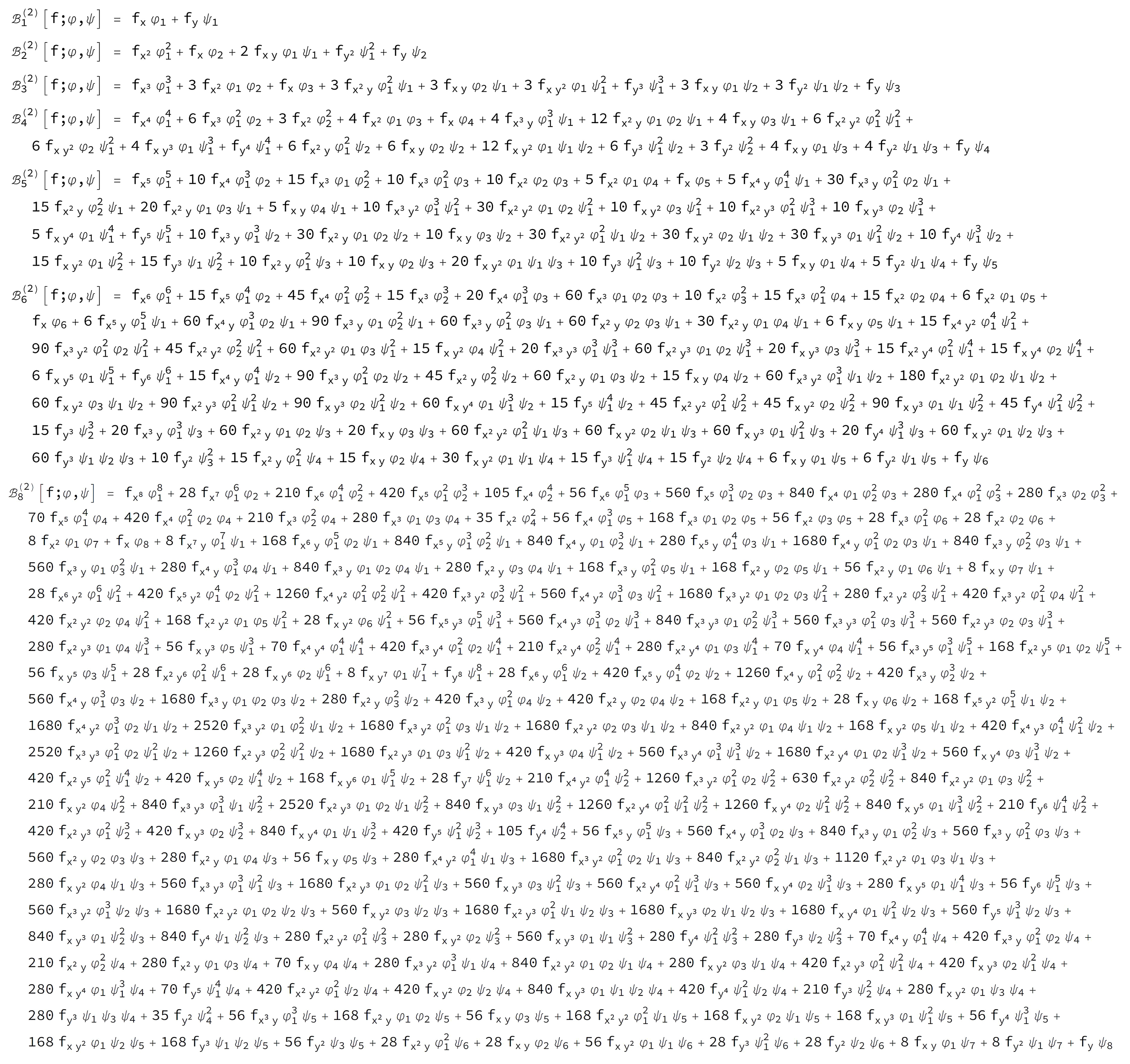
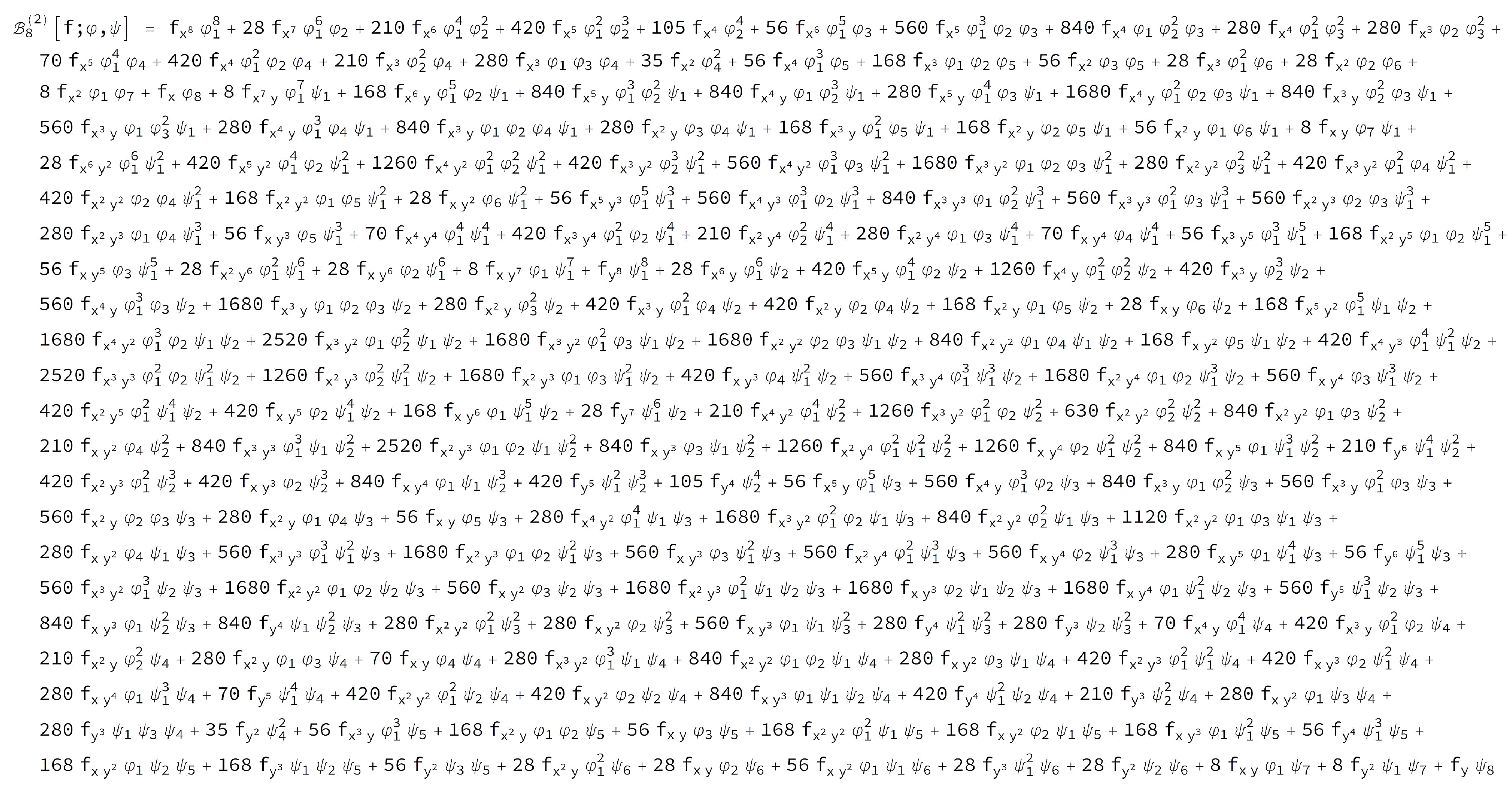
The first bivariate Bell polynomials are given in the
Appendix A at the end of this article.
2. Recalling the Bell’s Polynomials
The Bell’s polynomials [
18] express the
nth derivative of a composed function
in terms of the successive derivatives of the (sufficiently smooth) component functions
and
. More precisely, if
then the
nth derivative of
is represented by
where
denotes the
nth Bell polynomial.
The first few Bell polynomials are given by:
More general results can be found in [
19], p. 49.
The Bell polynomials [
6] are given by the equation
where the
satisfy the recursion [
6]
The functions for any are polynomials in the variables homogeneous of degree k and isobaric of weight n (i.e., they are linear combinations of monomials whose weight is constantly given by ).
Therefore, we have the equations
and
3. Bivariate Bell’s Polynomials
Consider the composed function under the standard assumptions on the domains of definition and differentiability. Compute the the partial derivative of the function f, h-times with respect to x and k-times with respect to y and then put . Indicate the result with , and also set , .
Hence, the bivariate Bell polynomials are defined as follows:
Note that
where
denotes the
nth ordinary Bell polynomial defined in (
1).
In the above formula, for the formal multiplication symbol ∘, we assume the definition below
Therefore, we find the result [
5].
Theorem 1. Let be analytical functions. The nth polynomial of the system , can be computed with the following rule By the Leibniz rule, we can write
Then, for the bivariate Bell polynomials, the recurrence relation holds
4. LT of a 2-Variable Composed Function
Let
be a composed function, analytic in a neighborhood of the origin, so that it is expressed by the Taylor’s expansion:
According to the preceding equations, it results
where
where
denotes the
kth derivative of the function
with respect to
t.
Using the previous formulas we are able to approximate the calculation of the LT of the function with that of a series of elementary LT of powers. In fact, we have the following Theorem.
Theorem 3. Considering a composed function , expressed by the Taylor’s expansion in Equation (
15)
, for its LT the following equation holdswhere the symbolic power in the above equation must be computed using the definitions in (
11).
Proof. Representing the coefficients of the Taylor expansion in (
15) in terms of bivariate Bell polynomials, and using the uniform convergence of series, we find
Then, the result follows from elementary calculation of the LT of powers. □
5. Examples
5.1. The Particular Case of Exponential Functions
We start considering the case of the nested exponential function
Example 1
Then,
, and for the relevant LT, using the above described method, we find
5.2. The General Case
Examples of the above method for approximating the LT of general nested functions are reported in what follows.
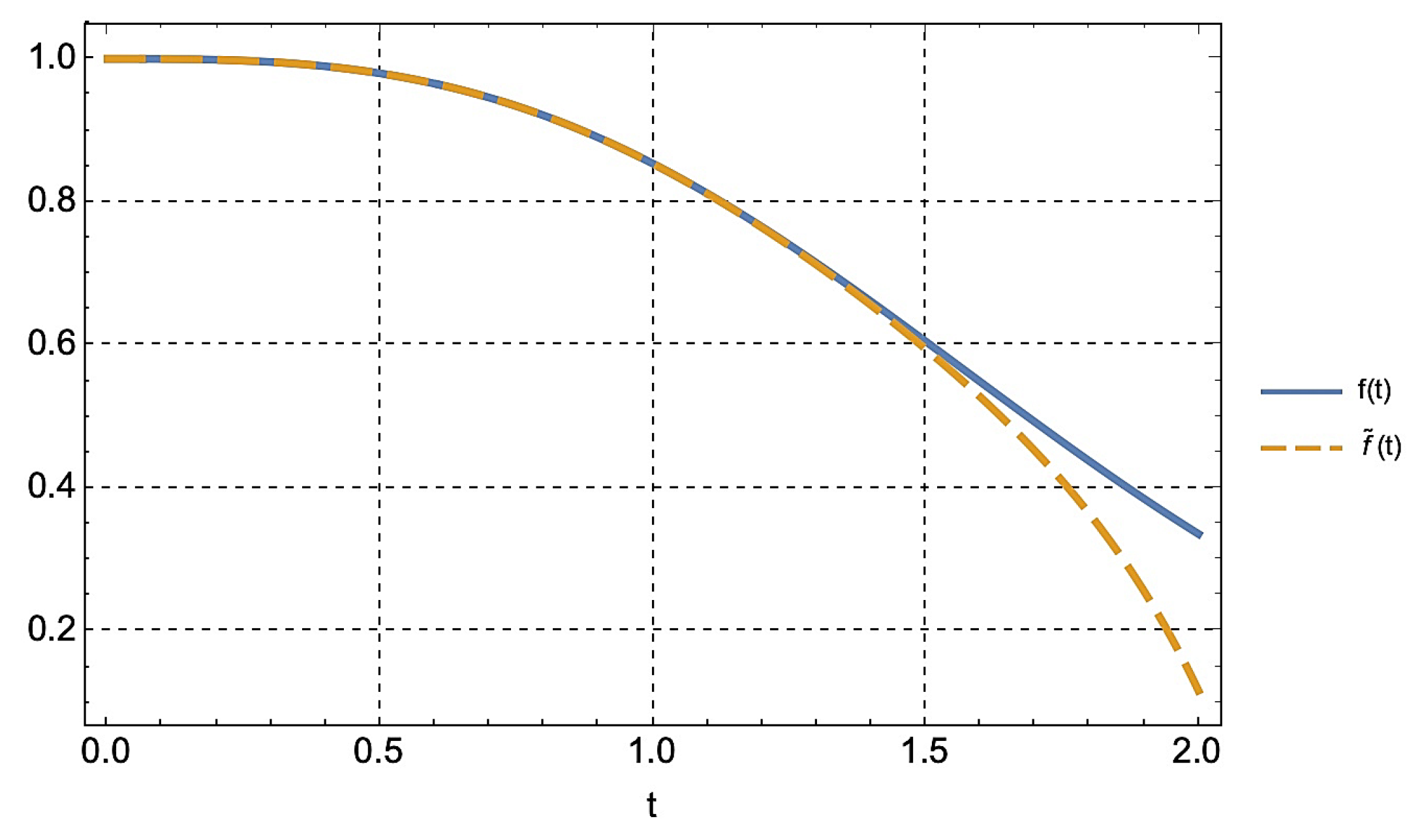
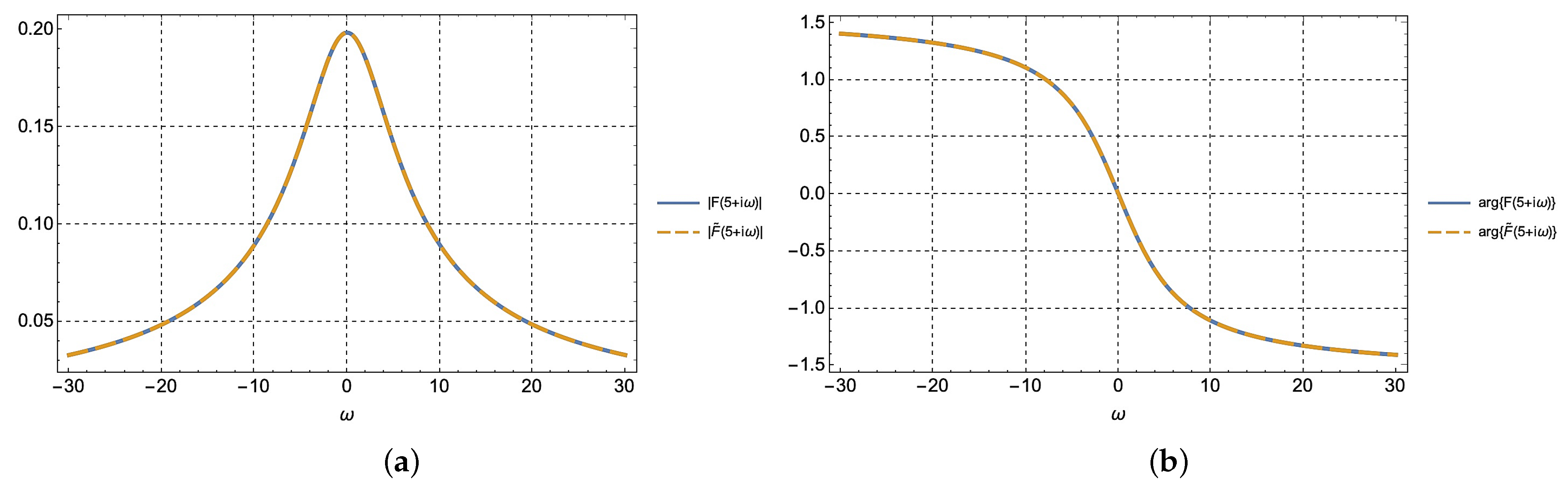
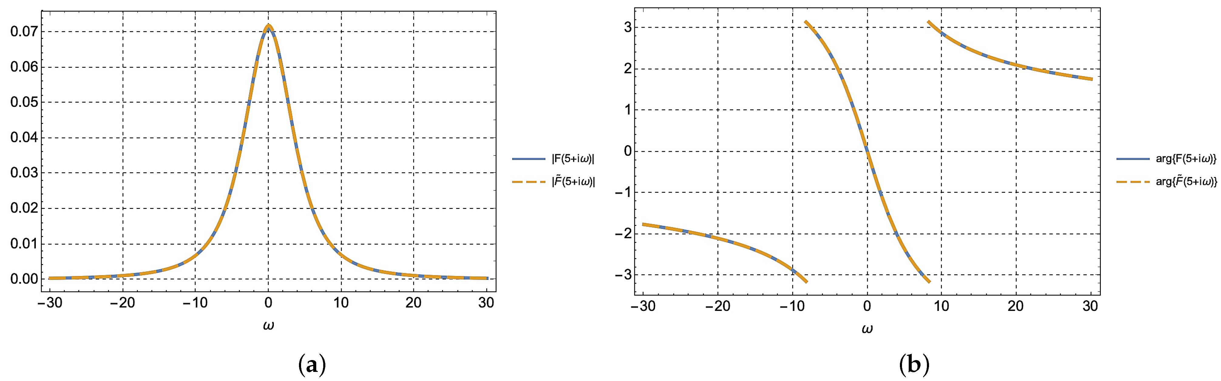
5.2.1. Example 2
Assuming , , we have . By using the above described method, for the relevant LT we find the approximation:
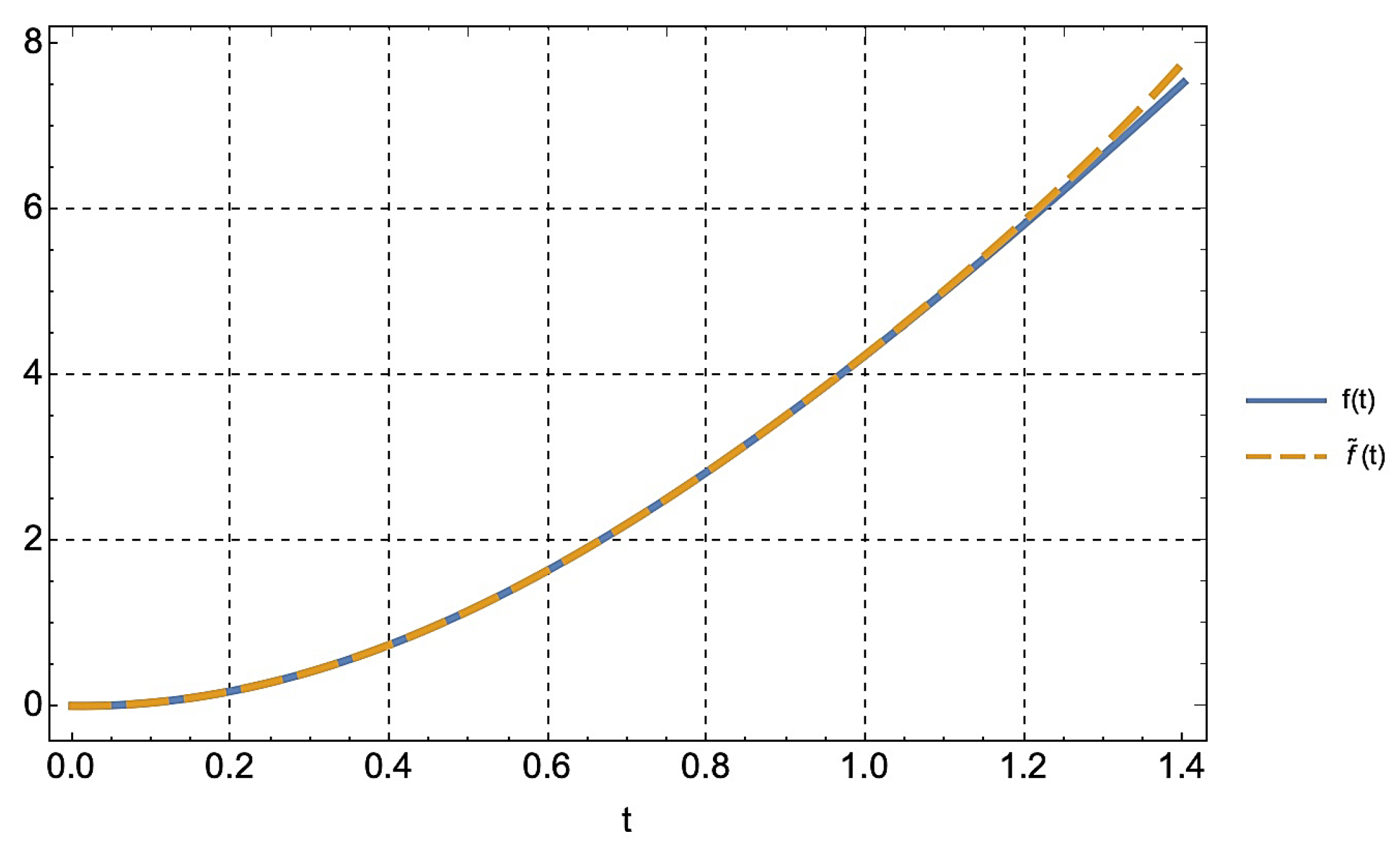
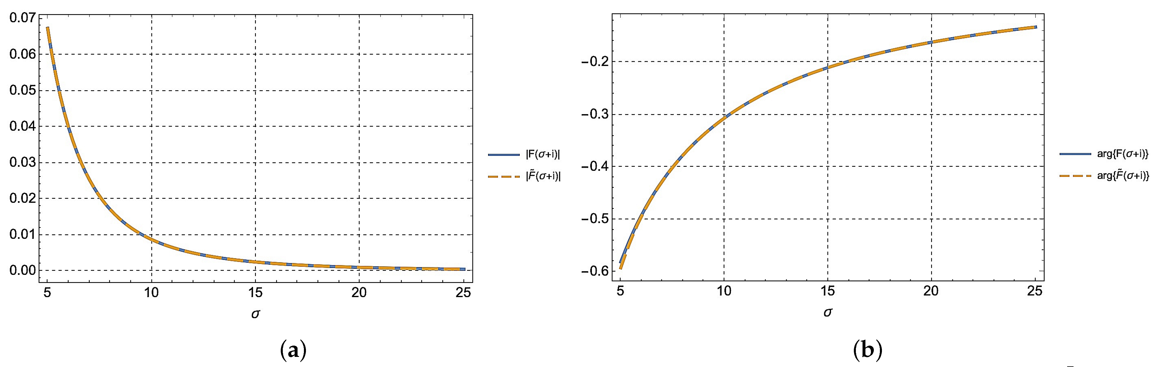
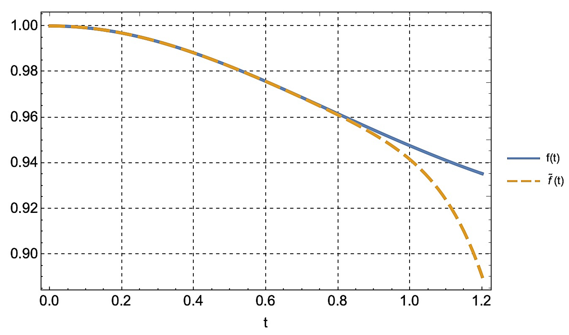
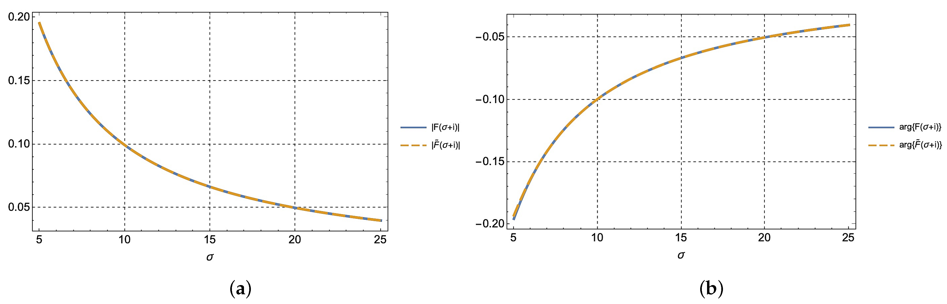
5.2.2. Example 3
Assuming , , we have . By using the above described method, for the relevant LT we find the approximation:
6. Conclusions
We have shown a method for approximating the LT of a 2-variable composed function , where , , are analytic functions, by using the bivariate Bell polynomials. Starting from the Taylor expansion in a neighborhood of the origin of the function , since the coefficients can be expressed in terms of the bivariate Bell polynomials, the integral is reduced to the computation of an approximating series, which obviously converges if the integral is convergent.
We, thus, showed that just as it was possible to approximate the LT of composed functions using Bell polynomials [
4], so it can be done for the LT of composed functions in two variables, using the bivariate Bell polynomials, introduced in [
5].
In the last section, the proposed technique is checked in some particular cases, when the transform and the anti-transform are known, proving the correctness of our results.
Extension could be made to higher nested functions by using the results in [
4].
Author Contributions
Conceptualization, D.C., R.S. and P.E.R.; methodology, D.C., R.S. and P.E.R.; software, D.C.; validation, D.C., R.S. and P.E.R.; investigation, D.C., R.S. and P.E.R.; data curation, D.C.; writing—original draft preparation, P.E.R.; visualization, D.C.; funding acquisition, R.S. All authors have read and agreed to the published version of the manuscript.
Funding
This research received no external funding.
Data Availability Statement
Data are available upon request to the first author.
Conflicts of Interest
The authors declare no conflict of interest.
References
- Srivastava, H.M. Some parametric and argument variations of the operators of fractional calculus and related special functions and integral transformations. J. Nonlinear Convex Anal. 2021, 22, 1501–1520. [Google Scholar]
- Srivastava, H.M. Some general families of integral transformations and related results. Appl. Math. Comput. Sci. 2022, 6, 27–41. [Google Scholar]
- Oberhettinger, F.; Badii, L. Tables of Laplace Transforms; Springer: Berlin/Heidelberg, Germany, 1973. [Google Scholar]
- Caratelli, D.; Ricci, P.E. Bell’s polynomials and Laplace Transform of higher order nested functions. Symmetry 2022, 14, 2139. [Google Scholar] [CrossRef]
- Noschese, S.; Ricci, P.E. Differentiation of multivariable composite functions and Bell polynomials. J. Comput. Anal. Appl. 2003, 5, 333–340. [Google Scholar]
- Comtet, L. Advanced Combinatorics: The Art of Finite and Infinite Expansions; D. Reidel Publishing Co.: Dordrecht, The Netherlands, 1974. [Google Scholar] [CrossRef]
- Faà di Bruno, F. Théorie des Formes Binaires; Brero: Turin, Italy, 1876. [Google Scholar]
- Qi, F.; Niu, D.-W.; Lim, D.; Yao, Y.-H. Special values of the Bell polynomials of the second kind for some sequences and functions. J. Math. Anal. Appl. 2020, 491, 124382. [Google Scholar] [CrossRef]
- Roman, S.M. The Faà di Bruno Formula. Amer. Math. Monthly 1980, 87, 805–809. [Google Scholar] [CrossRef]
- Roman, S.M.; Rota, G.C. The umbral calculus. Adv. Math. 1978, 27, 95–188. [Google Scholar] [CrossRef] [Green Version]
- Cassisa, C.; Ricci, P.E. Orthogonal invariants and the Bell polynomials. Rend. Mat. Appl. 2000, 20, 293–303. [Google Scholar]
- Robert, D. Invariants orthogonaux pour certaines classes d’operateurs. Ann. Mathém. Pures Appl. 1973, 52, 81–114. [Google Scholar]
- Orozco López, R. Solution of the Differential Equation y(k)=eay, Special Values of Bell Polynomials, and (k,a)-Autonomous Coefficients. J. Integer Seq. 2021, 24, 21.8.6. [Google Scholar]
- Ricci, P.E. Bell polynomials and generalized Laplace transforms. Integral Transforms Spec. Funct. 2022; Latest Articles. [Google Scholar] [CrossRef]
- Caratelli, D.; Cesarano, C.; Ricci, P.E. Computation of the Bell-Laplace transforms. Dolomites Res. Notes Approx. 2021, 14, 74–91. [Google Scholar]
- Beerends, R.J.; Ter Morsche, H.G.; Van Den Berg, J.C.; Van De Vrie, E.M. Fourier and Laplace Transforms; Cambridge University Press: Cambridge, UK, 2003. [Google Scholar]
- Ghizzetti, A.; Ossicini, A. Trasformate di Laplace e Calcolo Simbolico; UTET: Torino, Italy, 1971. (In Italian)
- Bell, E.T. Exponential polynomials. Ann. Math. 1934, 35, 258–277. [Google Scholar] [CrossRef]
- Riordan, J. An Introduction to Combinatorial Analysis; J. Wiley & Sons: Chichester, UK, 1958. [Google Scholar]
| Publisher’s Note: MDPI stays neutral with regard to jurisdictional claims in published maps and institutional affiliations. |
© 2022 by the authors. Licensee MDPI, Basel, Switzerland. This article is an open access article distributed under the terms and conditions of the Creative Commons Attribution (CC BY) license (https://creativecommons.org/licenses/by/4.0/).


