
Application of Fractional Grey Forecasting Model in Economic Growth of the Group of Seven


Abstract
:1. Introduction
The Group of Seven (G7)
2. Model Describes
2.1. GM(1,1) Prediction Model
| Algorithm 1: GM(1,1) model. |
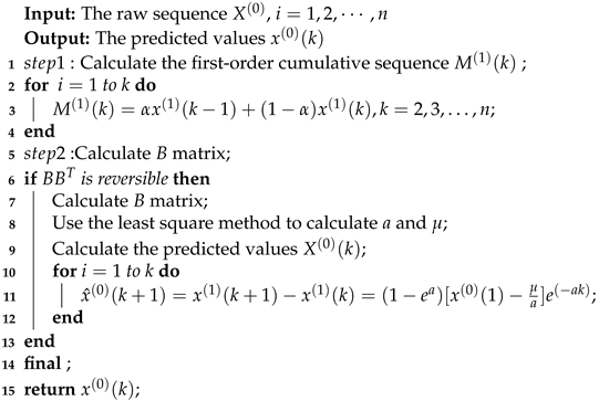 |
2.2. Grey Model of Caputo Type Fractional Derivative
| Algorithm 2: GM(,1) model. |
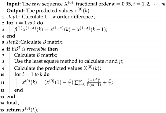 |
2.3. Accuracy Testing of GM(1,1) and GM(0.95,1)
3. Main Results
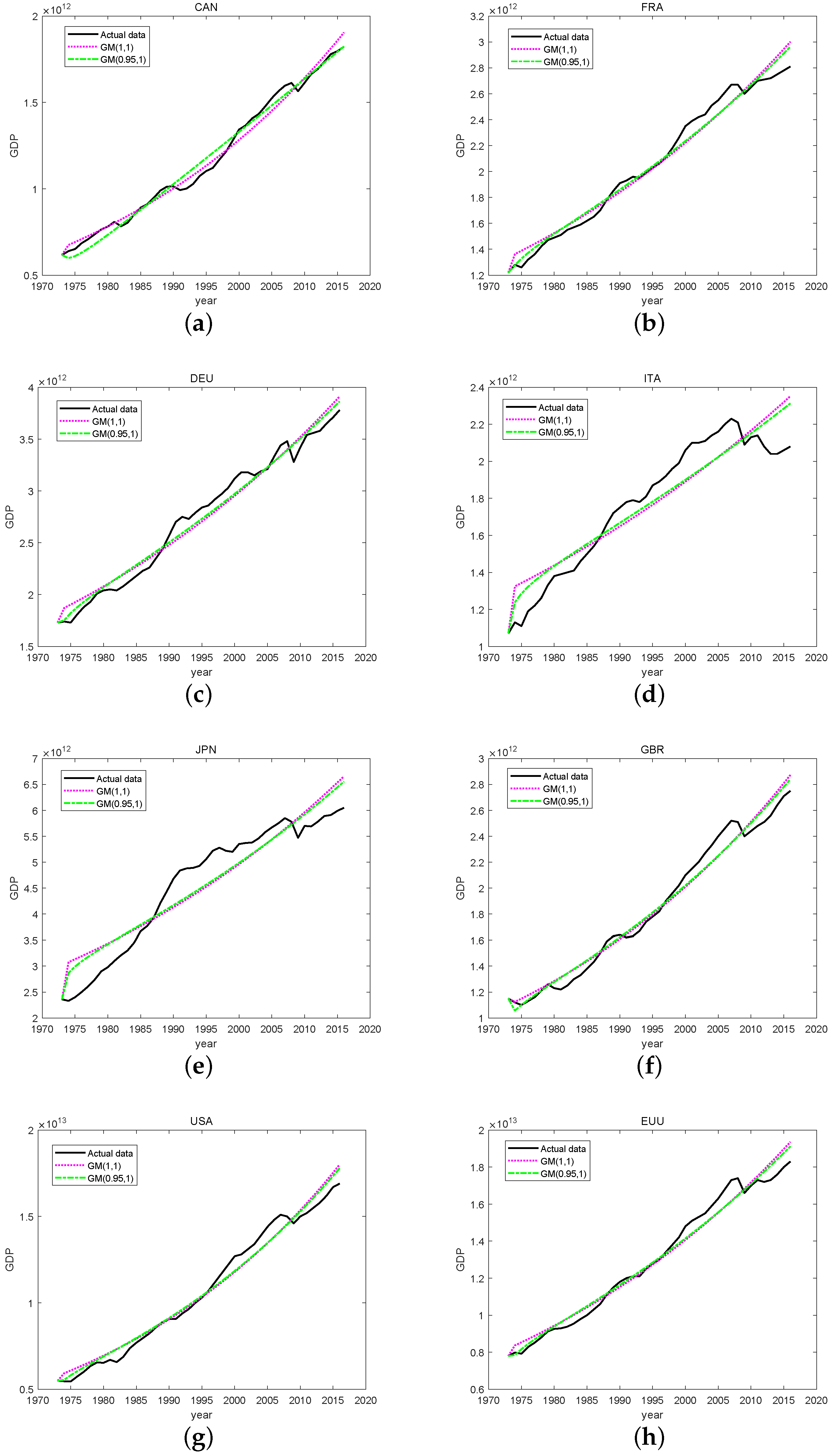
3.1. Fitting Result
3.2. Predicted Results
4. Conclusions
Author Contributions
Funding
Institutional Review Board Statement
Informed Consent Statement
Data Availability Statement
Acknowledgments
Conflicts of Interest
References
- Deng, J. Control problems of grey systems. Syst. Control. Lett. 1982, 1, 288–294. [Google Scholar]
- Deng, J. Essential Topics on Grey Systems: Theory and Applications; China Ocean Press: Beijing, China, 1988. [Google Scholar]
- Tien, T. A research on the grey prediction model GM(1,n). Appl. Math. Comput. 2012, 218, 4903–4916. [Google Scholar] [CrossRef]
- Li, D.; Chang, C.; Chen, C.; Kilicman, A. Forecasting short-term electricity consumption using the adaptive grey-based approach-An Asian case. Omega 2012, 40, 767–773. [Google Scholar] [CrossRef]
- Zhu, Z.; Cao, H. A fractional calculus based model for the simulation of an outbreak of dengue fever. J. Trop. Meteorol. 1998, 4, 359–365. [Google Scholar]
- Tien, T. The indirect measurement of tensile strength of material by the grey prediction model GMC(1, n). Meas. Sci. Technol. 2005, 16, 1322–1328. [Google Scholar] [CrossRef]
- Chen, C.; Tien, T. A new forecasting method for time continuous model of dynamic system. Appl. Math. Comput. 1996, 80, 225–244. [Google Scholar] [CrossRef]
- Chen, C.; Tien, T. A new transfer function model: The grey dynamic model GDM(2,2,1). Int. J. Syst. Sci. 1996, 27, 1371–1379. [Google Scholar] [CrossRef]
- Chen, C.; Tien, T. The indirect measurement of tensile strength by the deterministic grey dynamic model DGDM(1,1,1). Int. J. Syst. Sci. 1997, 28, 683–690. [Google Scholar] [CrossRef]
- Chen, C.; Tien, T. A new forecasting method of discrete dynamic system. Appl. Math. Comput. 1997, 86, 61–84. [Google Scholar] [CrossRef]
- Tien, T. A research on the prediction of machining accuracy by the deterministic grey dynamic model DGDM (1,1,1). Appl. Math. Comput. 2005, 161, 923–945. [Google Scholar] [CrossRef]
- Tien, T. The deterministic grey dynamic model with convolution integral DGDMC(1,n). Appl. Math. Model. 2009, 33, 3498–3510. [Google Scholar] [CrossRef] [Green Version]
- Tien, T. The indirect measurement of tensile strength for a higher temperature by the new model IGDMC(1,n). Measurement 2008, 41, 662–675. [Google Scholar] [CrossRef]
- Tien, T.; Chen, C. Forecasting CO2 output from gas furnace by a new transfer function model GDM(2,2,1). Syst. Anal. Model. Simul. 1998, 30, 265–287. [Google Scholar]
- Wu, L.; Liu, S.; Yao, L.; Yan, S.; Liu, D. Grey system model with the fractional order accumulation. Commun. Nonlinear Sci. Numer. Simul. 2013, 18, 1775–1785. [Google Scholar] [CrossRef]
- Awe, O.O.; Mudida, R.; Gil-Alana, L.A. Comparative analysis of economic growth in Nigeria and Kenya: A fractional integration approach. Int. J. Financ. Econ. 2021, 26, 1197–1205. [Google Scholar] [CrossRef]

| Accuracy Class | Index Critical Value | |
|---|---|---|
| P | C | |
| First-level | ||
| Second-level | ||
| Third-level | ||
| Forth-level | ||
| GM(1,1) | GM(0.95,1) | |||||
|---|---|---|---|---|---|---|
| MAD | BIC | MAD | BIC | |||
| CAN | 34414448765 | 0.9879086 | 48.94679 | 33734534311 | 0.9895514 | 48.80076 |
| FRA | 68364065162 | 0.9728951 | 50.37659 | 57357310718 | 0.9803684 | 50.05402 |
| DEU | 99453931115 | 0.9693005 | 50.94267 | 81811419026 | 0.9785968 | 50.58196 |
| ITA | 117484780283 | 0.8545935 | 51.33698 | 103872866630 | 0.8876252 | 51.07928 |
| JPN | 393677491323 | 0.8690739 | 53.69981 | 358667602223 | 0.8947864 | 53.48117 |
| GBR | 68468956596 | 0.9761038 | 50.34167 | 63648656598 | 0.9790246 | 50.2113 |
| USA | 467398760671 | 0.9766464 | 54.18997 | 420061610319 | 0.9809567 | 53.98594 |
| EUU | 441146078640 | 0.974133 | 54.12246 | 375276253076 | 0.9795674 | 53.88662 |
| GM(1,1) | GM(0.95,1) | |||
|---|---|---|---|---|
| P | C | P | C | |
| CAN | 1 | 0.1158 | 1 | 0.1097 |
| FRA | 1 | 0.1644 | 1 | 0.1401 |
| DEU | 1 | 0.1750 | 1 | 0.1462 |
| ITA | 0.9318 | 0.3811 | 1 | 0.3352 |
| JPN | 1 | 0.3601 | 1 | 0.3240 |
| GBR | 1 | 0.1543 | 1 | 0.1448 |
| USA | 1 | 0.1516 | 1 | 0.1374 |
| EUU | 1 | 0.1605 | 1 | 0.1429 |
| Year | Real Value | GM(1,1) | GM(0.95,1) | |||
|---|---|---|---|---|---|---|
| 2012 | 1693194096275.46 | 1725185175714.73 | 0.018896388 | 1698914426493.6 | 0.013003404 | |
| 2013 | 1735100681636.87 | 1768329586608.14 | 0.019151396 | 1730008754583.54 | 0.01207392 | |
| CAN | 2014 | 1779611206826.42 | 1812552977438.03 | 0.018511347 | 1761154346219.05 | 0.010233611 |
| 2015 | 1796369375909.66 | 1857882331947.61 | 0.034242574 | 1792351828024.82 | 0.024592371 | |
| 2016 | 1822735534879.33 | 1904345308704.84 | 0.04477068 | 1823601834354.28 | 0.033744816 | |
| 2012 | 2706807051174.77 | 2783679136379.47 | 0.027187873 | 2763087648243.83 | 0.019589538 | |
| 2013 | 2722404797996.28 | 2836504877221.62 | 0.042832675 | 2811708863760.12 | 0.033716494 | |
| FRA | 2014 | 2748201937555.55 | 2890333089526.44 | 0.051030214 | 2861110591403.97 | 0.040403851 |
| 2015 | 2777537939261.97 | 2945182797145.19 | 0.059418272 | 2911308024499.58 | 0.047233102 | |
| 2016 | 2810525379194.34 | 3001073384943.69 | 0.067997646 | 2962316477892.66 | 0.054205152 | |
| 2012 | 3559587403262.56 | 3646203072205.31 | 0.024214346 | 3620958453453.06 | 0.017123161 | |
| 2013 | 3577014590829.77 | 3710799857365.53 | 0.036536273 | 3680165471151.48 | 0.027979182 | |
| DEU | 2014 | 3646039898346.43 | 3776541050714.31 | 0.034668781 | 3740240804303.89 | 0.024723508 |
| 2015 | 3709597862509.39 | 3843446926791.69 | 0.035969522 | 3801200755783.78 | 0.024582414 | |
| 2016 | 3781698549834.74 | 3911538119324.91 | 0.034798444 | 3863061697944.44 | 0.021973994 | |
| 2012 | 2077060704620.29 | 2226728267130.19 | 0.070542436 | 2203799127286.2 | 0.059518811 | |
| 2013 | 2041165755679.07 | 2257377439911.16 | 0.106557569 | 2230621869130.45 | 0.093442093 | |
| ITA | 2014 | 2043486014884.01 | 2288448474580.78 | 0.121788468 | 2257706880792.64 | 0.106719059 |
| 2015 | 2063873410309.19 | 2319947177737.88 | 0.12618795 | 2285059098433.64 | 0.10925199 | |
| 2016 | 2083322583449.54 | 2351879435904.69 | 0.130711267 | 2312683379473.8 | 0.111867009 | |
| 2012 | 5778636370123.56 | 6186003375607.0 | 0.070242799 | 6126496812980.12 | 0.059947545 | |
| 2013 | 5894237388118.86 | 6300780322154.25 | 0.06974199 | 6231076789596.91 | 0.057907774 | |
| JPN | 2014 | 5914022267462.79 | 6417686874306.06 | 0.085903024 | 6337272922468.91 | 0.072296603 |
| 2015 | 5986140110537.86 | 6536762545398.38 | 0.091279223 | 6445116233574.44 | 0.075979338 | |
| 2016 | 6047894004051.61 | 6658047581909.06 | 0.100503733 | 6554637940727.12 | 0.08341123 | |
| 2012 | 2513321589693.39 | 2627121154069.95 | 0.046661814 | 2610421183989.1 | 0.04000844 | |
| 2013 | 2564904713179.98 | 2686476667723.88 | 0.049404948 | 2666139239003.77 | 0.04146064 | |
| GBR | 2014 | 2643243341332.76 | 2747173222309.94 | 0.040595918 | 2722980002145.48 | 0.031431819 |
| 2015 | 2705252231411.39 | 2809241116458.62 | 0.036620338 | 2780968390027.45 | 0.026187598 | |
| 2016 | 2753793133582.5 | 2872711333348.69 | 0.044622303 | 2840129727689.47 | 0.032774446 | |
| 2012 | 15542161722300 | 16194007236103.12 | 0.04477466 | 16081562735296.5 | 0.037520176 | |
| 2013 | 15802855301300 | 16628304384219.62 | 0.052424328 | 16493206997255.5 | 0.043873861 | |
| USA | 2014 | 16208861247400 | 17074248681192.62 | 0.053965968 | 16915003030371.25 | 0.04413599 |
| 2015 | 16672691917800 | 17532152484764.25 | 0.04982949 | 17347214175968.12 | 0.03875534 | |
| 2016 | 16920327941800 | 18002336529606.62 | 0.065227014 | 17790109806427.38 | 0.052669219 | |
| 2012 | 17206500000000 | 17871609712710.75 | 0.039047076 | 17744873110260.31 | 0.031678669 | |
| 2013 | 17251100000000 | 18232171082420.25 | 0.053882722 | 18079082959715.0 | 0.045033697 | |
| EUU | 2014 | 17551100000000 | 18600006810926.25 | 0.056818569 | 18419114699868.69 | 0.046540608 |
| 2015 | 17957000000000 | 18975263659086.88 | 0.054181314 | 18765086361202.56 | 0.042504798 | |
| 2016 | 18305200000000 | 19358091348673.75 | 0.057819199 | 19117117295279.62 | 0.044651218 |
Publisher’s Note: MDPI stays neutral with regard to jurisdictional claims in published maps and institutional affiliations. |
© 2022 by the authors. Licensee MDPI, Basel, Switzerland. This article is an open access article distributed under the terms and conditions of the Creative Commons Attribution (CC BY) license (https://creativecommons.org/licenses/by/4.0/).
Share and Cite
Liao, Y.; Wang, X.; Wang, J. Application of Fractional Grey Forecasting Model in Economic Growth of the Group of Seven. Axioms 2022, 11, 155. https://doi.org/10.3390/axioms11040155
Liao Y, Wang X, Wang J. Application of Fractional Grey Forecasting Model in Economic Growth of the Group of Seven. Axioms. 2022; 11(4):155. https://doi.org/10.3390/axioms11040155
Chicago/Turabian StyleLiao, Yumei, Xu Wang, and Jinrong Wang. 2022. "Application of Fractional Grey Forecasting Model in Economic Growth of the Group of Seven" Axioms 11, no. 4: 155. https://doi.org/10.3390/axioms11040155
APA StyleLiao, Y., Wang, X., & Wang, J. (2022). Application of Fractional Grey Forecasting Model in Economic Growth of the Group of Seven. Axioms, 11(4), 155. https://doi.org/10.3390/axioms11040155