A Comparative Study of Models for Heat Transfer in Bidisperse Gas–Solid Systems via CFD–DEM Simulations

Abstract

In this study, flow and heat transfers in bidisperse gas–solid systems were numerically investigated using the computational fluid dynamics–discrete element method (CFD–DEM). Three different models to close the gas–solid heat transfer coefficient for each species of bidisperse systems were compared in the simulations. The effect of the particle diameter ratio and particle number ratio between large and small particles on the particle mean temperature and temperature distribution of each species were systematically investigated. The simulation results show that differences in the particle mean temperature and temperature distribution profiles exist among the three heat transfer models at a higher particle number ratio. The differences between the effects of three heat transfer models on heat transfer properties in bidisperse systems with particle diameter ratios of up to 4 are marginal when the particle number ratio between small and large particles is 1.

1. Introduction

Fluidized bed reactors (FBRs), which have favorable heat and mass transfer characteristics, are frequently encountered in various industrial processes, such as fluid catalytic cracking, methanol to olefins, and circulating fluidized bed boilers. These processes usually involve highly endothermic or exothermic reactions, which have rapid heat removal or supply characteristics. It may easily generate hot or cold spots in FBRs, which seriously affect the performance of the reactors. Thus, the investigation of flow and heat transfers processes in gas–solid FBRs is of paramount importance.

In the past few decades, the fast growth in supercomputing power has made computational fluid dynamics (CFD) a promising tool to investigate flow, heat, and mass transfer in gas–solid FBD [1], with developed methods such as particle-resolved–direct numerical simulation (PR–DNS), computational fluid dynamics–discrete element method (CFD–DEM) and two-fluid model (TFM). The conservation governing equations in CFD–DEM or TFM are supplemented by the interphase drag, heat, and mass transfer correlations, which are needed for the closure of mass, momentum, and energy exchange term. Much effort has been invested to develop the constitutive models of the interphase drag [2,3,4,5,6] and heat/mass transfer correlations [7,8,9,10,11,12,13,14] using PR–DNSs and experimental methods. It should be noted that these models mainly focus on monodisperse gas–solid systems. However, the polydispersity of particle size is common and plays an important role in determining the performance of practical FBRs.

Currently, several interphase drag models for the closure of the momentum exchange term in bidisperse gas–solid FBRs have been proposed in relevant studies in the literature [15,16,17,18,19,20,21]. These studies adopted the same strategy, which is a correction to the monodisperse drag models to predict the drag force on each species of bidisperse systems. However, the correlations to describe the heat/mass transfer behavior of bidisperse systems are relatively rare. Tavassoli et al. [22] investigated the heat transfer behavior of bidisperse systems with a particle size of 2 using PR–DNSs. They found that the model coupled with the Sauter mean diameter, and the monodisperse heat transfer correlations may accurately predict the overall heat transfer coefficient. Lu et al. [23] explored the mass transfer behavior of bidisperse systems with a particle size ratio of 1.5. They formulated a refitted Gunn correlation in which the Reynolds number and Nusselt number are obtained based on the particle diameter of each species. They also found that the overall mass transfer coefficient can be accurately predicted via the monodisperse correlation and an appropriate equivalent diameter. Huang et al. [24] investigated flow and heat transfers in bidisperse systems with particle diameter ratios ranging from 1:2 to 1:4 using PR–DNSs. They built models for the overall correlation and the heat transfer correlation of each species via a correction to the monodisperse correaltion. They found the correction term is only closed as a function of the total solid volume fraction and scaled particle diameter.

As discussed in the aforementioned studies, it is evident that there are three models available to close the heat transfer coefficient of each species in bidisperse gas–solid systems. Firstly, the heat transfer coefficient of each species is calculated via the monodisperse correlation, and the characteristic diameters of each species in Reynolds and Nusselt numbers are defined as the Sauter mean diameter. Secondly, the particle diameter of each species is used to calculate their respective Reynolds and Nusselt numbers in the monodisperse correlation. Finally, the heat transfer correlation for each species is obtained via a correction to the monodisperse heat transfer correlation. These models mentioned above have not yet been used to close the interphase heat transfer coefficient in CFD–DEM and TFM simulations for bidisperse gas–solid FBRs. Therefore, this study attempts to take a step toward understanding the effect of the heat transfer models for bidisperse systems on the interphase heat transfer process. Flow and heat transfers in bidisperse gas–solid FBRs were simulated via CFD–DEM. Three different interphase heat transfer constitutive correlations were taken into account in this study. The numerical methods for flow and heat transfers in gas–solid FBRs are described in Section 2. Validation for the adopted numerical method is performed in Section 3.1. The effect of the particle diameter ratio and particle number ratio between large and small particles on the simulation results are reported and discussed in Section 3.2 and Section 3.3. The main findings are summarized in Section 4.

2. Numerical Method

CFD–DEM was used to solve the conservation equations describing the flow and heat transfer process in gas–solid FBR. It is based on continuum fixed-grid (Eulerian) modeling of the gas phase and discrete (Lagrangian) modeling of the particle phase. The simulations were performed using Multiphase Flow with Interphase eXchanges (MFIX) version 19.3.1. More details on the theory and numerical method of MFIX can be found at https://mfix.netl.doe.gov/, accessed on 27 February 2022 [25,26,27]. The conservation governing equations of the gas and solid phase, and the implementation process, can be found in a study by Garg et al. [28].

2.1. Gas-Phase Modeling

The conservation equations for gas-phase mass and momentum are written as follows:

$$\frac{\partial }{\partial t}\left({\epsilon }_f{\rho }_f\right)+\nabla \cdot \left({\epsilon }_f{\rho }_f\mathit{u}\right)=0$$

(1)

$$\frac{\partial }{\partial t}\left({\epsilon }_f{\rho }_f\mathit{u}\right)+\nabla \cdot \left({\epsilon }_f{\rho }_f\mathit{u}\mathit{u}\right)=-{\epsilon }_f\nabla p-\nabla \cdot \left({\epsilon }_f{\mathit{\tau }}_f\right)+{\mathit{S}}_p+{\epsilon }_f{\rho }_f\mathit{g}$$

(2)

where ${\epsilon }_f$, ${\rho }_f$, and $\mathit{u}$ denote the volume fraction, density, and velocity of the gas phase, respectively. $g$ denotes the gravitational acceleration. $p$, ${\mathit{\tau }}_f$, and ${\mathit{S}}_p$ represent the pressure, stress tensor, and momentum source term of the gas phase, respectively.

$${\mathit{S}}_p={\displaystyle \sum _{}\frac{{\beta }_p{V}_p}{1-{\epsilon }_f}}\left({\mathit{v}}_p-\mathit{u}\right)$$

(3)

where $V_p$ and ${\mathit{v}}_p$ denote the volume and velocity of particle. ${\beta }_p$ is the interphase drag coefficient on the individual particle, which was closed in this study using the BVK model [15].

$$\begin{array}{l}{\beta }_p=y_p\left(\begin{array}{l}\frac{10\left(1-{\epsilon }_f\right)}{{\epsilon }_f^2}+{\epsilon }_f^2\left(1+1.5{\left(1-{\epsilon }_f\right)}^{0.5}\right)\\ +\frac{0.413R{e}_{32}}{24{\epsilon }_f^2}\left[\frac{{\epsilon }_f^{-1}+3{\epsilon }_f\left(1-{\epsilon }_f\right)+8.4R{e}_{32}^{-0.343}}{1+{10}^{3\left(1-{\epsilon }_f\right)}R{e}_{32}^{-\frac{1+4\left(1-{\epsilon }_f\right)}{2}}}\right]\end{array}\right)\\ \end{array}$$

(4)

where $y_p=d_p/d_{32}$ is the scaled particle diameter; $d_{32}$ is the Sauter mean diameter. $R{e}_{32}$ is defined as

$$R{e}_{32}=\frac{d_{32}{\epsilon }_f{\rho }_f\left|{\mathit{v}}_p-\mathit{u}\right|}{{\mu }_f}$$

(5)

where ${\mu }_f$ is the viscosity of the gas phase.

The energy equation for the gas phase is written as

$$\frac{\partial \left({\rho }_f{C}_{Pf}{\epsilon }_f{T}_f\right)}{\partial t}+\nabla \cdot \left({\rho }_f{C}_{Pf}{\epsilon }_f{T}_f\mathit{u}\right)=\nabla \cdot \left(k_f^{*}{\epsilon }_f\nabla T_f\right)+Q_f$$

(6)

where $T_f$, $C_{Pf}$, and $k_f^{*}$ are the temperature, specific heat capacity, and effective conductivity of the gas phase, respectively. $Q_f$ is the source term of the interphase heat transfer.

$$Q_f=\frac{{\displaystyle \sum _{}{h}_{fp}{A}_p\left(T_p-T_f\right)}}{V_{\mathrm{cell}}}$$

(7)

where $h_{fp}$ is the interphase heat transfer coefficient, $h_{fp}=\frac{k_f^{*}N{u}_p}{d_p}$, and $N{u}_p$ is the Nusselt number. $A_p$ and $T_p$ are the particle surface area and temperature, and V_cell is the grid volume.

$N{u}_p$ is closed using the models proposed by Gunn (1978) [14] and Huang et al. (2019) [9] in monodisperse systems. The models of Gunn (1978) [14] and Huang et al. (2019) [9] are given in Equations (8) and (9), respectively.

$$N{u}_p=\left(7-10{ϵ}_f+5{ϵ}_f{}^2\right)\left[1+0.7R{e}_p^{0.2}{\mathrm{Pr}}^{0.33}\right]+\left(1.33-2.40{ϵ}_f+1.20{ϵ}_{{}_f}^2\right)R{e}_p^{0.7}{\mathrm{Pr}}^{0.33}$$

(8)

$$N{u}_p=\left(7-10{ϵ}_f+5{ϵ}_f{}^2\right)\left[1+0.17R{e}_p^{0.2}{\mathrm{Pr}}^{0.33}\right]+\left(1.33-2.25{ϵ}_f+1.16{ϵ}_{{}_f}^2\right)R{e}_p^{0.7}{\mathrm{Pr}}^{0.33}$$

(9)

where $\mathrm{Pr}={\mu }_f{C}_{p,f}/k_f$, $k_f$ is the conductivity of the gas phase.

In this study, three different interphase heat transfer models were considered in bidisperse gas–solid systems: (1) $N{u}_p$ was closed using Equation (9), while $N{u}_p$ and $R{e}_p$ in Equation (9) were calculated using the particle diameter of each species; the model was denoted as Huang_pcf (2019); (2) $N{u}_p$ was also closed using Equation (9), while the Sauter mean diameter was used to calculate $N{u}_p$ and $R{e}_p$; the model was denoted as Huang (2019); (3) the heat transfer correlation for each species proposed by Huang et al. (2021) [24] were obtained with a correction to the monodisperse heat transfer correlation, as follows:

$$N{u}_p=Nu\left({ϵ}_s,R{e}_{31}\right)\left(0.5f\left({ϵ}_s\right)\left(y_p{}^2+y_p\right)+\left(1-f\left({ϵ}_s\right)\right)y_p^{\frac{0.3472R{e}_{31}}{R{e}_{31}+1}}\right)$$

(10)

$$f\left({ϵ}_s\right)={ϵ}_s\left(3.211{ϵ}_s{}^2-2.42{ϵ}_s+0.9398\right)$$

(11)

where $Nu\left({ϵ}_s,R{e}_{31}\right)$ is calculated with Equation (9), and $R{e}_{31}$ is obtained via an approximate equivalent diameter $d_{31}$; for details, the reader can refer to [24]. $y_p=d_p/d_{31}$, and the solid volume fraction is defined as ${ϵ}_s=1-{ϵ}_f$. It is worth mentioning that the particle–particle and particle–wall heat transfers were neglected in this study [29].

2.2. Discrete Particle Phase

The particle phase modeling is based on tracking each particle. The motion of a single particle is described by Newton’s equation as follows:

$$m_p\frac{d^2{\mathit{x}}_p}{d{t}^2}=-V_p\nabla p+\frac{{\beta }_p{V}_p}{1-{\epsilon }_f}\left({\mathit{v}}_p-\mathit{u}\right)+m_{p}g+F_{c,p}$$

(12)

$$I_p\frac{d{\omega }_p}{dt}=To{r}_p$$

(13)

where $m_p$ and ${\mathit{x}}_p$ are the particle mass and position. $F_{c,p}$ is the particle–particle or particle–wall collision forces calculated by the soft-sphere approach; the linear spring–dashpot model was used. The parameter settings for the contact model are summarized in

Table 1. Physical properties of the two phases.

Simulation Parameters	Value	Simulation Parameters	Value
Particle diameter, dp	1.0 × 10−3 m	Gas viscosity	1.8 × 10−5 Pa·s
Particle heat capacity	840 J/(kg·K)	Gas density	1.3 kg/m3
Particle density	2500 kg/m3	Gas heat capacity	1010 J/(kg·K)
Initial particle temperature	363.15 K	Gas conductivity	0.02552 W/(m·K)
Particle conductivity	1.4 W/(m·K)	Normal spring constant	500 N/m
Particle–particle and particle–wall friction coefficient	0.3	Restitution coefficient for inter-particle collisions and particle–wall collisions	0.97
Ratio of the tangential spring constant to normal spring constant for inter-particle collisions and particle–wall collisions	0.286	Ratio of the tangential damping factor to the normal damping factor for inter-particle collisions and particle–wall collisions	0.5

. $I_p$, ${\omega }_p$, and $To{r}_p$ are the moment of inertia, the angular velocity, and torque of the particle.

The energy equation of each particle is written as

$${\rho }_p{V}_p{C}_{p,p}\frac{d{T}_p}{dt}=h_{fp}{A}_p\left(T_f-T_p\right)$$

(14)

where ${\rho }_p$ and $C_{p,p}$ denote the density and specific capacity of the particle phase, respectively.

3. Results and Discussion

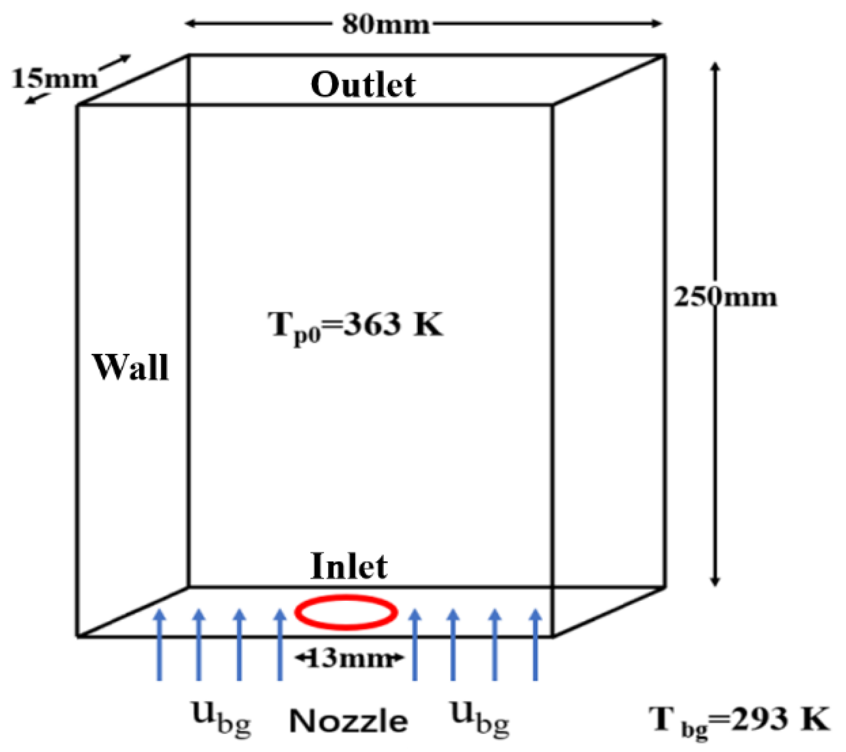
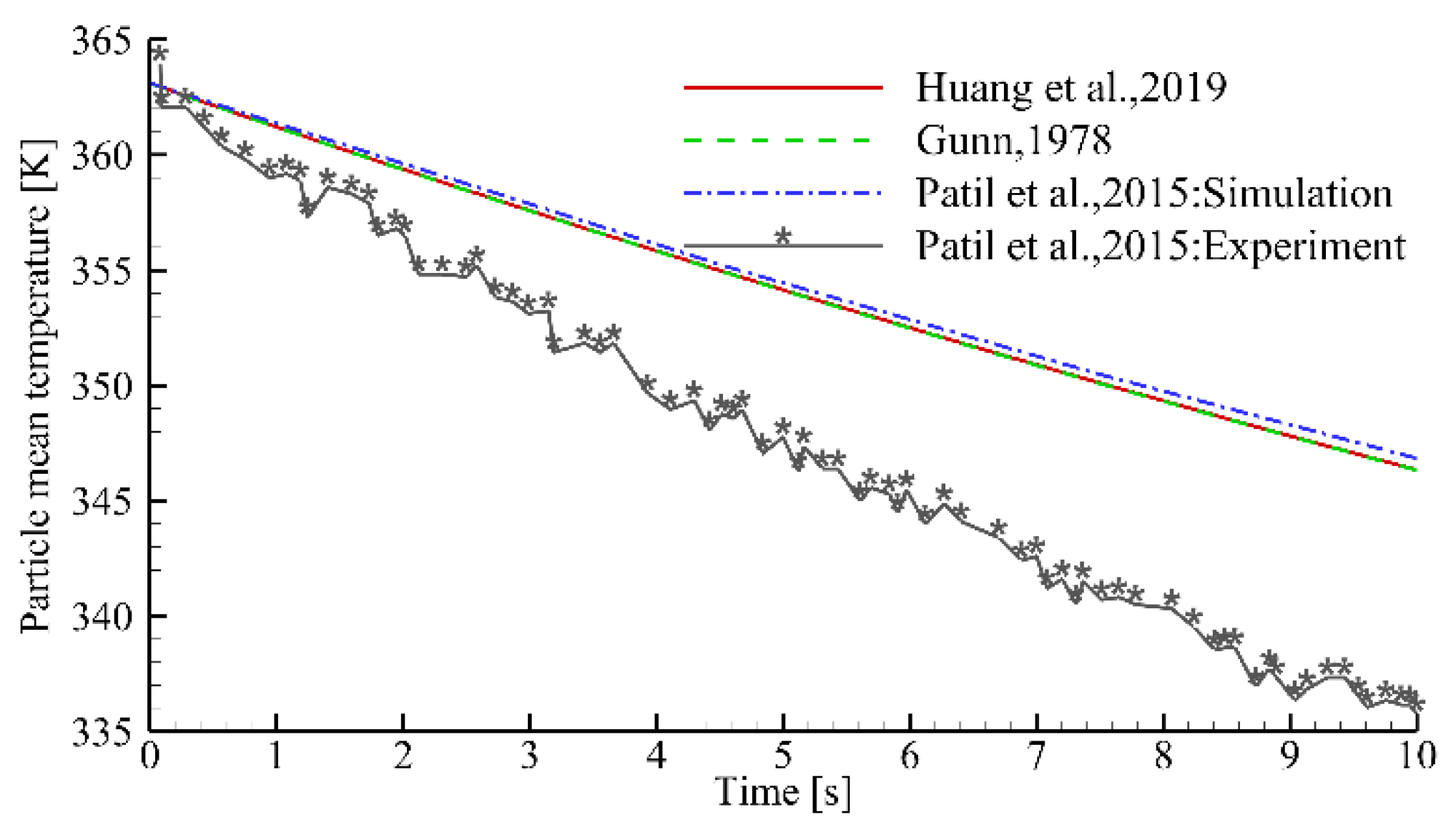
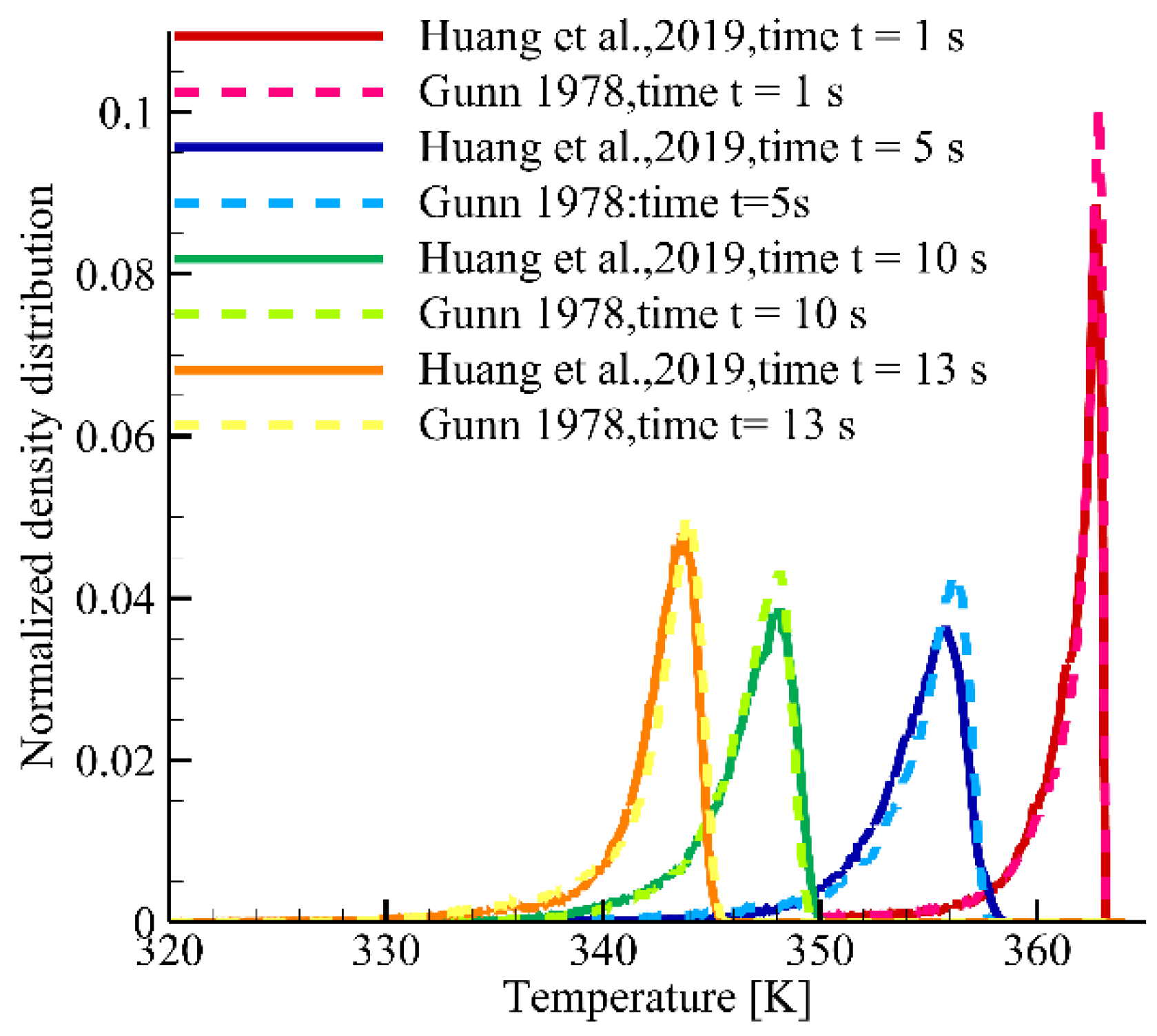
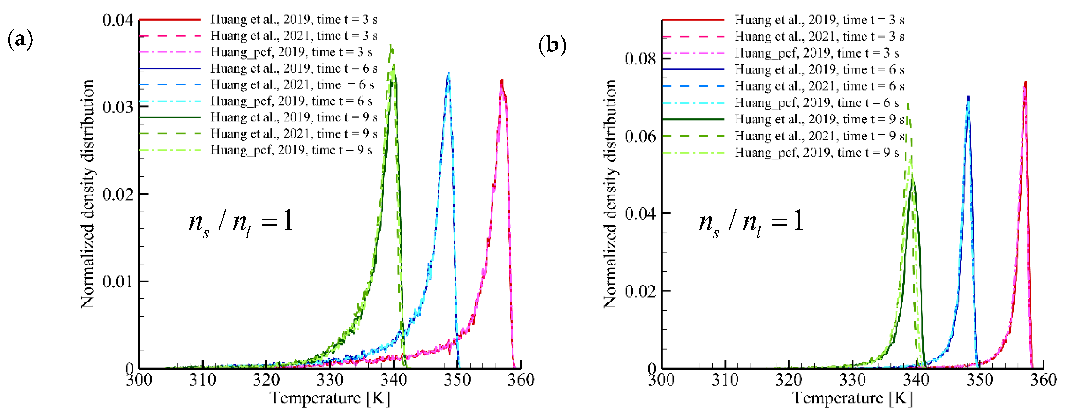
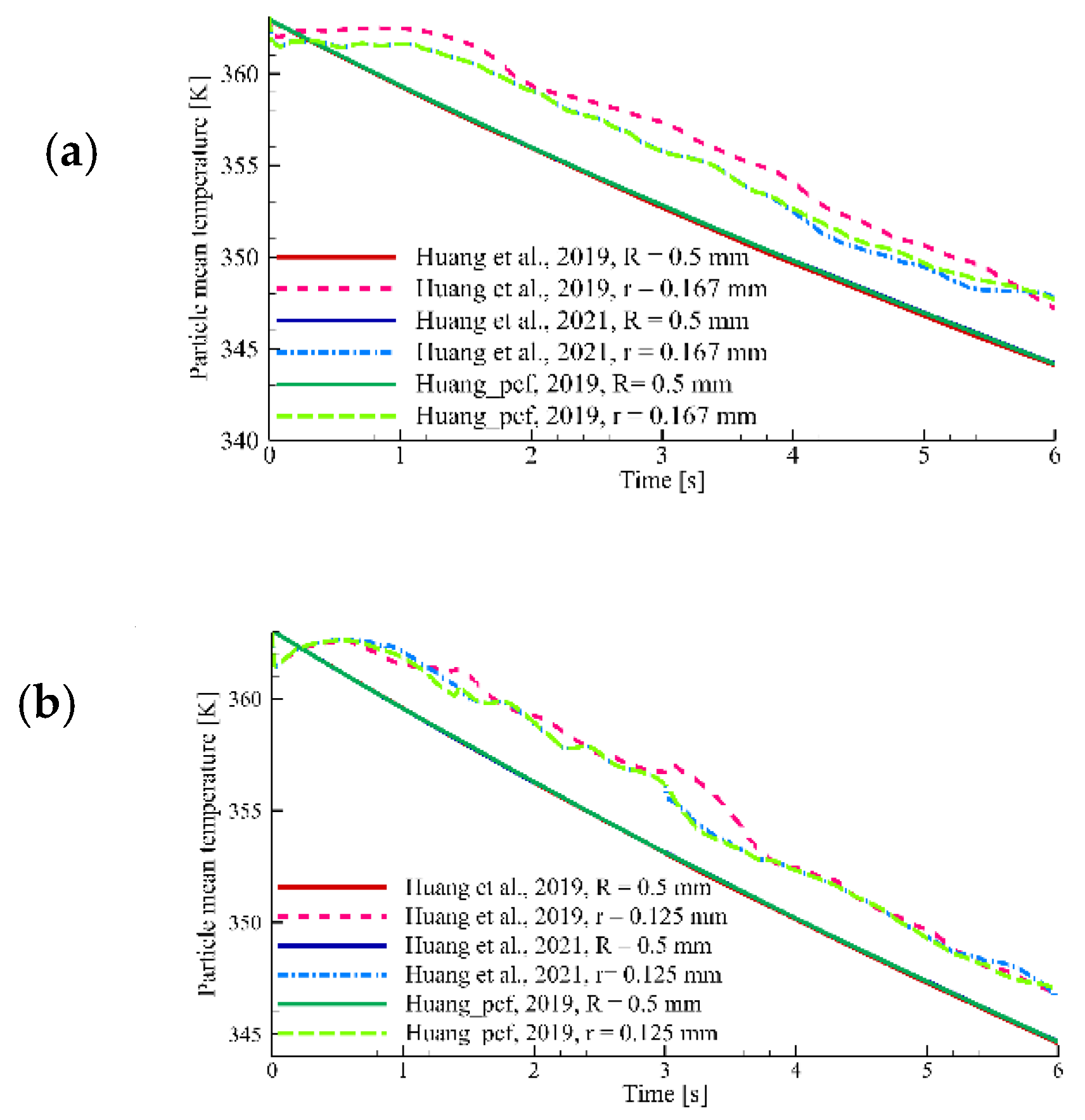
3.1. Validation

To validate the adopted thermal CFD–DEM, several simulations were carried out regarding flow and heat transfers in pseudo-2D FBRs based on experimental investigations [30]. The simulation setup is shown in Figure 1. In the experiment, a cold background gas (T_bg = 293.15 K) entered from the inlet, except for the nozzle of size 13 mm. The inlet velocity was 1.2 m/s, and the pressure outlet boundary condition was used. No-slip and adiabatic boundary conditions were imposed on the wall. The wall heat loss was neglected. The physical properties of the two phases are shown in Table 1. Four different Eulerian grid numbers (79659, 23100, 19200, and 10600) were considered to investigate the influence of the grid size on the simulation results; the averaged grid sizes (in terms of the edge length of a cubic grid) are approximately equal to 1.5 d_p, 2.2 d_p, 2.5 d_p, and 3 d_p, respectively. The particles’ mean temperature vs. time from 0 s to 5 s is shown in Figure 2. It can be found that the effect of the grid size on the particle mean temperature is marginal. The grid numbers 23100, 19200, and 10600 lead to similar simulation results. Therefore, the grid number of 19200 was adopted for all simulations in this study. Figure 3 shows the variations in the local solid volume fraction and particle Reynolds number with the flow time in the cube region centered on the point of 40 mm × 20 mm × 7.5 mm. The cubic region size was 6.6 d_p × 6.6 d_p × 7.5 d_p. It can be found that the local solid volume fraction and particle Reynolds number fluctuate around different constant values. This demonstrates that the gas–solid flow behavior reaches the statistical steady state rapidly. Figure 4 shows the comparison of the particles’ mean temperature obtained from experiments with the prediction from simulations. The closure models proposed by Gunn (1978) [14] and Huang et al. (2019) [9] for the interphase heat transfer coefficient were used. It can be found that the results obtained from the present study agree well with those from the simulations performed by Pati et al. In addition, the simulation results are in reasonable agreement with experiment data. The discrepancy between the simulation results and the experimental data might attribute to the fact that the wall heat loss in the simulation was neglected. It can be concluded from the simulation results that the current numerical method is reliable for solving flow and heat transfer problems in gas–solid systems. Figure 5 shows that the temperature distributions from the simulations by adopting the models of Gunn (1978) [9] and Huang et al. (2019) [14] are almost the same. It means that the effect of the interphase heat transfer models on the heat transfer process can be ignored in present systems.

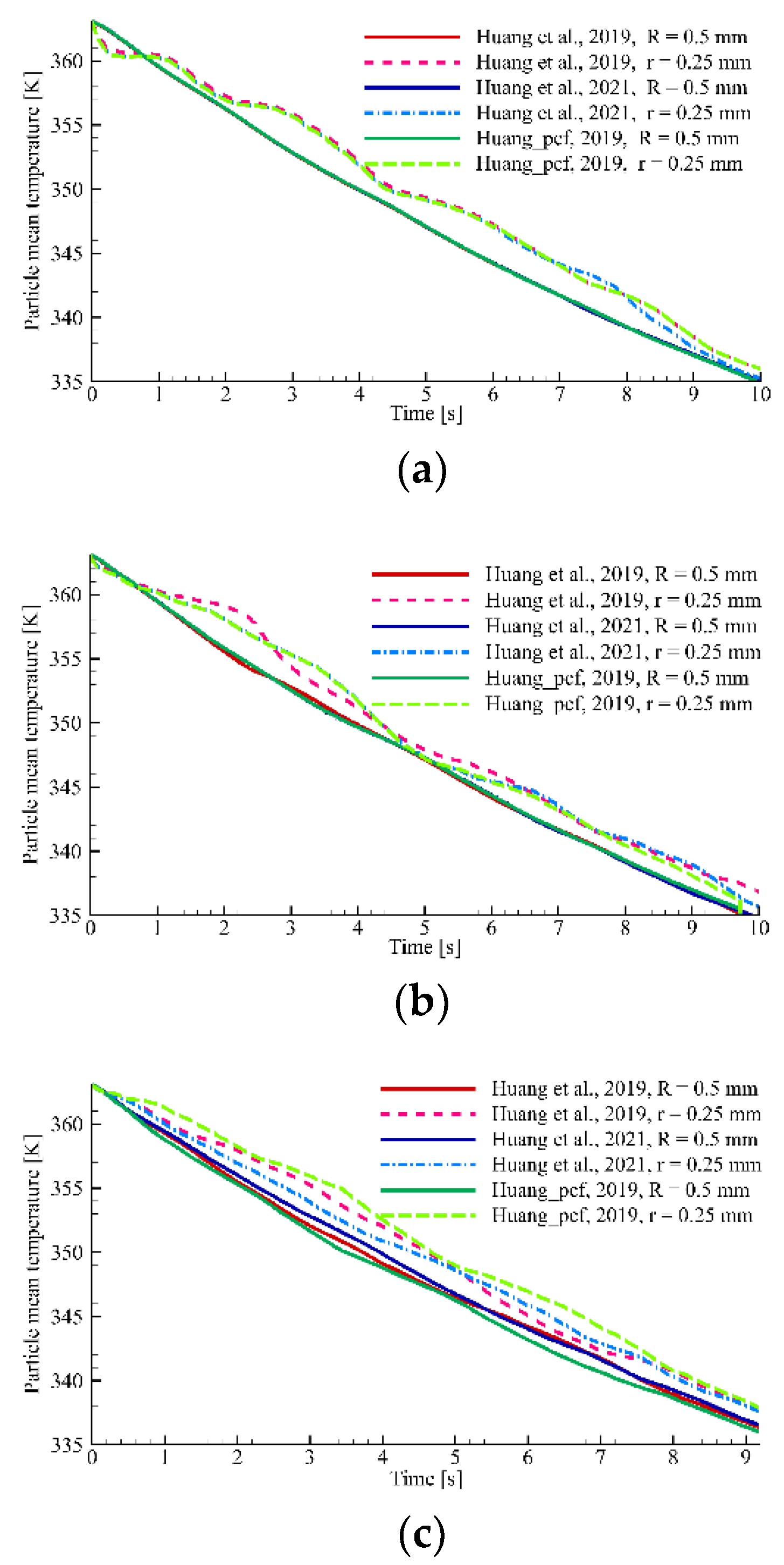
3.2. Effect of the Particle Number Ratio

Simulations using different interphase heat transfer models for the gas–solid bidisperse systems with three different particle number ratios were performed. The reactor and the physical properties of the two phases were the same as those mentioned in the previous section. The particle diameters for large and small particles were 1 mm and 0.5 mm, respectively. The particle number ratios between small and large particles ($n_s/n_l$) were 1, 2, and 4. The same bed masses (40.8 g) were used for the three particle number ratios. Figure 6 and Figure 7 show the particles’ mean temperature and particle temperature distributions of large and small particles, respectively. It can be found from Figure 6 that the mean temperatures of large particles for different particle number ratios are lower than those of small particles. This can be attributed to the fact that larger values in $y_p$ and $R{e}_p$ for large particles result in greater values in $N{u}_p$. It can be found that the simulation results of the particle mean temperatures and paricle temperature distributions of large and small particles using three interphase heat transfer models are the same at $n_s/n_l=1$, while minor differences are found at $n_s/n_l=2$ and $4$. This is due to the fact that a higher value in $n_s/n_l$ will result in a greater difference between the equivalent diameter and the diameter of each species used to calculate the Reynolds number in three heat transfer models. As shown in Figure 6c, the minimum and maximum temperature difference between large and small particles were obtained from the simulations using Huang et al. (2021) [24] and Huang et al. (2019) [9], respectively; for example, the respective values were 1 K and 5 K at 3.5 s for $n_s/n_l=4$. Furthermore, Figure 7c,e show that the differences between the effect of the interphase heat transfer models on the temperature distribution profile of large particles are marginal. However, the interphase models have greater effects on the temperature distribution profile of small particles, as shown in Figure 7d,f. These results demonstrate that the interphase heat transfer model plays an important role in the simulations for the gas–solid bidisperse system at a higher particle number ratio.

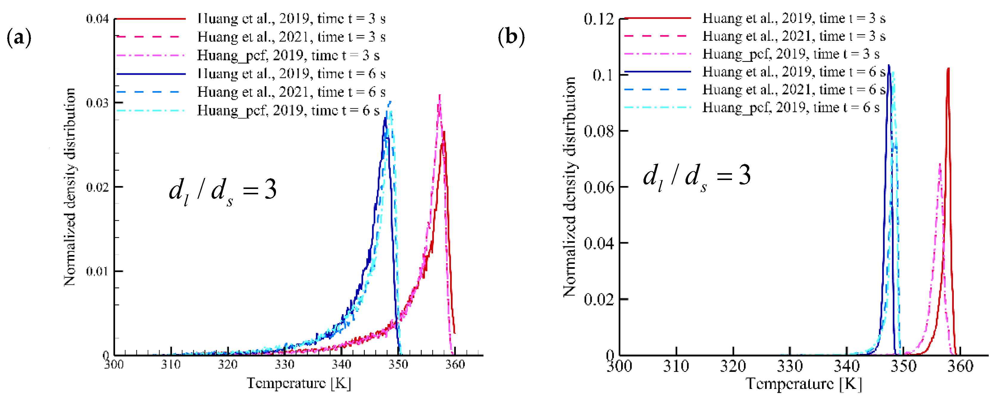
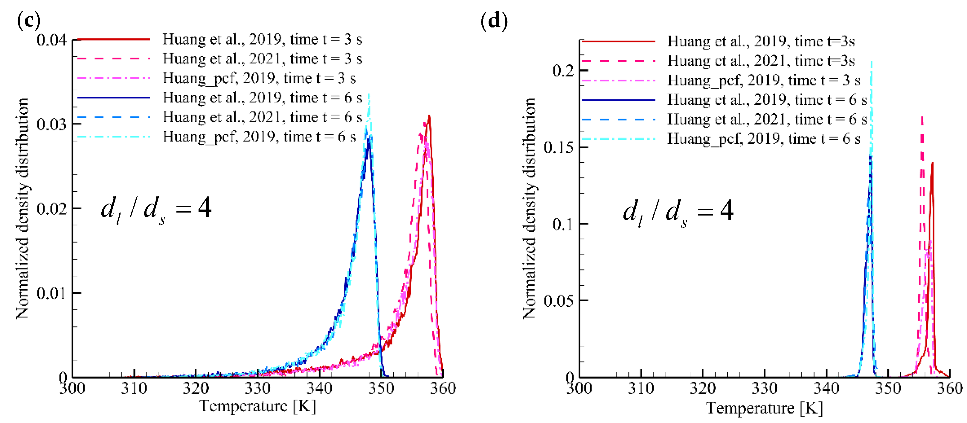
3.3. Effect of the Particle Diameter Ratio

The effect of the interphase heat transfer models on the particles’ mean temperatures and temperature distributions of large and small particles were investigated, and the results are presented in this section. Three particle diameter ratios between large and small particles ($d_l/d_s$ = 2, 3, and 4) were considered. Bed masses of 40.8 g and a particle number ratio ($n_s/n_l$) of 1 were used. Figure 8 shows the variation in particles’ mean temperature against the flow time at $d_l/d_s=$ 3 and 4. It can be found that the particle mean temperatures of large particles obtained from three interphase heat transfer models are the same at different particle diameter ratios, while the minor differences for the small particle mean temperature obtained from the model of Huang et al. (2019) can be found at $d_l/d_s=$ 3 and 4. For instance, the maximum temperature difference between Huang et al. (2021) and Huang et al. (2019) at $d_l/d_s=$ 3 and 4 can reach 1.5 K and 2 K, respectively. Figure 9 shows the temperature distribution profiles with different particle diameter ratios. Compared with the temperature distribution profile for the small particles predicted by the models of Huang et al. (2021) and Huang_pcf (2019), a higher value in the small particle temperature obtained from the model of Huang et al. (2019) can also be found. This indicates that the effect of the interphase heat transfer model on the heat transfer properties is marginal in this study. This can be attributed to the fact that the same particle number ratio ($n_s/n_l$) of 1 was adopted for different particle diameter ratios. Therefore, the equivalent diameter was very close to the large particle diameter, especially for the greater value of $d_l/d_s$. However, an increase in $n_s/n_l$ drastically increases the computation resources. Therefore, greater values in $n_s/n_l$ for different values of $d_l/d_s$ were not considered in this study.

4. Conclusions

The flow and heat transfer in bidisperse gas–solid systems were numerically investigated via CFD–DEM. Three models to close the interphase heat transfer coefficient were taken into account. The effects of particle diameter and particle number ratio between large and small particles on the particle mean temperature and temperature distribution of each species were systematically investigated.

The simulation results show that the mean temperatures of large particles for three particle number ratios were lower than those of small particles. The particles’ mean temperatures and temperature distributions of each species for three interphase heat transfer models were the same at $n_s/n_l=1$. The difference in simulation results among three different models were found at $n_s/n_l=2$ and $4$. The values of 1 K and 5 K for the temperature difference between large and small particles were obtained from the simulations using Huang et al. (2021) and Huang et al. (2019) at $n_s/n_l=4$, respectively. The reason for the difference can be attributed to the fact that a greater difference between the equivalent diameter and the diameter of each species can be obtained at higher values of $n_s/n_l$.

The effects of the gas–solid heat transfer models on the heat transfer of bidisperse systems with the particle diameter ratios ranging from 2 to 4 were investigated when the particle number ratio between small and large particles is 1. It can be found that the particle mean temperatures of large particles obtained from three interphase heat transfer models were the same at different particle diameter ratios. This is due to the fact that the same particle numbers ratio ($n_s/n_l$) of 1, which results in the marginal difference between equivalent diameter and large particle diameter, was adopted for different particle diameter ratios. However, a higher value of $n_s/n_l$ requires more computation resources and, therefore, was not considered in this study. Thus, a greater value of $n_s/n_l$ for different $d_l/d_s$ will be considered in the future. Furthermore, marginal effects on small particles were found at $d_l/d_s=$3 and 4 when the interphase heat transfer model of Huang et al. (2019) was used. It was found that the maximum temperature difference between Huang et al. (2021) and Huang et al. (2019) at $d_l/d_s=$3 and 4 can reach 1.5 K and 2 K, respectively.

References

1. Baltussen, M.W.; Buist, K.A.; Peters, E.A.J.F.; Kuipers, J.A.M. Multiscale modelling of dense gas-particle flows. In Advances in Chemical Engineering; Academic Press: Cambridge, MA, USA, 2018; pp. 1–52. [Google Scholar]
2. Hill, R.J.; Koch, D.L.; Ladd, A.J.C. The first effects of fluid inertia on flows in ordered and random arrays of spheres. J. Fluid Mech. 2001, 448, 213–241. [Google Scholar] [CrossRef]
3. Hill, R.J.; Koch, D.L.; Ladd, A.J.C. Moderate-Reynolds-number flows in ordered and random arrays of spheres. J. Fluid Mech. 2001, 448, 243–278. [Google Scholar] [CrossRef]
4. Zhou, Q.; Fan, L.-S. Direct numerical simulation of low-Reynolds-number flow past arrays of rotating spheres. J. Fluid Mech. 2015, 765, 396–423. [Google Scholar] [CrossRef]
5. Tang, Y.; Peters, E.A.J.F.; Kuipers, J.A.M. Direct numerical simulations of dynamic gas-solid suspensions. AIChE J. 2016, 62, 1958–1969. [Google Scholar] [CrossRef] [Green Version]
6. Tenneti, S.; Garg, R.; Subramaniam, S. Drag law for monodisperse gas–solid systems using particle-resolved direct numerical simulation of flow past fixed assemblies of spheres. Int. J. Multiph. Flow 2011, 37, 1072–1092. [Google Scholar] [CrossRef]
7. Deen, N.G.; Kriebitzsch, S.H.; van der Hoef, M.A.; Kuipers, J.A.M. Direct numerical simulation of flow and heat transfer in dense fluid–particle systems. Chem. Eng. Sci. 2012, 81, 329–344. [Google Scholar] [CrossRef]
8. Feng, Z.-G.; Musong, S.G. Direct numerical simulation of heat and mass transfer of spheres in a fluidized bed. Powder Technol. 2014, 262, 62–70. [Google Scholar] [CrossRef]
9. Huang, Z.; Zhang, C.; Jiang, M.; Wang, H.; Zhou, Q. Effects of particle velocity fluctuations on inter-phase heat transfer in gas-solid flows. Chem. Eng. Sci. 2019, 206, 375–386. [Google Scholar] [CrossRef]
10. Municchi, F.; Radl, S. Momentum, heat and mass transfer simulations of bounded dense mono-dispersed gas-particle systems. Int. J. Heat Mass Transf. 2018, 120, 1146–1161. [Google Scholar] [CrossRef] [Green Version]
11. Sun, B.; Tenneti, S.; Subramaniam, S. Modeling average gas–solid heat transfer using particle-resolved direct numerical simulation. Int. J. Heat Mass Transf. 2015, 86, 898–913. [Google Scholar] [CrossRef] [Green Version]
12. Tavassoli, H.; Kriebitzsch, S.; van der Hoef, M.; Peters, E.; Kuipers, H. Direct numerical simulation of particulate flow with heat transfer. Int. J. Multiph. Flow 2013, 57, 29–37. [Google Scholar] [CrossRef]
13. Tenneti, S.; Sun, B.; Garg, R.; Subramaniam, S. Role of fluid heating in dense gas–solid flow as revealed by particle-resolved direct numerical simulation. Int. J. Heat Mass Transf. 2013, 58, 471–479. [Google Scholar] [CrossRef]
14. Gunn, D.J. Transfer of heat or mass to particles in fixed and fluidized beds. Int. J. Heat Mass Transf. 1978, 21, 467–476. [Google Scholar] [CrossRef]
15. Beetstra, R.; van der Hoef, M.A.; Kuipers, J.A.M. Drag force of intermediate Reynolds number flow past mono- and bidisperse arrays of spheres. AIChE J. 2007, 53, 489–501. [Google Scholar] [CrossRef]
16. Cello, F.; Di Renzo, A.; Di Maio, F.P. A semi-empirical model for the drag force and fluid–particle interaction in polydisperse suspensions. Chem. Eng. Sci. 2010, 65, 3128–3139. [Google Scholar] [CrossRef]
17. Holloway, W.; Yin, X.; Sundaresan, S. Fluid-particle drag in inertial polydisperse gas–solid suspensions. AIChE J. 2010, 56, 1995–2004. [Google Scholar] [CrossRef]
18. Rong, L.W.; Dong, K.J.; Yu, A.B. Lattice-Boltzmann simulation of fluid flow through packed beds of spheres: Effect of particle size distribution. Chem. Eng. Sci. 2014, 116, 508–523. [Google Scholar] [CrossRef]
19. Sarkar, S.; van der Hoef, M.A.; Kuipers, J.A.M. Fluid–particle interaction from lattice Boltzmann simulations for flow through polydisperse random arrays of spheres. Chem. Eng. Sci. 2009, 64, 2683–2691. [Google Scholar] [CrossRef]
20. Yin, X.; Sundaresan, S. Fluid-particle drag in low-Reynolds-number polydisperse gas-solid suspensions. AIChE J. 2009, 55, 1352–1368. [Google Scholar] [CrossRef]
21. Duan, F.; Zhao, L.; Chen, X.; Zhou, Q. Fluid-particle drag and particle-particle drag in low-Reynolds-number bidisperse gas-solid suspensions. Phys. Fluids 2020, 32, 113311. [Google Scholar] [CrossRef]
22. Tavassoli, H.; Peters, E.; Kuipers, J.A.M. Direct numerical simulation of non-isothermal flow through dense bidisperse random arrays of spheres. Powder Technol. 2017, 314, 291–298. [Google Scholar] [CrossRef] [Green Version]
23. Lu, J.; Peters, E.A.; Kuipers, J.A. Direct numerical simulation of mass transfer in bidisperse arrays of spheres. AIChE J. 2020, 66, e16786. [Google Scholar] [CrossRef] [Green Version]
24. Huang, Z.; Wang, L.; Li, Y.; Zhou, Q. Direct numerical simulation of flow and heat transfer in bidisperse gas-solid systems. Chem. Eng. Sci. 2021, 239, 116645. [Google Scholar] [CrossRef]
25. Benyahia, S.; Syamlal, M.; O’Brien, T.J. Summary of MFIX Equations 2005–4; National Energy Technology Laboratory: Morgantown, WV, USA, 2008.
26. Syamlal, M. MFIX Documentation: Numerical Techniques; U.S. Department of Energy Office of Scientific and Technical Information: Oak Ridge, TN, USA, 1998.
27. Syamlal, M.; Rogers, W.; O’Brien, T.J. MFIX Documentation: Theory Guide; U.S. Department of Energy (DOE) Energy Technology Center: Morgantown, WV, USA, 1993.
28. Garg, R.; Galvin, J.; Li, T.; Pannala, S. Open-source MFIX-DEM software for gas-solids flows: Part I—Verification studies. Powder Technol. 2012, 220, 122–137. [Google Scholar] [CrossRef]
29. Guo, L.; Capecelatro, J. The role of clusters on heat transfer in sedimenting gas-solid flows. Int. J. Heat Mass Transf. 2019, 132, 1217–1230. [Google Scholar] [CrossRef]
30. Patil, A.V.; Peters, E.; Kuipers, J.A.M. Comparison of CFD–DEM heat transfer simulations with infrared/visual measurements. Chem. Eng. J. 2015, 277, 388–401. [Google Scholar] [CrossRef]
Figure 1. Physical model in gas–solid FBR.
Axioms 11 00179 g001
Figure 2. Variation in the particles’ mean temperature with the time at four different grid sizes.
Axioms 11 00179 g002
Figure 3. Variations in the local solid volume fraction (a) and mean particle Reynolds number (b) against flow time.
Axioms 11 00179 g003
Figure 4. Comparison of particles’ mean temperature from the experiments with the prediction from the simulations. Huang et al., 2019 [9], Gunn., 1978 [14], Patil et al., 2015 [30].
Axioms 11 00179 g004
Figure 5. Particle temperature distribution profile in the simulations. Huang et al., 2019 [9], Gunn., 1978 [14].
Axioms 11 00179 g005
Figure 6. Variation in particle mean temperature at different particle number ratio between large and small particles: (a) 1:1; (b) 1:2; (c) 1:4. Huang et al., 2019 [9], Huang et al., 2021 [24].
Axioms 11 00179 g006
Figure 7. Particle temperature distribution profile: (a,c,e) large particles; (b,d,f) small particles. Huang et al., 2019 [9], Huang et al., 2021 [24].
Axioms 11 00179 g007aAxioms 11 00179 g007b
Figure 8. Variation in particle mean temperature at different particle diameter ratios between large and small particles: (a) 3:1; (b) 4:1. Huang et al., 2019 [9], Huang et al., 2021 [24].
Axioms 11 00179 g008
Figure 9. Particle temperature distribution profile: (a,c) large particles; (b,d) small particles. Huang et al., 2019 [9], Huang et al., 2021 [24].
Axioms 11 00179 g009aAxioms 11 00179 g009b