Proximal Linearized Iteratively Reweighted Algorithms for Nonconvex and Nonsmooth Optimization Problem

Abstract

The nonconvex and nonsmooth optimization problem has been attracting increasing attention in recent years in image processing and machine learning research. The algorithm-based reweighted step has been widely used in many applications. In this paper, we propose a new, extended version of the iterative convex majorization–minimization method (ICMM) for solving a nonconvex and nonsmooth minimization problem, which involves famous iterative reweighted methods. To prove the convergence of the proposed algorithm, we adopt the general unified framework based on the Kurdyka–Łojasiewicz inequality. Numerical experiments validate the effectiveness of the proposed algorithm compared to the existing methods.

1. Introduction

In this paper, we consider the following nonconvex and nonsmooth optimization problem of a specific structure in a n-dimensional real vector space:

$$\underset{x\in {\mathbb{R}}^n}{min}F\left(x\right):=f\left(x\right)+p\left(x\right)+h\left(g\left(x\right)\right),$$

(1)

where $f:{\mathbb{R}}^n\to \mathbb{R}\cup \{\infty \}$ is a proper, lower semicontinuous (l.s.c.), convex and continuously differentiable function which has the Lipschitz gradient with Lipschitz constant $L_f$, $p:{\mathbb{R}}^n\to \mathbb{R}\cup \{\infty \}$ is a proper, l.s.c. and convex function, $g:{\mathbb{R}}^n\to {\mathbb{R}}^m$ is a proper and l.s.c. function, and $h:\mathrm{Image}\left(g\right)\to \mathbb{R}$ is continuously differentiable. Furthermore, we assume that the coordinate functions $g_i$ of g are convex, and the function h has a strictly continuous gradient and is coordinate-wise nondecreasing, i.e., $h\left(x\right)\le h(x+\lambda e_i)$, where $x,x+\lambda e_i\in \mathrm{Image}\left(g\right)$ and $\lambda >0$ with i-th standard basis vector $e_i$ for $i=1,\cdots ,m$. We also suppose that F is coercive, closed and definable in an o-minimal structure. Several nonconvex optimization problems in image processing or signal processing have an objective function of the form (1). For example, a nonconvex and nonsmooth minimization problem for image denoising

$$\underset{u\in {\mathbb{R}}^{n\times m}}{min}\frac{{\alpha }_1}{2}{\parallel u-f\parallel }_2^2+{\alpha }_2{\parallel u-b\parallel }_1+\sum _i{log(1+|\nabla u|}_i)$$

has the form of the problem (1) whose objective function satisfies all assumptions. Here, $b\in {\mathbb{R}}^{n\times m}$ is an observed noisy image, u is a restored image, and ${\alpha }_1,{\alpha }_2$ are positive parameters. The following nonconvex minimization for compressive sensing problem is also an example of the proposed problem (1):

$$\underset{x\in {\mathbb{R}}^n}{min}\frac{1}{2\rho }\sum _{i=1}^n{log(1+\rho |x|}_i^2)+\frac{\beta }{2}{\parallel x\parallel }_2^2+\frac{\mu }{2}{\parallel Ax-b\parallel }_2^2,$$

where $\beta ,\mu ,\rho$ are positive parameters, A is a $m\times n$ matrix with $m\ll n$, and b is an observed signal. As we will see in the numerical experiments, we will apply the proposed method to this application.

Minimizing the sum of a finite number of given functions is an important issue of mathematical optimization research. For the minimizing of convex functions, many efficient algorithms were proposed with convergence analysis, such as gradient based method [1,2], the iterative shrinkage thresholding algorithm [3], proximal point method [4] and alternating minimization algorithm. On the other hand, it is difficult to prove the global convergence of an algorithm to solve the nonconvex minimization problem. Nevertheless, several algorithms for solving nonconvex minimization problems have been developed. Extensions in the nonconvex setting of many first-order algorithms have been proposed, such as the gradient method, proximal point method [5] and iterative shrinkage thresholding algorithm [6] for nonconvex optimization. Recently, Attouch et al. [7] extended the alternating minimization algorithm by adding a proximal term to minimize the nonconvex function. The iteratively reweighted ${\ell }_1$ algorithm [8] was proposed for solving a nonconvex minimization problem in compressive sensing. The iteratively reweighed least square method [9] was also developed for the nonconvex ${\ell }_p$ norm-based model applied to the compressive sensing problem. Very recently, Ochs et al. [10] extended these algorithms in a framework of the iterative convex majorization–minimization method (ICMM) to solve nonsmooth and nonconvex optimization problems and gave the global convergence analysis.

The Kurdyka–Łojasiewicz (KL) inequality is key when proving the global convergence of algorithms for nonsmooth and nonconvex optimization problems. A function which satisfies the KL inequality is called a KL function. Smooth KL functions and nonsmooth KL functions were introduced in [11,12,13,14]. Almost objective functions of the minimization problem in image processing satisfy the KL inequality, and it is a very useful when we deal with nonconvex objective functions. Many methods [7,15,16] whose global convergence was given based on the KL inequality have been proposed. Recently, Ochs et al. [17] proposed an inertial proximal algorithm by combining forward–backward splitting with an inertial force. Attouch et al. [18] proposed a general framework for the global convergence of descent methods for minimizing the KL function. In this paper, we utilize this general framework for the convergence of the proposed method.

In general, a nonlinear optimization problem does not have a closed-form solution. Hence, iterative algorithms frequently are used to solve a nonlinear minimization problem. Several algorithms minimize alternatively a linear approximation of nonlinear differentiable objective function. This technique is called “linearization”. The linearization technique of continuously differentiable objective function was applied in many algorithms [3,19,20] to solve constrained or unconstrained optimization problems.

The ICMM [10] is a popular algorithm for solving the problem (1). In this article, we propose an extension of the ICMM to solve the nonconvex and nonsmooth minimization problem (1). The linearization of the convex differentiable function f is considered unlike the ICMM. This enables the proposed method to deal with more applications. Further details of applications are given in Section 3. Based on the general framework introduced in [18], we prove the global convergence of the proposed model. From numerical experiments, we demonstrate the superiority of the proposed method over the existing methods, which are presented in Section 4.

The rest of this paper is organized as follows. In Section 2, we present the mathematical preliminary for nonconvex optimization and introduce the ICMM. In Section 3, we propose an extended version of the ICMM, and the iterative reweighted algorithms, which are special examples of the ICMM, are also suggested. The global convergence of the proposed algorithm is proved. In Section 4, numerical experiments are provided for our method, with comparisons to state-of-the-art methods. Finally, Section 5 summarizes our work.

2. Background

In this section, we present the mathematical preliminary for our work, and the iterative convex majorization–minimization method [10] is introduced.

2.1. Mathematical Preliminary

In Section 2.1, we introduce basic mathematical concepts and properties. More details are given in [21,22].

The concept of the Lipschitz continuity of a function is important in mathematical optimization theory. In the problem (1), we consider a continuously differentiable function which is included in a class of functions, namely the function with the Lipschitz gradient. This class is denoted by $C^{1,1}$. A continuously differentiable function $f:{\mathbb{R}}^n\to \mathbb{R}$ has a Lipschitz gradient with constant L if there exists $L\in [0,\infty )$ with

$${\parallel \nabla f\left(x\right)-\nabla f\left(y\right)\parallel }_2\le L{\parallel x-y\parallel }_2\mathrm{for}\mathrm{all}x,y\in {\mathbb{R}}^n.$$

There is a property for a function with the Lipschitz gradient: If $f:{\mathbb{R}}^n\to \mathbb{R}$ is a continuously differentiable function whose gradient is Lipschitz continuous with Lipschitz constant $L_f$, i.e., $f\in C^{1,1}$, then, for any $L\ge L_f$, the following inequality holds:

$$f\left(x\right)\le f\left(y\right)+\langle x-y,\nabla f\left(y\right)\rangle +\frac{L}{2}{\parallel x-y\parallel }_2^2,\forall x,y\in {\mathbb{R}}^n.$$

(2)

Now we introduce the generalized subdifferentials for a nonsmooth and nonconvex function.

Definition 1.

For a function $f:{\mathbb{R}}^n\to \mathbb{R}\cup \{\infty \}$ and a point $\overline{x}\in domf$,

• ω is a regular subgradient of f at $\overline{x}$, denoted by $\omega \in \widehat{\partial }f\left(\overline{x}\right)$, if

  $$\underset{\genfrac{}{}{0pt}{}{x\to \overline{x}}{x\ne \overline{x}}}{lim\; inf}\frac{1}{\parallel x-\overline{x}{\parallel }_2}(f\left(x\right)-f\left(\overline{x}\right)-\langle x-\overline{x},\omega \rangle )\ge 0.$$
• v is a (limiting) subgradient of f at $\overline{x}$, denoted by $v\in \partial f\left(\overline{x}\right)$, if there are sequences $x^{\nu }\to \overline{x}$, with $f\left(x^{\nu }\right)\to f\left(\overline{x}\right),v^{\nu }\to v,v^{\nu }\in \widehat{\partial }f\left(x^{\nu }\right)$.

A trivial property of the subdifferential is that $\widehat{\partial }f\left(x\right)\subseteq \partial f\left(x\right)$. Moreover, there are many important properties of the subdifferential. These properties will be used to prove the convergence of the proposed method.

Proposition 1 (subgradient properties).

Let $f:{\mathbb{R}}^n\to \mathbb{R}\cup \{\infty \}$ be a function.

1.

If f is convex, the regular and limiting subdifferentials are same sets, which is the subdifferential in the convex analysis:

$$\left\{\omega \right|f\left(y\right)-f\left(x\right)\ge \langle \omega ,y-x\rangle ,\forall y\in {\mathbb{R}}^n\}.$$

2.

If f is continuously differentiable on a neighborhood of $\overline{x}$, then $\partial f\left(\overline{x}\right)=\{\nabla f\left(\overline{x}\right)\}$.

3.

If g is a l.s.c. function and f is continuously differentiable on a neighborhood of $\overline{x}$, then we can obtain the subdifferential of $f+g$ as follows:

$$\widehat{\partial }(f+g)\left(x\right)=\nabla f\left(x\right)+\widehat{\partial }\left(g\right)\left(x\right),\partial (f+g)\left(x\right)=\nabla f\left(x\right)+\partial \left(g\right)\left(x\right).$$

4.

If a proper and l.s.c. function $f:{\mathbb{R}}^n\to \mathbb{R}$ has a local minimum at $\overline{x}$, then $\mathbf{0}\in \widehat{\partial }f\left(\overline{x}\right)\subseteq \partial f\left(\overline{x}\right)$. Furthermore, if f is convex, then this condition is also sufficient for a global minimum.

For obtain the global convergence of the proposed algorithm, the objective function in the problem (1) must be a Kurdyka–Łojasiewicz function.

Definition 2.

A function $f:{\mathbb{R}}^n\to \mathbb{R}\cup \left\{\infty \right\}$ satisfies the Kurdyka–Łojasiewicz (KL) property at a point $x^{*}\in dom\partial f$ if there exist $\eta \in \left(0,+\infty \right]$, neighborhood U of $x^{*}$, and a continuous and convex function $\varphi :\left[0,\eta \right)\to {\mathbb{R}}_{+}$ which satisfy

(i)

$\varphi \left(0\right)=0$;

(ii)

ϕ is differentiable in $(0,\eta )$;

(iii)

$\varphi \left(s\right)>0$ for all $s\in (0,\eta )$;

(iv)

For any $x\in U\cap \{x\in \mathbb{R}:f\left(x^{*}\right)<f\left(x\right)<f(x^{*}+\eta )\}$,

$$dist(0,\partial f\left(x\right)){\varphi }^{\prime }(f\left(x\right)-f\left(x^{*}\right))\ge 1.$$

A function $F:{\mathbb{R}}^n\to \mathbb{R}\cup \left\{\infty \right\}$ is called Kurdyka–Łojasiewicz (KL) function if F satisfies the KL property at every point in $dom\partial f$.

Although the KL property is a strong condition, many functions are KL functions. The semialgebraic functions [23] are typical examples of KL functions. The set of semialgebraic functions involves polynomials, indicator functions of semialgebraic sets [23], and the ${\ell }_2$ norm. The compositions, finite sums, and finite products of semialgebraic functions are also semialgebraic. However, log and exponential functions are not semialgebraic functions. Recently, a class of definable functions in the log-exp o-minimal structure [24,25] was proposed, which involves log and exponential functions, and all semialgebraic functions. Moreover, it is proved that the functions in this class are KL functions. More details of the log-exp o-minimal structure are given in [24,25].

Lastly, we recall the general framework for an iterative algorithm when the objective function in an unconstrained minimization problem is a KL function. We consider a nonconvex unconstrained minimization problem:

$$\underset{x\in {\mathbb{R}}^n}{min}F\left(x\right),$$

(3)

where F is a l.s.c. and proper function. Attouch et al. [18] suggested a framework for the convergence of an iterative method to solve the nonconvex minimization problem (3). They proved that a given algorithm converges when the following three conditions hold: Let ${\left\{x^k\right\}}_{k\in \mathbb{N}}$ be a sequence generated by a given iterative algorithm.

Hypothesis 1 (sufficient decrease condition).

There exists a positive value $a>0$ such that for each $k\in \mathbb{N}$,

$$F\left(x^{k+1}\right)+a{\parallel x^{k+1}-x^k\parallel }_2^2\le F\left(x^k\right).$$

Hypothesis 2 (relative error condition).

For each $k\in \mathbb{N}$, there exists a sequence $w^{k+1}\in \partial F\left(x^{k+1}\right)$ such that

$$\parallel w^{k+1}{\parallel }_2\le b{\parallel x^{k+1}-x^k\parallel }_2,$$

where b is a fixed positive constant.

Hypothesis 3 (continuity condition).

There exists a subsequence ${\left\{x^{k_j}\right\}}_{j\in \mathbb{N}}$ and $\tilde{x}$ such that

$$x^{k_j}\to \tilde{x}andF\left(x^{k_j}\right)\to F\left(\tilde{x}\right),asj\to \infty .$$

The following theorem is the convergence result, and the proof is given in ([18], Theorem 2.9).

Theorem 1.

Let $F:{\mathbb{R}}^n\to \mathbb{R}\cup \{\infty \}$ be a proper l.s.c. function. We consider a sequence ${\left\{x^k\right\}}_{k\in \mathbb{N}}$ that satisfies Hypotheses 1–3. If F has the KL property at the cluster point $\tilde{x}$ specified in Hypothesis 3, then the sequence ${\left\{x^k\right\}}_{k\in \mathbb{N}}$ converges to $\overline{x}=\tilde{x}$ as k goes to infinity, and $\overline{x}$ is a critical point of F. Moreover, the sequence ${\left\{x^k\right\}}_{k\in \mathbb{N}}$ has a finite length, i.e.,    

$$\sum _{k=0}^{\infty }{\parallel x^{k+1}-x^k\parallel }_2<\infty$$

2.2. Iterative Convex Majorization–Minimization Method

This section recalls the iterative convex majorization–minimization method (ICMM) [10] for solving the following nonconvex minimization problem:

$$\underset{x\in {\mathbb{R}}^n}{min}G\left(x\right):=p\left(x\right)+h\left(g\left(x\right)\right),$$

(4)

where $G:{\mathbb{R}}^n\to \mathbb{R}\cup \{\infty \}$ is proper, l.s.c., and bounded below. The further assumptions are required; $p:{\mathbb{R}}^n\to \mathbb{R}\cup \{\infty \}$ is proper, l.s.c., and convex. $g:{\mathbb{R}}^n\to X_2$ is coordinatewise convex. $h:g\left(X_2\right)\to \mathbb{R}\cup \{\infty \}$ is coordinatewise nondecreasing.

The ICMM to solve this nonconvex problem (4) is a famous iterative algorithm. This algorithm is an adopted majorization–minimization technique that chooses a suitable family of convex surrogate functions called majorizers, and it minimizes a convex majorizer function instead of the objective function G at each iteration. The specific algorithm is summarized in Algorithm 1.

Algorithm 1 Iterative Convex Majorization–Minimization Method (ICMM).

Initialization Choose a starting point $x^0\in {\mathbb{R}}^n$ with $G\left(x^0\right)<\infty$ and define a suitable family of convex surrogate functions ${\left(h^x\right)}_{x\in {\mathbb{R}}^n}$ such that for all $x\in {\mathbb{R}}^n$, $h^x\in \mathcal{H}\left(x\right)$ holds, where $$\mathcal{H}\left(x\right):=\left\{q:Im\left(g\right)\to \mathbb{R}\cup \{\infty \}\mid \begin{array}{c}q\mathrm{is}\mathrm{proper},\mathrm{convex},\\ q\mathrm{is}\mathrm{nondecreasing}\mathrm{on}Im\left(g\right),\\ q\left(g\right(x\left)\right)=h\left(g\right(x\left)\right),\\ q\left(y\right)\ge h\left(y\right),\mathrm{for}y\in Im\left(g\right)\end{array}\right\}.$$ repeat     $x^{k+1}=\underset{x\in {\mathbb{R}}^n}{argmin}p\left(x\right)+h^{x^k}\left(g\left(x\right)\right)$ until The algorithm satisfies a stopping condition

The convergence of Algorithm 1 was studied in [10]. Additional conditions are required for the global convergence of the ICMM. First, h should have a locally Lipschitz continuous gradient on a compact set B containing all $x^k$, and majorizers $h^x$ should have globally Lipschitz continuous gradients on B for all $x\in {\mathbb{R}}^n$, with a uniform Lipschitz constant. Another condition is that $p+h^x\circ g$ should be strongly convex, which is a stronger condition. To show the global convergence of the ICMM, it was proved that the objective function G satisfies the three Hypotheses 1–3 for any KL function G, which were introduced in the previous section. Then, Theorem 1 is applied. As examples of the ICMM, several iteratively reweighted convex algorithms were introduced in [10], such as the iterative reweighted ${\ell }_1$ algorithm, iteratively reweighted tight convex algorithm, iteratively reweighted Huber algorithm and iteratively reweighted least squares algorithm.

3. Proposed Algorithm

3.1. Proximal Linearized Iteratively Convex Majorization–Minimization Method

In this section, we propose a novel algorithm for solving the nonconvex and nonsmooth minimization problem (1). The ICMM in Algorithm 1, introduced in the previous section, can be applied to the problem (1), since $f\left(x\right)+p\left(x\right)$ is also a proper, l.s.c, convex function. This yields the following iteration:

$$x^{k+1}=\underset{x\in {\mathbb{R}}^n}{argmin}f\left(x\right)+p\left(x\right)+h^{x^k}\left(g\left(x\right)\right).$$

(5)

In many cases, this problem does not have a closed form solution and we cannot compute the exact solution of (5). Since the convergence of the ICMM is only guaranteed under the assumption that the subproblem (5) is solved exactly, it is not applicable to many problems. To overcome this fatal drawback, an inexact stopping criterion of the subproblem (5) was also proposed in [26]. Specifically, solving the subproblem (5) requires an inner algorithm such as the iterative shrinkage thresholding algorithm [27], and fast iterative shrinkage thresholding algorithm [3]. However, it is often time consuming for solving a large-scale problem. Therefore, we extend the ICMM by adopting a linearization technique of f. Here, we consider the linear approximation of f at the k-th iterate $x^k$ with an additional proximal term instead of $f\left(x\right)$:

$$f\left(x\right)\approx f\left(x^k\right)+\langle \nabla f\left(x^k\right),x-x^k\rangle +\frac{\alpha }{2}{\parallel x-x^k\parallel }^2.$$

Utilizing this technique, we propose the following minimization of a convex surrogate function:

$$x^{k+1}=\underset{x\in {\mathbb{R}}^n}{argmin}\langle \nabla f\left(x^k\right),x-x^k\rangle +p\left(x^k\right)+h^{x^k}\left(g\left(x\right)\right)+\frac{\alpha }{2}{\parallel x-x^k\parallel }_2^2.$$

(6)

where $\alpha >\frac{L_f}{2}$ is a proximal parameter. The proposed algorithm is summarized in Algorithm 2 and it is called as proximal linearized ICMM (PL-ICMM).

Algorithm 2 Proximal Linearized Iteratively Convex Majorization–Minimization Method (PL-ICMM).

Conditions f is differentiable and has Lipschitz gradient with Lipschitz constant $L_f$. p is proper, convex, and l.s.c. $g:{\mathbb{R}}^n\to {\mathbb{R}}^m$ is l.s.c. and convex. $h:\mathrm{Im}\left(g\right)\to \mathbb{R}$ is differentiable. F is bounded below. Initialization Choose a starting point $x^0\in {\mathbb{R}}^n$ with $F\left(x^0\right)<\infty$ and define a suitable family of convex surrogate functions ${\left(h^x\right)}_{x\in {\mathbb{R}}^n}$ such that for all $x\in {\mathbb{R}}^n$, $h^x\in \mathcal{H}\left(x\right)$ holds, where $$\mathcal{H}\left(x\right):=\left\{q:Im\left(g\right)\to \mathbb{R}\cup \{\infty \}\mid \begin{array}{c}q\mathrm{is}\mathrm{proper},\mathrm{convex},\\ q\mathrm{is}\mathrm{nondecreasing}\mathrm{on}Im\left(g\right),\\ q\left(g\right(x\left)\right)=h\left(g\right(x\left)\right),\\ q\left(y\right)\ge h\left(y\right),\forall y\in Im\left(g\right)\end{array}\right\}.$$ repeat     Solve $$x^{k+1}=\underset{x\in {\mathbb{R}}^n}{argmin}\langle \nabla f\left(x^k\right),x-x^k\rangle +p\left(x\right)+h^{x^k}\left(g\left(x\right)\right)+\frac{\alpha }{2}{\parallel x-x^k\parallel }_2^2.$$ until The algorithm satisfies a stopping condition.

The proposed method can be regarded as a generalized version of the ICMM and is more applicable than the ICMM. For examples, the PL-ICMM can be directly applied to the following minimizations for a regression problem, while the ICMM cannot be applied:

$$\underset{x}{min}\frac{1}{2}{\parallel b-Ax\parallel }_2^2+\mu \sum _{i=1}^N\left(\right|x_i{|+ϵ)}^q,$$

and

$$\underset{x}{min}\frac{1}{2}{\parallel b-Ax\parallel }_2^2+\mu \sum _{i=1}^{n}log(1+|x_i\left|\right),$$

where $A\in {\mathbb{R}}^{m\times n}$, $b\in {\mathbb{R}}^m$, $ϵ,\mu >0$, and $0<q<1$.

Many iteratively reweighted algorithms [28,29,30] are examples of the ICMM, which use a weighted function appropriately to serve a convex majorizer in the ICMM. A convex majorizer $h^{x^k}$ has the form $h^{x^k}\left(x\right)=\langle w^{x^k},\overline{h}\left(x\right)\rangle$ for some given $\overline{h}\left(x\right)$. The weight $w^{x^k}$ must be selected such that the function $h^{x^k}$ satisfies the conditions of the class of convex majorizers. Similar to the ICMM, the PL-ICMM is a general algorithm which includes lots of iteratively reweighted algorithms. We also introduce proximal linearized versions of iteratively reweighted algorithms.

Algorithm 3 Proximal linearized iteratively reweighted ${\ell }_1$ algorithm (PL-IRL1).

Conditions f is differentiable and has Lipschitz gradient with Lipschitz constant $L_f$. p is proper, convex, and l.s.c. $g:{\mathbb{R}}^n\to {\mathbb{R}}^m$ is l.s.c. and convex. $h:\mathrm{Im}\left(g\right)\to \mathbb{R}$ is differentiable, concave. F is bounded below. Initialization Choose a starting point $x^0\in {\mathbb{R}}^n$ with $F\left(x^0\right)<\infty$. repeat     $w^{x^k}=\nabla h\left(g\left(x^k\right)\right)$.     Solve $$x^{k+1}=\underset{x\in {\mathbb{R}}^N}{argmin}\langle \nabla f\left(x^k\right),x-x^k\rangle +p\left(x\right)+\langle w^{x^k},g\left(x\right)\rangle +\frac{\alpha }{2}{\parallel x-x^k\parallel }_2^2.$$ until The algorithm satisfies a stopping condition

First, we propose proximal linearized iteratively reweighted ${\ell }_1$ algorithm (PL-IRL1). We further assume that the function h is concave on $Im\left(g\right)$. For a concave function h, we can define the limiting supergradient of h as an element of $-\partial (-h)$. The set of all limiting supergradients of h is denoted by $\overline{\partial }\left(h\right)$. Since $-h$ is convex and differentiable, $\overline{\partial }\left(h\right)\left(x\right)$ on $Im\left(g\right)$ has only one element $\nabla h\left(x\right)$ from the property 2 in Proposition 1. The PI-IRL1 considers the majorizer $h^{x^k}\left(y\right)=\langle \nabla h\left(g\left(x^k\right)\right),y-g\left(x^k\right)\rangle$ and minimizes iteratively the following convex problem:

$$\underset{x}{min}\langle \nabla f\left(x^k\right),x-x^k\rangle +p\left(x\right)+\langle \nabla h\left(g\left(x^k\right)\right),g\left(x\right)-g\left(x^k\right)\rangle +\frac{\alpha }{2}{\parallel x-x^k\parallel }_2^2.$$

In ([10], Proposition 2), it was proved that the majorizer $\langle \nabla h\left(g\left(x^k\right)\right),y-g\left(x^k\right)\rangle +h\left(g{\left(x\right)}^k\right)$ is the optimal majorizer of $h\circ g$ at $x^k$. The PL-IRL1 is summarized in Algorithm 3.

Remark 1.

We assume that p is also continuously differentiable and has a Lipschitz continuous gradient with Lipschitz constant $L_p$, and h is additively separable, i.e.,

$$h(y_1,\cdots ,y_m)=h_1\left(y_1\right)+\cdots +h_m\left(y_m\right).$$

Then, the proximal iteratively reweighted algorithm [31] can be applied to the problem (1), which is the following iterative algorithm:

$$x^{k+1}=\underset{x\in {\mathbb{R}}^n}{argmin}\langle \nabla f\left(x^k\right)+\nabla p\left(x^k\right),x-x^k\rangle +\langle w^{x^k},g\left(x\right)\rangle +\frac{\alpha }{2}{\parallel x-x^k\parallel }_2^2,$$

where $w^{x^k}=\nabla h\left(g\left(x^k\right)\right)$, and $\alpha >\frac{L_f+L_p}{2}$ is a parameter. Hence, our PL-IRL1 can be also regraded as an extension of the proximal iteratively reweighted algorithm.

Due to the optimality of the iterative reweighted ${\ell }_1$ algorithm, it has been used frequently to solve many applications. However, it cannot be applied to solve the problem (1) when h is not concave on $Im\left(g\right)$, such as $h\left(\right|y\left|\right)={log(1+|y|}^2)$. For nonconcave function h, the iterative reweighted least square algorithm (IRLS) is well known. For a proximal linearized version of IRLS, we need more assumptions that h is additively separable on ${\mathbb{R}}_{+}^n$ and each separable function $h_j\left(y_j\right)$ is convex in $[0,r_j]$ and concave in $[r_j,+\infty )$ for some $r_j>0$. The IRLS makes use of a convex majorizer

$$h^{x^k}\left(y\right)=\langle w^{x^k},\frac{1}{2}{y}^2\rangle ,$$

where the weights $w^{x^k}$ are given as $w_i^{x^k}=\frac{{\left(\nabla h\left(y\right)\right)}_i}{y_i}$ and the the square in $y^2$ means the coordinatewise square operation. This yields the following iterative algorithm:

$$\underset{x}{min}\langle \nabla f\left(x^k\right),x-x^k\rangle +p\left(x\right)+\langle w^{x^k},\frac{1}{2}g{\left(x\right)}^2\rangle +\frac{\alpha }{2}{\parallel x-x^k\parallel }_2^2.$$

(7)

The specific algorithm is given in Algorithm 4.

Algorithm 4 Proximal Linearized Iterative Reweighted Least Square Algorithm (PL-IRLS).

Conditions f is differentiable and has Lipschitz gradient with Lipschitz constant $L_f$. p be proper, convex, and l.s.c. $g:{\mathbb{R}}^n\to {\mathbb{R}}^m$ be l.s.c. and convex. h is additively separable on ${\mathbb{R}}_{+}^n$, i.e., $h(x_1,\cdots ,x_m)=h_1\left(x_1\right)+\cdots +h_m\left(x_m\right)$, and each $h_j$ is convex in $[0,r_j]$ and concave in $[r_j,\infty )$ for some $r_j>0$. Initialization Choose a starting point $x^0\in {\mathbb{R}}^n$ with $F\left(x^0\right)<\infty$. repeat     $y=g\left(x^k\right)$.     ${\displaystyle w_i^{x^k}=\frac{{\left(\nabla h\left(y\right)\right)}_i}{y_i}}$, $i=1,\cdots ,m$.     Solve $$x^{k+1}=\underset{x\in {\mathbb{R}}^n}{argmin}\langle \nabla f\left(x^k\right),x-x^k\rangle +p\left(x\right)+〈w^{x^k},\frac{1}{2}{\left(g\left(x\right)\right)}^2〉+\frac{\alpha }{2}{\parallel x-x^k\parallel }_2^2.$$ until The algorithm satisfies a stopping condition

The majorization property of PL-IRLS can be also obtained from ([10], Proposition 23), when $h\left(y\right)$ has the form $h\left(y\right)=log(1+\rho y^2)$ for any $\rho >0$.

3.2. Convergence Analysis of the PL-ICMM

First, we prove the partial convergence of the PL-ICMM. From the following proposition, the sequence $\left\{x^k\right\}$ generated by Algorithm 2 induces the convergence of the sequence $\left\{F\left(x^k\right)\right\}$ of objective function value at $x^k$.

Proposition 2.

Let ${\left\{x^k\right\}}_{k\in \mathbb{N}}$ be generated by Algorithm 2, and let $h^x\in \mathcal{H}\left(x\right)$ for all $x\in {\mathbb{R}}^n$. If $\alpha >L_f$, then the sequence ${\left\{F\left(x^k\right)\right\}}_{k\in \mathbb{N}}$ monotonically decreases and hence converges.

Proof. 

Let F be bounded below by L. We can obtain

$$\begin{array}{cc}\hfill L& \le F\left(x^{k+1}\right)=f\left(x^{k+1}\right)+p\left(x^{k+1}\right)+h\left(g\left(x^{k+1}\right)\right),\hfill \\ \hfill & \le f\left(x^k\right)+\langle \nabla f\left(x^k\right),x^{k+1}-x^k\rangle +\frac{\alpha }{2}{\parallel x^{k+1}-x^k\parallel }_2^2+p\left(x^{k+1}\right)+h^{x^k}\left(g\left(x^{k+1}\right)\right),\hfill \\ \hfill & \le f\left(x^k\right)+p\left(x^k\right)+h^{x^k}\left(g\left(x^k\right)\right),\hfill \\ \hfill & =f\left(x^k\right)+p\left(x^k\right)+h\left(g\left(x^k\right)\right)=F\left(x^k\right),\hfill \end{array}$$

where the second inequality is obtained from the property (2) and the majorization property of $h^{\left\{x^k\right\}}$, the third inequality is obtained from the optimality of the subproblem in Algorithm 2 and the last inequality is obtained from the majorization property of $h^{\left\{x^k\right\}}$. The sequence ${\left\{F\left(x^k\right)\right\}}_{k\in \mathbb{N}}$ decreases and is bounded from below. Hence, it converges.  ☐

We can also obtain the local convergence of the PL-ICMM, given in the following proposition.

Proposition 3.

Let F be coercive. Then the sequence ${\left\{x^k\right\}}_{k\in \mathbb{N}}$ is bounded and has at least one accumulation point.

Proof. 

By Proposition 2, the sequence $\left\{F\left(x^k\right)\right\}$ is monotonically decreasing, and therefore the sequence $\left\{x^k\right\}$ is contained in the level set

$$\mathcal{L}\left(x^0\right):=\left\{x\in {\mathbb{R}}^n:F\left(x\right)\le F\left(x^0\right)\right\}.$$

From the coercivity of F, we conclude the boundedness of the set $\mathcal{L}\left(x^0\right)$. By the Bolzano–Weierstrass theorem, ${\left\{x^k\right\}}_{k\in \mathbb{N}}$ has at least one accumulation point.  ☐

Now, we prove the global convergence of the proposed algorithm. We utilize the general framework for the convergence of an iterative method, introduced in [18]. Specifically, we prove the three Hypothesis 1–3 with $F\left(x\right)=f\left(x\right)+p\left(x\right)+h\left(g\right(x\left)\right)$ in the problem (1) and the sequence $\left\{x^k\right\}$ generated by the PL-ICMM. As a result, we obtain the global convergence of the PL-ICMM by using Theorem 1. We further assume the following:

• h has a locally Lipschitz gradient on a compact set containing the sequence $\left\{g\left(x^k\right)\right\}$, and majorizers $h^x$ have a Lipschitz gradient on a compact set containing the sequence $\left\{g\left(x^k\right)\right\}$ with a common Lipschitz constant.

To prove the global convergence of the PL-ICMM, we need the following lemma which shows the subdifferential calculus about the composition and summation of two functions. The proof of this lemma is provided in ([10], Lemma 1).

Lemma 1.

Under the given conditions for PL-ICMM, the following holds for all $x^{*}\in {\mathbb{R}}^n$:

1.

For all $x\in {\mathbb{R}}^n$,

$$\begin{array}{c}\partial (h^{x^{*}}\circ g)\left(x\right)=\partial \langle \nabla h^{x^{*}},g\rangle \left(x\right),\\ \partial (h\circ g)\left(x\right)=\partial \langle \nabla h,g\rangle \left(x\right).\end{array}$$

2.

For all $x\in {\mathbb{R}}^n$,

$$\begin{array}{c}\partial (p+h^{x^{*}}\circ g)\left(x\right)=\partial p\left(x\right)+\partial (h^{x^{*}}\circ g)\left(x\right),\\ \partial (p+h\circ g)\left(x\right)=\partial p\left(x\right)+\partial (h\circ g)\left(x\right).\end{array}$$

First we prove the sufficient decreasing condition for the proposed method in the following proposition.

Proposition 4 (Sufficient decreasing conditions).

Let $\alpha >\frac{L_f}{2}$. There exists $a>0$ such that for all $k\in \mathbb{N}$

$$F\left(x^{k+1}\right)\le F\left(x^k\right)-\frac{a}{2}{\parallel x^k-x^{k+1}\parallel }_2^2.$$

Proof. 

From the property (2) of $C^{1,1}$ functions, we have

$$f\left(x^{k+1}\right)-f\left(x^k\right)\le \langle x^{k+1}-x^k,\nabla f\left(x^k\right)\rangle +\frac{L_f}{2}{\parallel x^{k+1}-x^k\parallel }_2^2.$$

(8)

By the definition of the subdifferential of a convex function, we can obtain

$$\begin{array}{ccc}\hfill p\left(x^{k+1}\right)-p\left(x^k\right)& \le & \langle {\xi }_p,x^{k+1}-x^k\rangle ,\hfill \end{array}$$

(9)

$$\begin{array}{ccc}\hfill h^{x^k}\left(g\left(x^{k+1}\right)\right)-h^{x^k}\left(g\left(x^k\right)\right)& \le & \langle {\xi }_h^k,x^{k+1}-x^k\rangle ,\hfill \end{array}$$

(10)

where ${\xi }_p\in \partial p\left(x^{k+1}\right)$ and ${\xi }_h^k\in \partial (h^{x^k}\circ g\left(x^{k+1}\right))$ are subderivatives of p and $h^{x^k}\circ g$ at $x^{k+1}$, respectively. Since $x^{k+1}$ is the minimizer of the problem

$$arg\underset{x}{min}\langle \nabla f\left(x^k\right),x-x^k\rangle +p\left(x\right)+h^{x^k}\circ g\left(x\right)+\frac{\alpha }{2}{\parallel x-x^k\parallel }_2^2,$$

there exist the subderivatives ${\xi }_p\in \partial p\left(x^{k+1}\right)$ and ${\xi }_h^k\in \partial (h^{x^k}\circ g\left(x^{k+1}\right))$ by Lemma 1 such that

$$\nabla f\left(x^k\right)+{\xi }_p+{\xi }_h^k+\alpha (x^{k+1}-x^k)=0.$$

(11)

From the facts that $h\circ g\left(x^{k+1}\right)\le h^{x^k}\circ g\left(x^{k+1}\right)$ and $h\circ g\left(x^k\right)=h^{x^k}\circ g\left(x^k\right)$, we obtain that for all $k\in \mathbb{N}$,

$$\begin{array}{ccc}\hfill F\left(x^{k+1}\right)-F\left(x^k\right)& =& (f\left(x^{k+1}\right)+p\left(x^{k+1}\right)+h\left(g\left(x^{k+1}\right)\right)\hfill \\ & & -(f\left(x^k\right)+p\left(x^k\right)+h\left(g\left(x^k\right)\right),\hfill \\ & \le & (f\left(x^{k+1}\right)+p\left(x^{k+1}\right)+h^{x^k}\left(g\left(x^{k+1}\right)\right)\hfill \\ & & -(f\left(x^k\right)+p\left(x^k\right)+h^{x^k}\left(g\left(x^k\right)\right),\hfill \\ & \le & \langle {\xi }_p,x^{k+1}-x^k\rangle +\langle {\xi }_h^k,x^{k+1}-x^k\rangle \hfill \\ & & +\langle x^{k+1}-x^k,\nabla f\left(x^k\right)\rangle +\frac{L_f}{2}{\parallel x^{k+1}-x^k\parallel }_2^2,\hfill \\ & =& \langle {\xi }_p+{\xi }_h^k+\nabla f\left(x^k\right),x^{k+1}-x^k\rangle +\frac{L_f}{2}{\parallel x^{k+1}-x^k\parallel }_2^2,\hfill \\ & =& -\frac{2\alpha -L_f}{2}{\parallel x^{k+1}-x^k\parallel }_2^2,\hfill \end{array}$$

where the third inequality is obtained from Equations (8)–(10) and the last equality is obtained from the property (11). Let $a=\frac{2\alpha -L_f}{2}$. Since $\alpha >\frac{L_f}{2}$, $a>0$. Therefore, we can obtain the following result:

$$F\left(x^{k+1}\right)\le F\left(x^k\right)-\frac{a}{2}{\parallel x^k-x^{k+1}\parallel }_2^2.$$

☐

The relative error condition (Hypothesis 2) for the PL-ICMM is proved in Proposition 5.

Proposition 5 (relative error condition).

For all $k\in \mathbb{N}$, there exists a positive constant $C>0$ (independent of k) and ${\xi }^{k+1}\in \partial F\left(x^{k+1}\right)$ such that

$${\parallel {\xi }^{k+1}\parallel }_2\le C{\parallel x^{k+1}-x^k\parallel }_2$$

Proof. 

By the optimality of the subproblem of PL-ICMM and Lemma 1, there exist ${\xi }_p\in \partial p\left(x^{k+1}\right)$ and ${\xi }_h^k\in \partial (h^{x^k}\circ g\left(x^{k+1}\right))$, satisfying

$$\nabla f\left(x^k\right)+{\xi }_p+{\xi }_h^k+\alpha (x^{k+1}-x^k)=\mathbf{0}.$$

Let $y^k=\nabla h^{x^k}\left(g\left(x^{k+1}\right)\right)$. Then, by Lemma 1 and the property of the subdifferential,

$$\begin{array}{c}\hfill \partial (h^{x^k}\circ g)\left(x^{k+1}\right)=\partial \langle y^k,g\rangle \left(x^{k+1}\right)=\sum _i\partial \left(y_i^k{g}_i\right)\left(x^{k+1}\right)=\sum _i{y}_i^k\partial g_i\left(x^{k+1}\right).\end{array}$$

We can decompose

$${\xi }_h^k=\partial (h^{x^k}\circ g)\left(x^{k+1}\right)=\sum _i{y}_i^k{\eta }_i$$

for some ${\eta }_i\in \partial g_i\left(x^{k+1}\right)$. Similarly, for any subderivative ${\xi }_h\in \partial \left(h\circ g\right)\left(x^{k+1}\right)$, ${\xi }_h$ can also be decomposed as

$${\xi }_h=\partial (h\circ g)\left(x^{k+1}\right)=\partial \langle y,g\rangle \left(x^{k+1}\right)=\sum _i\partial \left(y_i{g}_i\right)\left(x^{k+1}\right)=\sum _i{y}_i\partial g_i\left(x^{k+1}\right),$$

where $y=\nabla h\left(g\left(x^{k+1}\right)\right)$. Hence, it can be obtained from Lemma 1 that ${\xi }^{k+1}:=\nabla f\left(x^{k+1}\right)+{\xi }_p+{\xi }_h$ is a subderivative of F at $x^{k+1}$, i.e., ${\xi }^{k+1}\in \partial F\left(x^{k+1}\right)$, where ${\xi }_h:={\sum }_i{y}_i{\eta }_i\in \partial \left(h\circ g\right)\left(x^{k+1}\right)$.

From Proposition 4 and the coercivity of F, the sequence $\left\{x^k\right\}$ is bounded. Hence, we can find a compact set containing this sequence in ${\mathbb{R}}^n$. The convexity of g implies the Lipschitz continuity on a compact, convex subset of ${\mathbb{R}}^n$ involving $\left\{x^k\right\}$ for all k. From the further assumption, $\nabla h$ and $\nabla h^x$ are Lipschitz continuous on a compact, convex subset B of ${\mathbb{R}}^m$ containing $g\left(x^k\right)$ for all k. Let $L_1$ and $L_2$ be the Lipschitz constants of g and $\nabla h$, respectively. The common Lipschitz constant of $\nabla h^x$ on B is set to be $L_h$. By the property of the local Lipschitz continuity of g, we can obtain

$${\parallel {\xi }_h-{\xi }_h^k\parallel }_2={\parallel \sum _i(y_i-y_i^k){\eta }_i\parallel }_2={\parallel \sum _i{(y-y^k)}_i{\eta }_i\parallel }_2\le L_1{\parallel y-y_i\parallel }_2.$$

(12)

Since $\nabla f\left(x^k\right)+{\xi }_p+{\xi }_h^k+\alpha (x^{k+1}-x^k)=\mathbf{0}$, the following identities hold:

$$\begin{array}{ccc}\hfill {\parallel {\xi }^{k+1}\parallel }_2& =& {\parallel \nabla f\left(x^{k+1}\right)+{\xi }_p+{\xi }_h\parallel }_2,\hfill \\ & =& {\parallel \nabla f\left(x^{k+1}\right)+{\xi }_p+{\xi }_h-(\nabla f\left(x^k\right)+{\xi }_p+{\xi }_h^k+\alpha (x^{k+1}-x^k))\parallel }_2.\hfill \end{array}$$

(13)

From the fact $\nabla h\left(g\left(x^k\right)\right)=\nabla h^{x^k}\left(g\left(x^k\right)\right)$ and the Lipschitz continuity of $\nabla h$ and $\nabla h^{x^k}$, we have

$$\begin{array}{cc}\hfill {\parallel {\xi }^{k+1}\parallel }_2& \le {\parallel {\xi }_h-{\xi }_h^k\parallel }_2+{\parallel \nabla f\left(x^{k+1}\right)-\nabla f\left(x^k\right)\parallel }_2+\alpha {\parallel x^{k+1}-x^k\parallel }_2,\hfill \\ \hfill & \le L_1{\parallel y-y^k\parallel }_2+{\parallel \nabla f\left(x^{k+1}\right)-\nabla f\left(x^k\right)\parallel }_2+\alpha {\parallel x^{k+1}-x^k\parallel }_2,\hfill \\ \hfill & =L_1{\parallel y-\nabla h\left(g\left(x^k\right)\right)+\nabla h^{x^k}\left(g\left(x^k\right)\right)-y^k\parallel }_2+{\parallel \nabla f\left(x^{k+1}\right)-\nabla f\left(x^k\right)\parallel }_2\hfill \\ \hfill & +\alpha \parallel x^{k+1}-x^k{\parallel }_2,\hfill \\ \hfill & \le (L_h+L_2)L_1{\parallel g\left(x^{k+1}\right)-g\left(x^k\right)\parallel }_2+L_f\parallel x^{k+1}-x^k{\parallel }_2+\alpha {\parallel x^{k+1}-x^k\parallel }_2,\hfill \\ \hfill & \le ((L_h+L_2)L_1^2+L_f+\alpha ){\parallel x^{k+1}-x^k\parallel }_2,\hfill \end{array}$$

where the first inequality is obtained from the Equation (13), and the second inequality is obtained from the Equation (12). Letting $C:=(L_h+L_2)L_1^2+L_f+\alpha$, the final result can be obtained.  ☐

Proposition 6 (continuity condition).

There exists a convergent subsequence $\left\{x^{k_j}\right\}$ of $\left\{x^k\right\}$ and its limit $\overline{x}$ satisfying

$${\displaystyle \underset{j\to \infty }{lim}{x}^{k_j}=\overline{x},F\left(x^{k_j}\right)\to F\left(\overline{x}\right)asj\to \infty .}$$

Proof. 

The boundedness of $\left\{x^k\right\}$ implies the existence of a convergent subsequence. Let $\left\{x^{k_j}\right\}$ be a convergent subsequence of $\left\{x^k\right\}$ such that $x^{k_j}\to \overline{x}$ as $j\to \infty$. We define sequences ${\xi }_1^{k_j}\in \partial p\left(x^{k_j}\right)$ and ${\xi }_2^{k_j}\in \partial (h\circ g)\left(x^{k_j}\right)$ such that

$$0=\nabla f\left(x^{k_j-1}\right)+{\xi }_1^{k_j}+{\xi }_2^{k_j}+\alpha (x^{k_j}-x^{k_j-1}).$$

Let $q^{k_j}\left(x\right)=\frac{\alpha }{2}{\parallel x-x^{k_j-1}\parallel }_2^2$. Clearly, $q^{k_j}$ is a convex function. Due to the strict continuity of $h^{x^{k_j-1}}\circ g+q^{k_j}$, $\partial (h^{x^{k_j-1}}\circ g+q^{k_j})\left(x\right)$ is bounded. Clearly, $\{\nabla f\left(x^{k_j}\right)\}$ is bounded from the continuity of $\nabla f$. Therefore, $\left\{{\xi }_1^{k_j}\right\}$ is bounded and ${\displaystyle \underset{j\to \infty }{lim}\langle {\xi }_1^{k_j},\overline{x}-x^{k_j}\rangle =0}$. Using the facts of the lower semicontinuity of F, the continuity of f and the convexity of p, we obtain

$$\begin{array}{cc}\hfill F\left(\overline{x}\right)& \le \underset{j\to \infty }{lim\; inf}F\left(x^{k_j}\right),\hfill \\ \hfill & \le \underset{j\to \infty }{lim\; sup}F\left(x^{k_j}\right),\hfill \\ \hfill & \le \underset{j\to \infty }{lim\; sup}f\left(x^{k_j}\right)+\underset{j\to \infty }{lim\; sup}p\left(x^{k_j}\right)+\underset{j\to \infty }{lim\; sup}(h\circ g)\left(x^{k_j}\right),\hfill \\ \hfill & =f\left(\overline{x}\right)+\underset{j\to \infty }{lim\; sup}p\left(x^{k_j}\right)+\underset{j\to \infty }{lim}\langle {\xi }_1^{k_j},\overline{x}-x^{k_j}\rangle +h\circ g\left(\overline{x}\right),\hfill \\ \hfill & =f\left(\overline{x}\right)+\underset{j\to \infty }{lim\; sup}(p\left(x^{k_j}\right)+\langle {\xi }_1^{k_j},\overline{x}-x^{k_j}\rangle )+h\circ g\left(\overline{x}\right),\hfill \\ \hfill & \le f\left(\overline{x}\right)+p\left(\overline{x}\right)+h\circ g\left(\overline{x}\right)=F\left(\overline{x}\right).\hfill \end{array}$$

Thus, $F\left(x^{k_j}\right)\to F\left(\overline{x}\right)$ as $j\to \infty$.  ☐

In Propositions 4–6, we show that PL-ICMM satisfies the three alternative Hypotheses 1–3. Finally, we can obtain the global convergence of the proposed algorithm.

Theorem 2.

Let $F:{\mathbb{R}}^n\to \mathbb{R}\cup \{\infty \}$ be a proper l.s.c. function. Let the sequence $\left\{x^k\right\}$ be generated by PL-ICMM. If F has the $KL$ property at the cluster point ${\displaystyle x^{*}:=\underset{j\to \infty }{lim}{x}^{k_j}}$, then the sequence ${\left\{x^k\right\}}_{k\in \mathbb{N}}$ converges to $x^{*}\in X$ as $k\to \infty$ and $x^{*}$ is a critical point of $F.$ Moreover, the sequence ${\left\{x^k\right\}}_{k\in \mathbb{N}}$ has a finite length, i.e.,

$$\sum _{k=0}^{\infty }{\parallel x^{k+1}-x^k\parallel }_2<\infty .$$

Proof. 

Propositions 4–6 yield all of the requirements for Theorem 1. According to Theorem 1, we can obtain the final results.  ☐

4. Numerical Experiments and Discussion

In this section, we present the numerical results of the proposed methods, and applications of the proposed algorithms are provided. We consider compressive sensing in signal processing. All numerical experiments are implemented with MATLAB R2020b on a 64-bit Windows 10 desktop with an Intel Xeon(R) 2.40 GHz CPU, with 64 GB RAM.

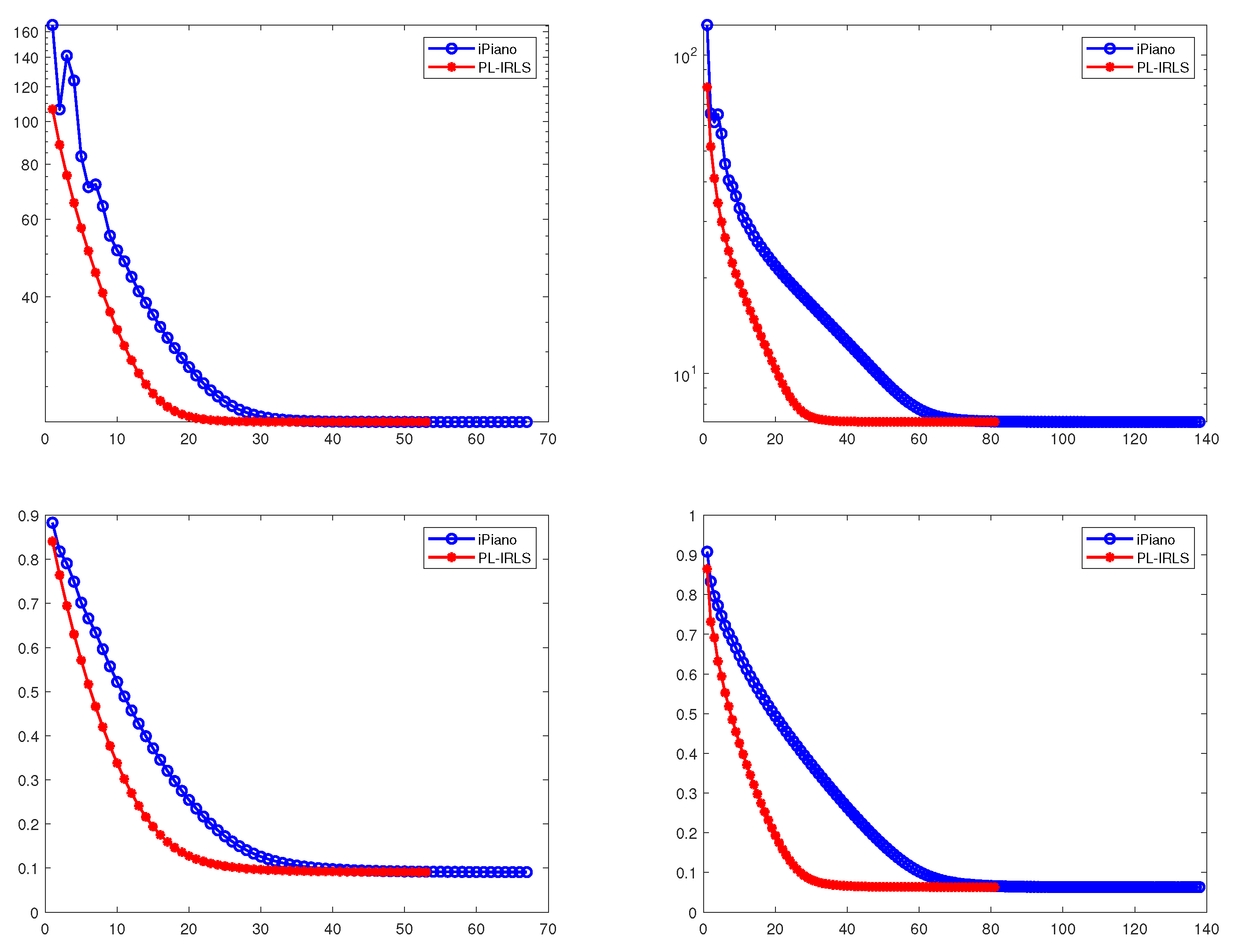
4.1. Numerical Results for PL-IRL1

First, we show the performance of PL-IRL1. The main concept of compressive sensing is that a sparse signal can be recovered from incomplete information, i.e., underdetermined system $Ax=b$ where $m\ll n$. We say that x is k-sparse if x has only k-nonzero elements. The compressive sensing problem is generally an ill-posed problem, and there exist many solutions mathematically. To obtain the sparse solution, the basic model for compressive sensing is called lasso, which has the following form:

$$\underset{x\in {\mathbb{R}}^n}{min}{\parallel x\parallel }_1+\frac{\mu }{2}{\parallel Ax-b\parallel }_2^2,$$

where $A\in {\mathbb{R}}^{m\times n}$ with $m\ll n$, $b\in {\mathbb{R}}^m$, $\mu >0$ is a positive regularization parameter. This problem is a convex relaxation of the following nonconvex ${\ell }_0$ minimization problem:

$$\underset{x\in {\mathbb{R}}^n}{min}{\parallel x\parallel }_0+\frac{\mu }{2}{\parallel Ax-b\parallel }_2^2,$$

where ${\parallel x\parallel }_0$ is defined as the number of nonzero elements of input x. Recently, sparse signal recovery from an observed signal corrupted impulsive noise was interested in lots of works [32,33,34,35]. For the sparse recovery with impulsive noise, the following ${\ell }_1$-fidelity based convex problem can be often applied:

$$\underset{x\in {\mathbb{R}}^n}{min}{\parallel x\parallel }_1+\frac{\mu }{2}{\parallel Ax-b\parallel }_1.$$

We also consider nonconvex varations of this model for a compressive sensing problem with impulsive noise as follows:

$$\underset{x\in {\mathbb{R}}^n}{min}\sum _{i=1}^n{log(1+\rho |x|}_i)+\frac{\mu }{2}{\parallel Ax-b\parallel }_1,$$

and

$$\underset{x\in {\mathbb{R}}^n}{min}\sum _{i=1}^n\frac{{\left|x\right|}_i}{1+{\rho \left|x\right|}_i}+\frac{\mu }{2}{\parallel Ax-b\parallel }_1,$$

where $\rho >0$ is a positive parameter. Unfortunately the PL-IRL1 can be directly applied to these nonconvex problems. Hence, we add the auxiliary variable $z\in {\mathbb{R}}^m$ and adopt the penalty technique, leading us to obtain the following nonconvex and nonsmooth minimization problems:

$$\underset{x\in {\mathbb{R}}^n,z\in {\mathbb{R}}^m}{min}{F}_1(x,z)=\sum _{i=1}^n{log(1+\rho |x|}_i)+\frac{\beta }{2}{\parallel z-Ax+b\parallel }_2^2+\mu {\parallel z\parallel }_1,$$

(14)

and

$$\underset{x\in {\mathbb{R}}^n,z\in {\mathbb{R}}^m}{min}{F}_2(x,z)=\sum _{i=1}^n\frac{{\left|x\right|}_i}{1+{\rho \left|x\right|}_i}+\frac{\beta }{2}{\parallel z-Ax+b\parallel }_2^2+\mu {\parallel z\parallel }_1,$$

(15)

where $\beta$ is a positive penalty constant. We set

$$\begin{array}{ccc}& & g\left(x\right)=\left|x\right|,h\left(y\right)=\mu \sum _{i=1}^{n}log(1+\rho y_i)\mathrm{or}\sum _{i=1}^n\frac{{\left|x\right|}_i}{1+{\rho \left|x\right|}_i},\hfill \\ & & f\left(x\right)=\frac{\beta }{2}{\parallel z-Ax+b\parallel }_2^2,p\left(x\right)=\frac{\mu }{2}{\parallel z\parallel }_1.\hfill \end{array}$$

In this setting, the minimization problems (14) and (15) have the form of problem (1). Since the objective function of the problem (14) is definable in the log-exp o-minimal structure, it is a KL function. The objective function of the minimization problem (15) is a semialgebraic function and it is also a KL function. Moreover, these are closed and coercive. The function f is a convex, proper and continuously differentiable function, p is a convex, proper and l.s.c function, and g is a proper and l.s.c function. The function $h:{\mathbb{R}}_{+}^n\to \mathbb{R}$ is coordinatewise nondecreasing, continuously differentiable and concave. Since the objective function involves nondifferentiable term ${\mu \parallel z\parallel }_1$, the proximal iterative reweighted algorithm proposed in [31] cannot be applied. Hence, we can apply IRL1 [10] or PL-IRL1 to solve the given problem (14). The IRL1 or PL-IRL1 applied to the problem (14) is given as follows:

$$\left\{\begin{array}{ccc}{\displaystyle w^k}\hfill & =\hfill & {\displaystyle \left\{\begin{array}{cc}{\displaystyle \frac{\rho }{1+\rho |x^k|}}\hfill & \mathrm{for}\left(14\right)\hfill \\ {\displaystyle \frac{1}{(1+\rho |x^k{\left|\right)}^2}}\hfill & \mathrm{for}\left(15\right)\hfill \end{array}\right.,}\hfill \\ {\displaystyle (x^{k+1},z^{k+1})}\hfill & =\hfill & {\displaystyle arg\underset{x,z}{min}\langle w^k,\left|x\right|\rangle +\frac{\beta }{2}{\parallel z-Ax+b\parallel }_2^2+\mu {\parallel z\parallel }_1,}\hfill \end{array}\right.$$

(16)

and

$$\left\{\begin{array}{ccc}{\displaystyle w^k}\hfill & =\hfill & {\displaystyle \left\{\begin{array}{cc}{\displaystyle \frac{\rho }{1+\rho |x^k|}}\hfill & \mathrm{for}\left(14\right)\hfill \\ {\displaystyle \frac{1}{(1+\rho |x^k{\left|\right)}^2}}\hfill & \mathrm{for}\left(15\right)\hfill \end{array}\right.,}\hfill \\ {\displaystyle (x^{k+1},z^{k+1})}\hfill & =\hfill & {\displaystyle arg\underset{x,z}{min}\langle w^k,\left|x\right|\rangle +\beta \langle z^k-A{x}^k+b,z-Ax+b\rangle +\mu {\parallel z\parallel }_1}\hfill \\ \hfill & \hfill & +\frac{\delta }{2}\parallel x-x^k{\parallel }_2^2+\frac{\delta }{2}{\parallel z-z^k\parallel }_2^2,\hfill \end{array}\right.$$

(17)

respectively. For solving the convex subproblem of IRL1, the optimality conditions are given as follows:

$$\left\{\begin{array}{ccc}{\displaystyle 0}\hfill & \in \hfill & \partial (\langle w^k,\left|x\right|\rangle )\left(x^{k+1}\right)+\beta A^T(A{x}^{k+1}-b-z^{k+1}),\hfill \\ {\displaystyle 0}\hfill & \in \hfill & \beta (z^{k+1}-A{x}^{k+1}+b)+{\mu \partial (\parallel z\parallel }_1)\left(z^{k+1}\right).\hfill \end{array}\right.$$

(18)

This system (18) of equations does not have a closed form solution. Hence, the IRL1 cannot be employed to solve the problem (14). On the other hand, the optimality conditions of the convex subproblem of our method are given as

$$\left\{\begin{array}{ccc}{\displaystyle 0}\hfill & \in \hfill & \partial (\langle w^k,\left|x\right|\rangle )\left(x^{k+1}\right)+\beta A^T(A{x}^k-b-z^k)+\delta (x^{k+1}-x^k),\hfill \\ {\displaystyle 0}\hfill & \in \hfill & \beta (z^k-A{x}^k+b)+{\mu (\parallel z\parallel }_1)\left(z^{k+1}\right)+\delta (z^{k+1}-z^k).\hfill \end{array}\right.$$

(19)

These equations in (19) are separable, and each problem has a closed form solution:

$$\begin{array}{ccc}\hfill x^{k+1}& =& \mathrm{shrink}\left(x^k-\frac{\beta }{\delta }{A}^T(A{x}^k-b-z^k),\frac{w^k}{\delta }\right),\hfill \\ \hfill z^{k+1}& =& \mathrm{shrink}\left(z^k-\frac{\beta }{\delta }(z^k-A{x}^k+b),\frac{\mu }{\delta }\right),\hfill \end{array}$$

where shrink function is defined as

$$\mathrm{shrink}(a,b)=\mathrm{sign}\left(a\right)·max\left(\right|a|-b,0).$$

To show the convergence of the PL-IRL1 to solve problems (14) and (15), we perform the numerical experiments in the following setting. The size of A is $n=5000$ and $m=2500$. We use an orthonormal Gaussian measurement matrix A whose entries are randomly chosen by standard Gaussian distribution, and then each column of A is divided by its ${\ell }_2$ norm. The number l of nonzero elements of the original sparse signal $x_0$ is fixed at 50, the locations of nonzero elements are selected randomly, and the values of nonzero elements are chosen by Gaussian distribution $\mathcal{N}(0,{10}^2)$. The observed data b can be calculated by

$$b=A{x}_0+n,$$

where n is the Gaussian mixture noise that consists of two Gaussian components, which is one of impulsive noise in signal processing [36]. The measured equation of n is given by

$$n=\nu n_1+(1-\nu )n_2,$$

where $n_1$ and $n_2$ are Gaussian noise with mean 0 and standard deviation $\eta$ and $q\eta$. The $n_1$ denotes the background noise, and $n_1$ represents the influence of outliers. The parameter $\nu \in (0,1)$ controls the proportion of the large outliers and $q>1$ controls the strength of the outliers. Here, we fixed these parameters at $(\nu ,q,\eta )=(0.1,\sqrt{10},0.02)$.

Since ${\parallel A\parallel }_2=1$, the Lipschitz constant of $\nabla f$ is $2\beta$. So, $\delta$ is set to be $\beta +0.001$. The regularization parameter $\mu$ is fixed at $0.2$ for (14) or $1.5$ for (15); the penalty parameter $\beta$ is set to be 2 for (14) or 28 for (15); and the controlling parameter $\rho$ of nonconvexity is set to be $0.1$. For the stopping condition of our algorithm, we use relative errors over energy function values, whose specific formulation is given as

$$\frac{F_i\left(x^k\right)-F_i\left(x^{k+1}\right)}{F_i\left(x^0\right)}<{10}^{-7},i=1,2.$$

For this setting, 100 different numerical tests are conducted.

In

Table 1. Numerical results for PL-IRL1 algorithm applied to models (14) and (15).

Model		Computing Time (s)	Iterations	Energy	Relative Error
Problem (14)	mean	5.437452	142	34.1832	$3.5502\times {10}^{-2}$
	std	0.293790	8	2.1721	$4.5748\times {10}^{-3}$
Problem (15)	mean	8.960141	236	282.1852	$3.1598\times {10}^{-2}$
	std	0.563042	15	13.0279	$4.2781\times {10}^{-3}$

, we present the computing time, number of iterations, final energy value, and relative error. From the relative errors, we can observe that the proposed algorithm finds an approximated sparse solution with small error for all cases. In Figure 1, we illustrate the relative errors and energy values $F_i\left(x^k\right)$ over k iterations. Since the penalty parameter $\beta$ for (14) is smaller than that for (15), the computing time of our method for solving (14) is faster than that for solving (15). We can also see similar results in terms of the number of iterations. Ultimately, we can show in Figure 1 and Table 1 the fast convergence of the PL-IRL1, and the final energy value has enough small value.

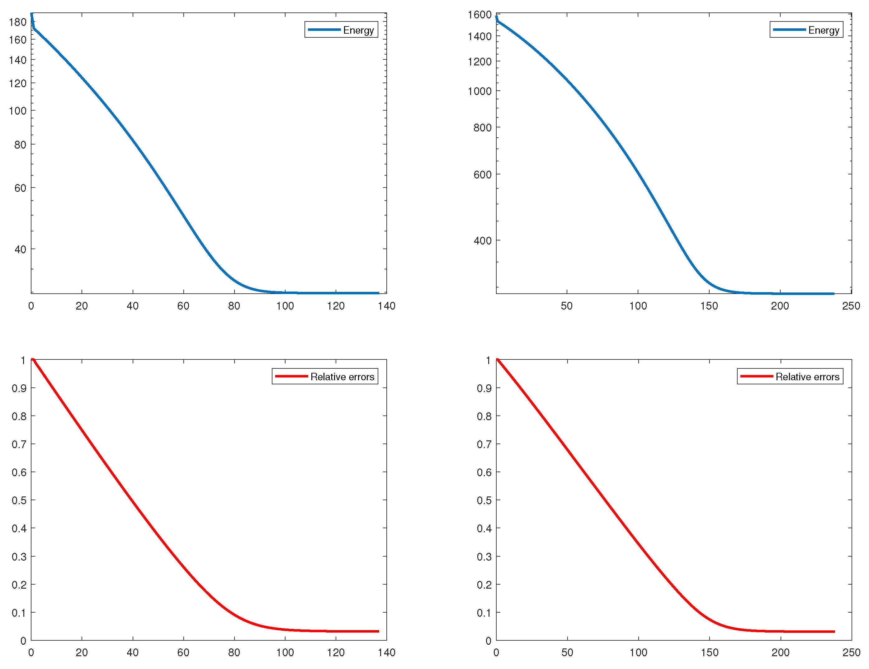
4.2. Numerical Results for PL-IRLS

Second, we present numerical results of PL-IRLS compared with the iPiano [17] method for the compressive sensing problem in signal processing. Specifically, the restoration of the sparse signal corrupted by additive Gaussian noise is considered. We apply the algorithms PL-IRLS and iPiano to the following unconstrained problems:

$$\underset{x\in {\mathbb{R}}^n}{min}\frac{1}{2\rho }\sum _{i=1}^n{log(1+\rho |x|}_i^2)+\frac{\beta }{2}{\parallel x\parallel }_2^2+\frac{\mu }{2}{\parallel Ax-b\parallel }_2^2,$$

(20)

and

$$\underset{x\in {\mathbb{R}}^n}{min}\frac{1}{2}\sum _{i=1}^n\frac{{\left|x\right|}_i^2}{1+{\rho \left(\right|x|}_i{+c)}^2}+\frac{\beta }{2}{\parallel x\parallel }_2^2+\frac{\mu }{2}{\parallel Ax-b\parallel }_2^2,$$

(21)

where $\beta ,\mu$ are positive parameters, c is a positive constant, and $\rho >0$ is the parameter that controls the nonconvexity of regularizing term. These problems are a nonconvex variations of lasso, which is a well-known model for compressive sensing. The objective functions of problems (20) and (21) are definable in the log-exp o-minimal structure, and they are also close, coercive KL functions. With setting

$$\begin{array}{ccc}& & g\left(x\right)=\left|x\right|,h\left(y\right)=\frac{1}{2\rho }\sum _{i=1}^{n}log(1+\rho y_i^2)\mathrm{or}\frac{1}{2}\sum _{i=1}^n\frac{y_i^2}{1+\rho {(y_i+c)}^2}\hfill \\ & & f\left(x\right)=\frac{\mu }{2}{\parallel Ax-b\parallel }_2^2,p\left(x\right)=\frac{\beta }{2}{\parallel x\parallel }_2^2,\hfill \end{array}$$

all assumptions in Algorithm 4 are satisfied. Since the norm of the Hessian matrix of h is bounded on ${\mathbb{R}}_{+}^n$, it has also a strictly continuous gradient. The PL-IRLS applied to the problems (20) and (21) can be obtained by

$$\left\{\begin{array}{ccc}{\displaystyle w^k}\hfill & =\hfill & {\displaystyle \left\{\begin{array}{cc}{\displaystyle \frac{1}{1+\rho |x^k{|}^2},}\hfill & \mathrm{for}\left(20\right)\hfill \\ {\displaystyle \frac{c\rho \left(\right|x^k|+c)+1}{(1+\rho (|x^k{|+c))}^2}}\hfill & \mathrm{for}\left(21\right)\hfill \end{array}\right.,}\hfill \\ {\displaystyle x^{k+1}}\hfill & =\hfill & {\displaystyle arg\underset{x}{min}\frac{1}{2}\langle w^k,x^2\rangle +\frac{\delta }{2}{\parallel x-x^k\parallel }_2^2+\mu \langle A^T(A{x}^k-b),x-x^k\rangle .}\hfill \end{array}\right.$$

(22)

The subproblem in (22) is a quadratic problem, and its normal equation is given as follows:

$$w^{k}x+\delta (x-x^k)+\mu A^T(A{x}^k-b)=0.$$

It can be rewritten as the following linear equation,

$$(diag\left(w^k\right)+\delta I)x=\delta x^k-\mu A^T(A{x}^k-b),$$

where $diag\left(w^k\right)$ is a diagonal matrix whose diagonal entries consist of $w^k$. Since $diag\left(w^k\right)+\delta I$ is a diagonal matrix, this linear equation can be solved exactly and easily. The majorization property of PL-IRLS is obtained from ([10], Proposition 23) for any $\rho >0$ and $c>0$.

In this experiment, we use partial discrete cosine transform (DCT) matrices A whose i-th rows are selected from the $n\times n$ DCT matrix. We note that the partial DCT matrices are implicitly stored, i.e., matrix-vector multiplications in $Ax$ or $A^{T}x$ are computed by the DCT or inverse of DCT. Hence, we can use partial DCT matrices of very large sizes. Here, the size $n,m$ is fixed at $(n,m)$ = (100,000, 30,000). Then, the original IRLS can be actually applied to the nonsmooth and nonconvex problem (20), which is given by

$$\left\{\begin{array}{ccc}{\displaystyle w^k}\hfill & =\hfill & {\displaystyle \left\{\begin{array}{cc}{\displaystyle \frac{1}{1+\rho |x^k{|}^2},}\hfill & \mathrm{for}\left(20\right)\hfill \\ {\displaystyle \frac{c\rho \left(\right|x^k|+c)+1}{(1+\rho (|x^k{|+c))}^2}}\hfill & \mathrm{for}\left(21\right)\hfill \end{array}\right.,}\hfill \\ {\displaystyle x^{k+1}}\hfill & =\hfill & {\displaystyle arg\underset{x}{min}\frac{1}{2}\langle w^k,x^2\rangle +\frac{\mu }{2}{\parallel Ax-b\parallel }_2^2.}\hfill \end{array}\right.$$

(23)

The optimality condition of the subproblem in the method (23) is

$$w^k{x}^{k+1}+\mu A^T(A{x}^{k+1}-b)=0,$$

and it is equivalent to

$$(diag\left(w^k\right)+\mu A^{T}A)x^{k+1}=\mu A^{T}b.$$

Since the size of our measurement matrix is very large, finding the exact solution of this linear equation is time consuming and it seem to be impossible in many cases.

The number l of nonzero elements of the sparse signal $x_0$ is fixed at 2000, and the locations of nonzero elements are randomly chosen. The values of nonzero elements are selected from standard Gaussian distribution. The observed data b is measured by the formula

$$b=A{x}_0+n,$$

where n is the Gaussian white noise with mean 0 and standard deviation 0.02. The regularization parameters $(\beta ,\mu )$ are fixed at $(0.001,1.5)$ for (20) or $(0.001,0.9)$ for (21) in all tests. The values of $(\rho ,c)$ are also fixed at $(250,0.001)$. The proximity parameter $\delta$ in our method is set to be $\frac{\mu }{2}+0.0001$ because the ${\ell }_2$ norm of a partial DCT matrix is less than or equal to 1.

We present the mean values and standard deviations over 100 trials of computing time, number of iterations, energy value and relative error in

Table 2. Numerical results for PL-IRL1 and iPiano applied to the model (20) and (21).

Method		Computing Time (s)	Iterations	Energy	Relative Error
Model (20)
PL-IRLS	mean	3.255264	53	21.2322	$8.7822\times {10}^{-2}$
	std	0.215043	1	0.2123	$2.0949\times {10}^{-3}$
iPiano	mean	4.165273	68	21.2323	$8.7787\times {10}^{-2}$
	std	0.226674	1	0.2123	$2.0945\times {10}^{-3}$
Model (21)
PL-IRLS	mean	5.588428	90	7.1838	$6.1408\times {10}^{-2}$
	std	0.775879	11	0.0483	$1.4041\times {10}^{-3}$
iPiano	mean	8.849843	144	7.1840	$6.1389\times {10}^{-2}$
	std	0.915589	12	0.0483	$1.4009\times {10}^{-3}$

. In Figure 2, we plot the relative errors and energy values of PL-IRLS and iPiano over iterations. Figure 2 shows the convergence of PL-IRLS and iPiano. For the tests, average values of the energy value and relative error for PL-IRLS are almost same with those for the iPiano. This shows that PL-IRLS and iPiano recover almost the same sparse solutions. Hence, it demonstrates the similar performance between PL-IRLS and iPiano in terms of the accuracy and optimization of energy functional. On the other hand, it can be observed in Table 2 and Figure 2 that PL-IRLS is faster than iPiano. Therefore, PL-IRLS is superior to iPiano for solving the nonconvex and nonsmooth problems (20) and (21). In conclusion, PL-IRLS gives better performance over iPiano.

5. Conclusions

In this paper, we proposed proximal linearized reweighted algorithms to solve nonconvex and nonsmooth unconstrained minimization problem (1). Based on the general unified framework, we suggested an extension of the iterative convex majorization–minimization method for solving (1). Moreover, extended versions of the iteratively reweighted ${\ell }_1$ algorithm and iterative least square algorithm were also introduced. The global convergence of the proposed algorithm was also proved under uncertain assumptions. Lastly, the numerical results related to compressive sensing demonstrated that the proposed methods provides the outstanding performance compared with state-of-the-art methods. Recently, several algorithms were extended by imposing an additional inertial term, resulting in a faster convergence rate. In future, we will study a proximal linearized reweighted algorithm with an inertial force.

References

1. Curry, H.B. The method of steepest descent for non-linear minimization problems. Q. Appl. Math. 1944, 2, 258–261. [Google Scholar] [CrossRef] [Green Version]
2. Nesterov, Y.E. A method for solving the convex programming problem with convergence rate O ( 1 / k 2 ^ ) . Dokl. Akad. Nauk Sssr 1983, 269, 543–547. [Google Scholar]
3. Beck, A.; Teboulle, M. A fast iterative shrinkage-thresholding algorithm for linear inverse problems. SIAM J. Imaging Sci. 2009, 2, 183–202. [Google Scholar] [CrossRef] [Green Version]
4. Rockafellar, R.T. Monotone operators and the proximal point algorithm. SIAM J. Control Optim. 1976, 14, 877–898. [Google Scholar] [CrossRef] [Green Version]
5. Kaplan, A.; Tichatschke, R. Proximal point methods and nonconvex optimization. J. Glob. Optim. 1998, 13, 389–406. [Google Scholar] [CrossRef]
6. Gong, P.; Zhang, C.; Lu, Z.; Huang, J.; Ye, J. A general iterative shrinkage and thresholding algorithm for non-convex regularized optimization problems. In Proceedings of the 30th International Conference on Machine Learning. PMLR 2013, 28, 37–45. [Google Scholar]
7. Attouch, H.; Bolte, J.; Redont, P.; Soubeyran, A. Proximal alternating minimization and projection methods for nonconvex problems: An approach based on the Kurdyka-Łojasiewicz inequality. Math. Oper. Res. 2010, 35, 438–457. [Google Scholar] [CrossRef] [Green Version]
8. Candes, E.J.; Wakin, M.B.; Boyd, S.P. Enhancing sparsity by reweighted 1 minimization. J. Fourier Anal. Appl. 2008, 14, 877–905. [Google Scholar] [CrossRef]
9. Lai, M.J.; Xu, Y.; Yin, W. Improved iteratively reweighted least squares for unconstrained smoothed q minimization. SIAM J. Numer. Anal. 2013, 51, 927–957. [Google Scholar] [CrossRef]
10. Ochs, P.; Dosovitskiy, A.; Brox, T.; Pock, T. On iteratively reweighted algorithms for nonsmooth nonconvex optimization in computer vision. SIAM J. Imaging Sci. 2015, 8, 331–372. [Google Scholar] [CrossRef]
11. Łojasiewicz, S. Sur la géométrie semi-et sous-analytique. Ann. l’Institut Fourier 1993, 43, 1575–1595. [Google Scholar] [CrossRef]
12. Łojasiewicz, S. Une propriété topologique des sous-ensembles analytiques réels. Les Équations aux Dérivées Partielles 1963, 117, 87–89. [Google Scholar]
13. Bolte, J.; Daniilidis, A.; Lewis, A.; Shiota, M. Clarke subgradients of stratifiable functions. SIAM J. Optim. 2007, 18, 556–572. [Google Scholar] [CrossRef] [Green Version]
14. Bolte, J.; Daniilidis, A.; Lewis, A. The Lojasiewicz inequality for nonsmooth subanalytic functions with applications to subgradient dynamical systems. SIAM J. Optim. 2007, 17, 1205–1223. [Google Scholar] [CrossRef]
15. Bolte, J.; Combettes, P.L.; Pesquet, J.C. Alternating proximal algorithm for blind image recovery. In Proceedings of the 2010 IEEE International Conference on Image Processing, Hong Kong, China, 26–29 September 2010; pp. 1673–1676. [Google Scholar] [CrossRef] [Green Version]
16. Attouch, H.; Bolte, J. On the convergence of the proximal algorithm for nonsmooth functions involving analytic features. Math. Program. 2009, 116, 5–16. [Google Scholar] [CrossRef]
17. Ochs, P.; Chen, Y.; Brox, T.; Pock, T. iPiano: Inertial proximal algorithm for nonconvex optimization. SIAM J. Imaging Sci. 2014, 7, 1388–1419. [Google Scholar] [CrossRef]
18. Attouch, H.; Bolte, J.; Svaiter, B.F. Convergence of descent methods for semi-algebraic and tame problems: Proximal algorithms, forward–backward splitting, and regularized Gauss–Seidel methods. Math. Program. 2013, 137, 91–129. [Google Scholar] [CrossRef]
19. Osher, S.; Mao, Y.; Dong, B.; Yin, W. Fast linearized Bregman iteration for compressive sensing and sparse denoising. Commun. Math. Sci. 2010, 8, 93–111. [Google Scholar]
20. Bolte, J.; Sabach, S.; Teboulle, M. Proximal alternating linearized minimization for nonconvex and nonsmooth problems. Math. Program. 2014, 146, 459–494. [Google Scholar] [CrossRef]
21. Rockafellar, R.T.; Wets, R.J.B. Variational Analysis; Springer Science & Business Media: Berlin/Heidelberg, Germany, 2009; Volume 317. [Google Scholar]
22. Mordukhovich, B.S.; Nam, N.M.; Yen, N. Fréchet subdifferential calculus and optimality conditions in nondifferentiable programming. Optimization 2006, 55, 685–708. [Google Scholar] [CrossRef] [Green Version]
23. Bochnak, J.; Coste, M.; Roy, M.F. Real Algebraic Geometry; Springer Science & Business Media: Berlin/Heidelberg, Germany, 2013; Volume 36. [Google Scholar]
24. Wilkie, A.J. Model completeness results for expansions of the ordered field of real numbers by restricted Pfaffian functions and the exponential function. J. Am. Math. Soc. 1996, 9, 1051–1094. [Google Scholar] [CrossRef]
25. Dries, L.P.D.v.d. Tame Topology and O-Minimal Structures; Cambridge University Press: Cambridge, UK, 1998; Volume 248. [Google Scholar]
26. Kang, M. Approximate versions of proximal iteratively reweighted algorithms including an extended IP-ICMM for signal and image processing problems. J. Comput. Appl. Math. 2020, 376, 112837. [Google Scholar] [CrossRef]
27. Combettes, P.L.; Wajs, V.R. Signal recovery by proximal forward-backward splitting. Multiscale Model. Simul. 2005, 4, 1168–1200. [Google Scholar] [CrossRef] [Green Version]
28. Chartrand, R.; Yin, W. Iteratively reweighted algorithms for compressive sensing. In Proceedings of the 2008 IEEE International Conference on Acoustics, Speech and Signal Processing, Las Vegas, NV, USA, 31 March–4 April 2008; pp. 3869–3872. [Google Scholar]
29. Daubechies, I.; DeVore, R.; Fornasier, M.; Güntürk, C.S. Iteratively reweighted least squares minimization for sparse recovery. Commun. Pure Appl. Math. 2010, 63, 1–38. [Google Scholar] [CrossRef] [Green Version]
30. Needell, D. Noisy signal recovery via iterative reweighted L1-minimization. In Proceedings of the 2009 Conference Record of the Forty-Third Asilomar Conference on Signals, Systems and Computers, Pacific Grove, CA, USA, 1–4 November 2009; pp. 113–117. [Google Scholar]
31. Sun, T.; Jiang, H.; Cheng, L. Global convergence of proximal iteratively reweighted algorithm. J. Glob. Optim. 2017, 68, 815–826. [Google Scholar] [CrossRef]
32. Ji, Y.; Yang, Z.; Li, W. Bayesian sparse reconstruction method of compressed sensing in the presence of impulsive noise. Circuits Syst. Signal Process. 2013, 32, 2971–2998. [Google Scholar] [CrossRef]
33. Javaheri, A.; Zayyani, H.; Figueiredo, M.A.; Marvasti, F. Robust sparse recovery in impulsive noise via continuous mixed norm. IEEE Signal Process. Lett. 2018, 25, 1146–1150. [Google Scholar] [CrossRef]
34. Wen, F.; Liu, P.; Liu, Y.; Qiu, R.C.; Yu, W. Robust Sparse Recovery in Impulsive Noise via p-1 Optimization. IEEE Trans. Signal Process. 2016, 65, 105–118. [Google Scholar] [CrossRef]
35. Wen, J.; Weng, J.; Tong, C.; Ren, C.; Zhou, Z. Sparse signal recovery with minimization of 1-norm minus 2-norm. IEEE Trans. Veh. Technol. 2019, 68, 6847–6854. [Google Scholar] [CrossRef]
36. Wen, F.; Pei, L.; Yang, Y.; Yu, W.; Liu, P. Efficient and robust recovery of sparse signal and image using generalized nonconvex regularization. IEEE Trans. Comput. Imaging 2017, 3, 566–579. [Google Scholar] [CrossRef] [Green Version]
Figure 1. Comparison results of the energy and relative error for PL-IRL1 algorithm applied to problems (14) and (15). Left: Result for problem (14). Right: Result for problem (15).
Axioms 11 00201 g001
Figure 2. Comparison results of the energy and relative errors for PL-IRLS and iPiano applied to problem (20) and (21). Left: Result for problem (20). Right: Result for problem (21).
Axioms 11 00201 g002