
The Boundary Value Problem with Stationary Inhomogeneities for a Hyperbolic-Type Equation with a Fractional Derivative

Abstract
:1. Introduction
2. Problem Statement and Solution Method
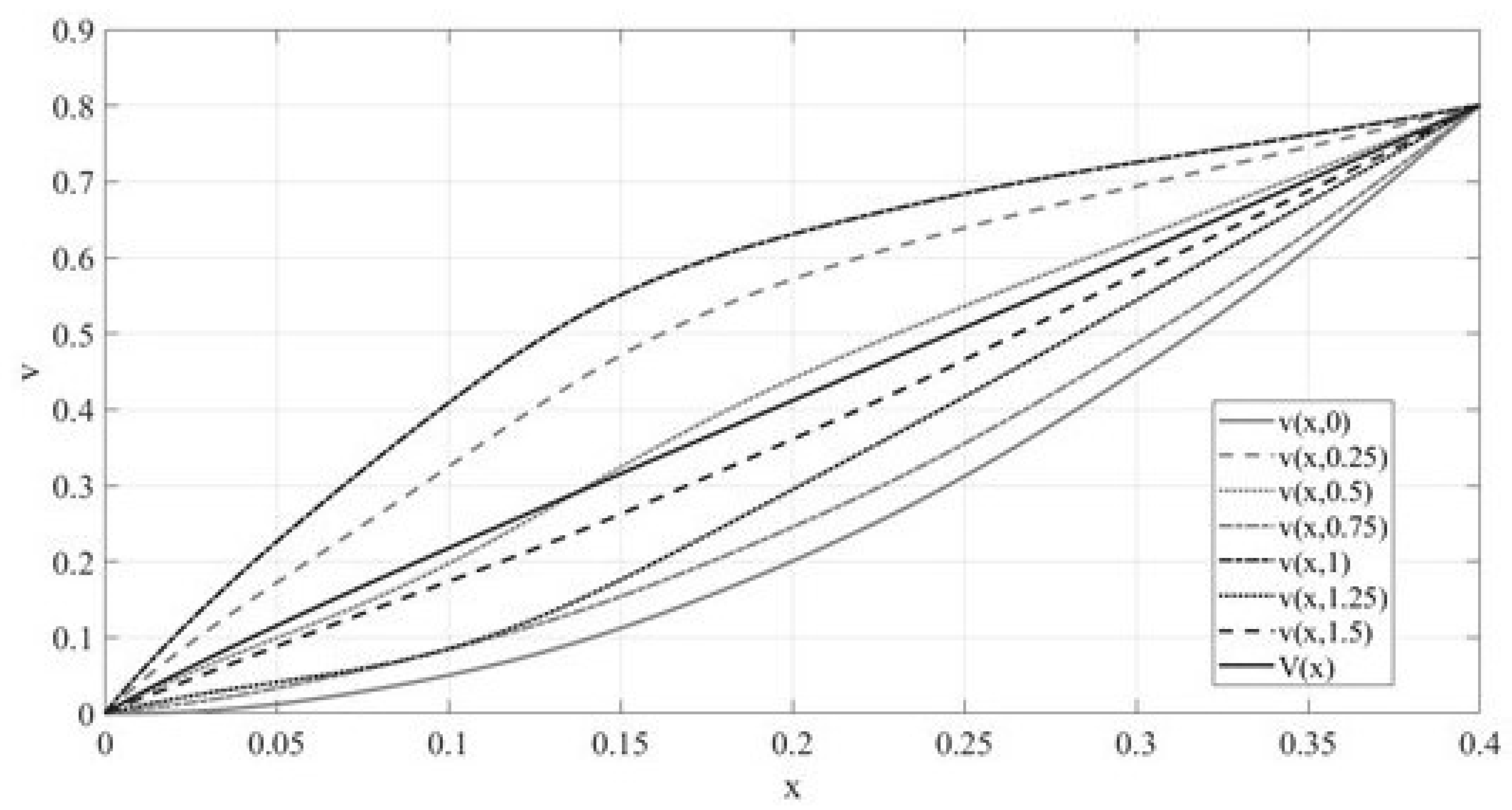
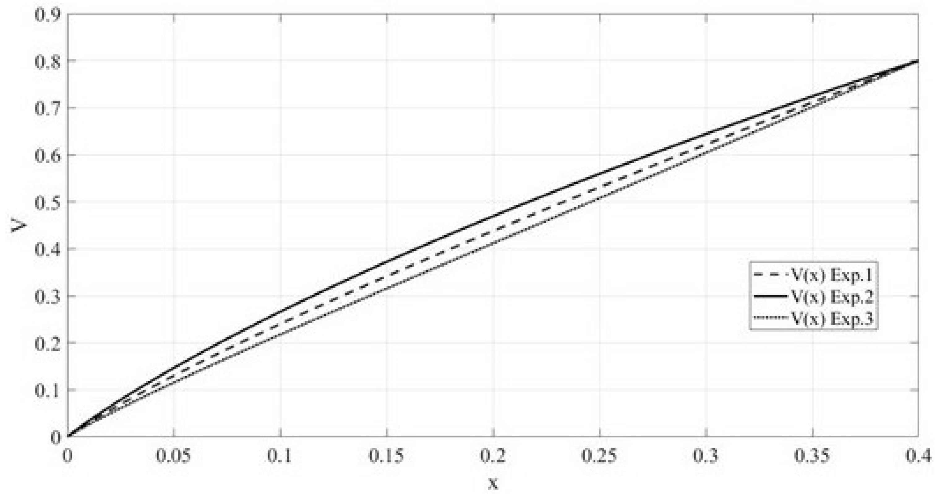
3. Results
4. Discussion
Funding
Data Availability Statement
Acknowledgments
Conflicts of Interest
References
- Machado, J.A.T. (Ed.) Handbook of Fractional Calculus with Applications; De Gruyter GmbH: Berlin, Germany; Boston, MA, USA, 2019; Volumes 1–8. [Google Scholar]
- Aleroev, T.S.; Zveryayev, E.M.; Larionov, E.A. Fractional calculus and its application. Preprinty IPM im. M.V. Keldysha [KIAM Preprint] 2013, 37, 25. [Google Scholar]
- Sabatier, J.; Agrawal, O.; Machado, A. Advances in Fractional Calculus. In Theoretical Developments and Applications in Physics and Engineering; Springer: Dordrecht, The Netherlands, 2007. [Google Scholar]
- Aleroev, T.; Aleroeva, H.; Huang, J.; Nie, N.; Tang, Y.; Zhang, Y. Features of seepage of a liquid to a chink in the cracked deformable layer. Int. J. Model. Simul. Sci. Comput. 2010, 1, 333–347. [Google Scholar] [CrossRef]
- Herrmann, R. Fractional Calculus: An Introduction for Physicists, 2nd ed.; World Scientific: Singapore, 2014. [Google Scholar]
- Sandev, T.; Tomovshi, Z. Fractional Equations and Models: Theory and Applications; Springer: Berlin, Germany, 2019. [Google Scholar]
- Sabattelli, L.; Keating, S.; Dudley, J.; Richmond, P. Waiting time distributions in financial markets. Eur. Phys. J. B 2002, 27, 273–275. [Google Scholar] [CrossRef]
- Song, L.; Wang, W. Solution of the fractional Black-Scholes option pricing model by finite difference method. Abstr. Appl. Anal 2013, 45, 1–16. [Google Scholar] [CrossRef] [Green Version]
- Magin, R. Fractional Calculus in Bioengineering; Begell House Publishers: Danbury, CT, USA, 2006. [Google Scholar]
- Yuste, S.; Lindenberg, K. Subdiffusion-limited reactions. Chem. Phys. 2002, 284, 169–180. [Google Scholar] [CrossRef] [Green Version]
- Kirianova, L. Modeling of Strength Characteristics of Polymer Concrete Via the Wave Equation with a Fractional Derivative. Mathematics 2020, 8, 1843. [Google Scholar] [CrossRef]
- Samarskiy, A.A.; Tikhonov, A.N. Equations of Mathematical Physics, 6th ed.; Publishing house of Moscow State University: Moscow, Russia, 1999. [Google Scholar]
- Dzhrbashyan, M.M. Integral Transformations and Representations of Functions in a Complex Area; Nauka: Moscow, Russia, 1966. [Google Scholar]
- Aleroev, T.; Erokhin, S.; Kekharsaeva, E. Modeling of deformation-strength characteristics of polymer concrete using fractional calculus. Iop Mater. Sci. Eng. 2018, 365, 032004. [Google Scholar] [CrossRef] [Green Version]
- Kekharsaeva, E.R.; Pirozhkov, V.G. Mekhanika Kompozitsionnykh Materialov i Konstruktsii, Slozhnykh i Geterogennykh Sred; IPRIM RAN: Moscow, Russia, 2016. [Google Scholar]
- Kirianova, L. The fractional derivative type identification for the modelling deformation and strength characteristics of polymer concrete. Iop Conf. Ser. Mater. Sci. Eng. 2021, 1030, 012094. [Google Scholar] [CrossRef]
- Aleroev, T.; Kirianova, L. Presence of Basic Oscillatory Properties in the Bagley-Torvik Model. In IPICSE-2018 MATEC Web of Conferences; EDP Sciences: Les Ulis, France, 2018; Volume 251, p. 04022. [Google Scholar]
- Zhang, J.; Aleroev, T.; Tang, Y.; Huang, J. Numerical Schemes for Time-Space Fractional Vibration Equations. Adv. Appl. Math. Mech. 2021, 13, 806–826. [Google Scholar]
- Elsayed, A.M.; Orlov, V.N. Numerical Scheme for Solving Time–Space Vibration String Equation of Fractional Derivative. Mathematics 2020, 8, 1069. [Google Scholar] [CrossRef]

| Designation | Values |
|---|---|
| 85.95 | |
| 319.99 | |
| 689.11 | |
| 1192.21 | |
| 1826.89 | |
| 2592.81 | |
| 3488.83 |
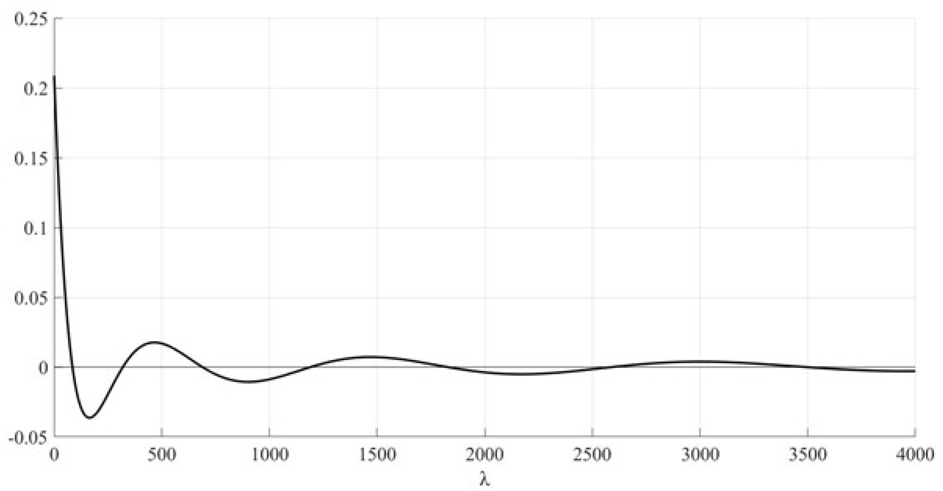
| k | |
|---|---|
| 1 | 0.001162 |
| 2 | −0.000245 |
| 3 | 0.000096 |
| 4 | −0.000047 |
| 5 | 0.000027 |
| 6 | −0.000017 |
| 7 | 0.000011 |
Publisher’s Note: MDPI stays neutral with regard to jurisdictional claims in published maps and institutional affiliations. |
© 2022 by the author. Licensee MDPI, Basel, Switzerland. This article is an open access article distributed under the terms and conditions of the Creative Commons Attribution (CC BY) license (https://creativecommons.org/licenses/by/4.0/).
Share and Cite
Kirianova, L.V. The Boundary Value Problem with Stationary Inhomogeneities for a Hyperbolic-Type Equation with a Fractional Derivative. Axioms 2022, 11, 207. https://doi.org/10.3390/axioms11050207
Kirianova LV. The Boundary Value Problem with Stationary Inhomogeneities for a Hyperbolic-Type Equation with a Fractional Derivative. Axioms. 2022; 11(5):207. https://doi.org/10.3390/axioms11050207
Chicago/Turabian StyleKirianova, Ludmila Vladimirovna. 2022. "The Boundary Value Problem with Stationary Inhomogeneities for a Hyperbolic-Type Equation with a Fractional Derivative" Axioms 11, no. 5: 207. https://doi.org/10.3390/axioms11050207