Abstract
With the popularity of big data analysis with insurance claim count data, diverse regression models for count response variable have been developed. However, there is a multicollinearlity issue with multivariate input variables to the count response regression models. Recently, deep learning and neural network models for count response have been proposed, and a Keras and Tensorflow-based deep learning model has been also proposed. To apply the deep learning and neural network models to non-normal insurance claim count data, we perform the root mean square error accuracy comparison of gradient boosting machines (a popular machine learning regression tree algorithm), principal component analysis (PCA)-based Poisson regression, PCA-based negative binomial regression, and PCA-based zero inflated poisson regression to avoid the multicollinearity of multivariate input variables with the simulated normal distribution data and the non-normal simulated data combined with normally distributed data, binary data, copula-based asymmetrical data, and two real data sets, which consist of speeding ticket and Singapore insurance claim count data.
MSC:
62P05
1. Introduction
Since 2019, the news has provided people with information about COVID-19 (Coronavirus disease 2019). In an effort to protect people from COVID-19, researchers have studied the relationship between the number of COVID-19 patients (i.e., patients with a confirmed COVID-19 infection) in their country and their government’s policies related to COVID-19, such as restrictions on international air travel and closures of institutions. The analysis of medical data using machine learning methods could potentially be useful in understanding how to protect people from COVID-19. An example of the usefulness of machine learning methods is extracting information from the data produced from social media platforms. Deep learning (DL) has provided useful results in predicting problems for a variety of fields [1,2]. In particular, the core architectures that currently dominate DL are autoencoders, convolutional neural networks, deep feed-forward neural networks, generative adversarial networks, long short-term memory networks, and recurrent neural networks.
It has been interesting to study DL from a statistical perspective [3,4]. Standard statistical models such as the Poisson generalized linear model (GLM) and Cox’s proportional hazards (PH) model have been applied to the DL models [5,6].
The DL model can be regarded as a highly nonlinear and generalized non-parametric function form including the traditional statistical models. In particular, the feed-forward DL model can be viewed as a stacked GLM with recursively defined nonlinear link functions [7,8]. Machine learning techniques have generated actionable intelligence for the manufacturing industry through the processing of big data [9], which has helped in increasing manufacturing efficiency without requiring significant changes. Machine learning to statistical process control (SPC) for count or binary response data has been developed to improve the quality of products and reduce process variations [10,11,12,13,14,15]. The principal component analysis (PCA)-based Poisson, negative binomial and COM-Poisson r-control charts for monitoring dispersed count data to avoid multicollinearity have been proposed by [14,15]. The deep learning and neural network-based residual control charts for the binary asymmetrical response variable with highly correlated multivariate covariates have been outperformed by PCA-based GLM with probit, PCA-based GLM with logit, nonlinear PCA-based GLM with probit, and nonlinear PCA-based GLM with logit [11,12]. Based on the results of [11,12], the deep learning (DL) and neural network (NN) residual control charts for the count response regression model to monitor the asymmetrical and dispersed count response data have been proposed by [16]. Meanwhile, Kim and Ha’s DL residual control chart outperformed PCA-based Poisson, PCA-based negative binomial, nonlinear PCA-based Poisson, and nonlinear PCA-based negative binomial in terms of accuracy [16].
Recently, several NN and DL models for analyzing count data, including insurance claim data, have been studied [17,18,19,20,21,22]. However, these researchers did not investigate the behaviors of network models allowing for correlated and/or non-normal input variables. A multilayer deep neural network (DLk) survival model using Keras and Tensorflow has been proposed by [5].
In this paper, we also consider an important class of machine learning algorithms featuring a tree-based ensemble method including gradient boosting machines (GBM). The GBM is a machine learning technique used in regression and classification tasks, among others. It generates a final prediction model in the form of an ensemble of weak prediction models, which are multiple decision trees. In this research, we want to compare DL and NN models with the DLk model, GBM, PCA-based Poisson regression (POI), PCA-based negative binomial regression (NB), and PCA-based zero-inflated Poisson regression (ZIP) when the high correlated multivariate input variables follow nonlinear and non-normal distributions.
DL and NN models for the asymmetrical count response variable with highly correlated covariates will be applied to simulated, highly correlated multivariate normal and non-normal data generated by copula functions, real speeding ticket data and real insurance claim data. This paper is organized as follows: Section 2 reviews the statistical regression models and DL models for count data methods. In Section 3, we compare DL and NN with DLk, GBM, POI, ZIP, and NB using simulated non-normal data generated by copula functions. Section 4 also compares DL and NN with DLk, GBM, POI, ZIP, and NB using two real datasets, which are the speeding ticket and Singapore insurance claim count data. Finally, Section 5 presents conclusions and future study.
2. Statistical Methods
This research compares all available count regression models for asymmetrical count response variables with highly correlated independent variables. To show the superiority of Kim and Ha’s [16] DL and NN methods for insurance claim data, we compare the root mean square error (RMSE) of the DL and NN models to Keras and Tensorflow-based Poisson deep learning model (DLk) [5], gradient boosting machines (GBM), PCA-based Poisson regression (POI), PCA-based negative binomial regression (NB), and PCA-based zero-inflated Poisson regression (ZIP), which [10,11,12,14] considered the PCA method for SPC with the multivariate highly correlated data.
The principal component analysis (PCA)-based Poisson, negative binomial and COM–Poisson residual control charts for monitoring dispersed count data to avoid multicollinearity have been proposed by [14,15]. The PCA-based count regression models was reviewed by the authors of [14] well. We recommend reading [14]’s paper to understand the PCA-based count regression models.
Poisson regression is one of the most popular count response regression models. The variable of this model represents the number of events, such as the number of car insurance claims over a given period of time. Poisson distribution is from the simple exponential family, so the model belongs to a generalized linear model [23]. There is another popular count regression model, which is the negative binomial (NB) regression model. An extended model of the Poisson regression model is the NB regression model, which loosens the restrictive assumption made by the Poisson model that the variance is equal to the mean. The response variable in the GLM usually does not have the normal distribution assumption, but it typically assumes a distribution from an exponential family (e.g., binomial, Poisson, negative binomial, multinomial, normal, etc.) [23]. Therefore, DL and NN allow more flexibility by virtue of accommodating more complex nonlinear relationships between the inputs and output.
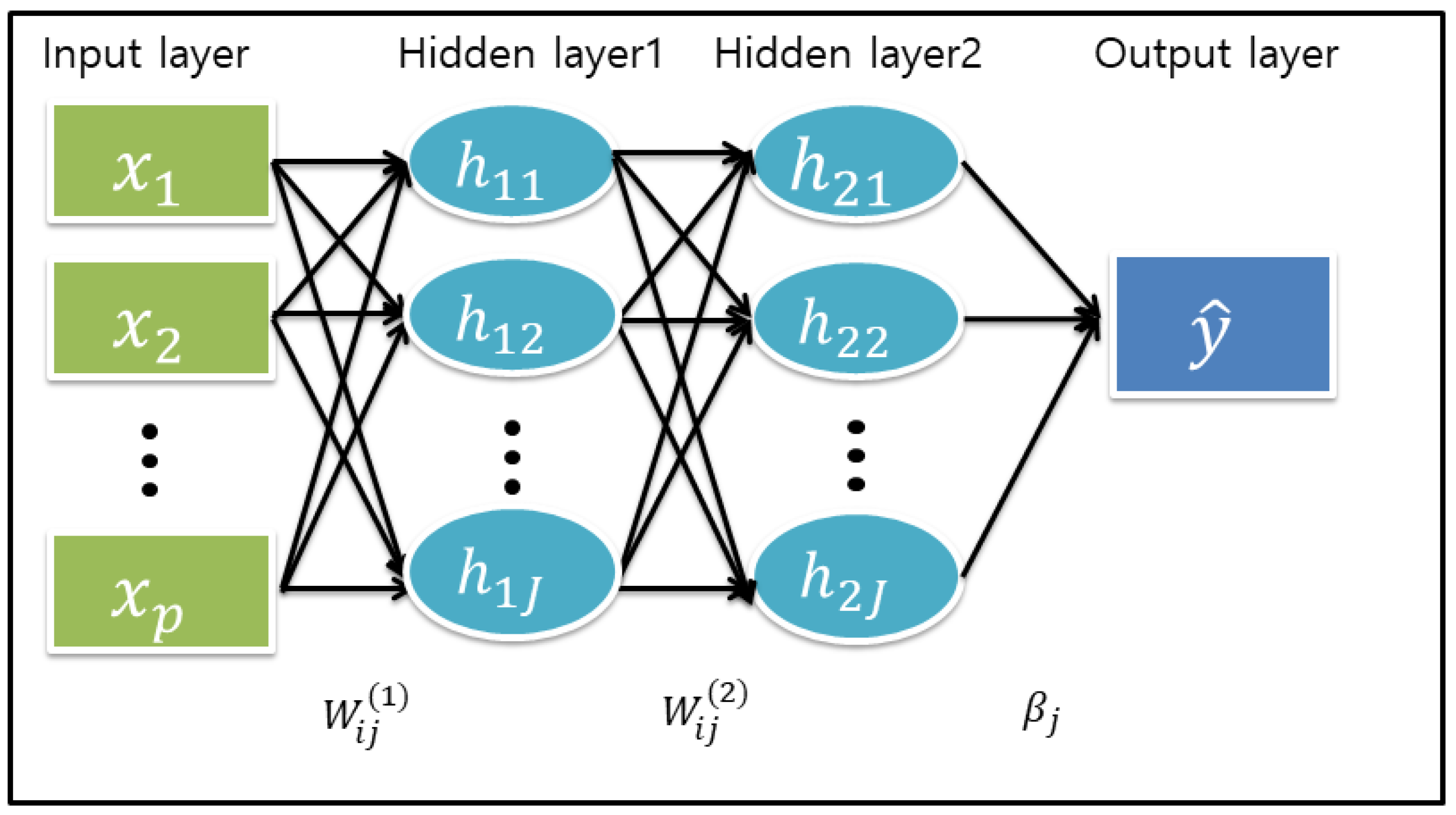
Below, we outline a framework of the DL model with a feed-forward neural network (FNN) architecture. We first describe an analytical form of the DL model. It consists of one input layer with p input nodes, L hidden layers with hidden nodes, and one output layer with K output nodes. For simplicity of argument, we consider the DL model with and . Then, the two hidden layers with p input variables ’s are given by the following forms [1]
and the output layer is
where and the jth node (unit) of thesecond (final) hidden layer depends on weights in the hidden layer and features in the input layer. Here, and values, including bias (intercept) terms and are input and output weights (unknown parameters), respectively, and , and are activation functions for the first, second and output layers. For a graphical representation of a simple DL model with a two-hidden layer of , see Figure 1. In fact, the FNN DL model above can be viewed as a recursive GLM [7] where the activation function corresponds to an inverse link function in the GLM. The activation function can be pre-specified as a nonlinear function (e.g., sigmoid, ReLU with max) in the hidden layer and as a linear or nonlinear function according to the type of response y in the output layer. For example, for the activation function of the output layer, we can use a linear function for continuous response data and an exponential function for count response data.

Figure 1.
A feed-forward deep learning model with two-hidden layers where bias terms are omitted for brevity but are written in the main text.
The DL model is fitted via the following learning algorithms during a training process. The unknown weights are estimated by minimizing the objective function (denoted by ) based on the empirical loss function (e.g., squared loss or negative log-likelihood) over all the training data. For example, for the squared loss, we have that
where is the ith component of in the output layer above. The computation of for minimizing can be implemented using backpropagation and a stochastic gradient descent (SGD) optimization method such as the Adam algorithm [24]. It can be crucial to appropriately choose or tune the hyper-parameters (e.g., the depth (L) and width ()) due to their sensitivity to the performance of the DL model. For more details, see [1,3]. The initial idea of the NN is a brain chain reaction neurons’ network, and the applications of NN can be found in [2,25,26,27,28,29]. Hereafter, we call the DL and NN models using Kim and Ha’s method [16] to be DL and NN models, respectively. For data analysis for the DL and NN models, we used the ’neuralnet’ R package [30] training neural networks using backpropagation and logistic activation function for smoothing the result of the cross product of the covariate or neurons and the weights by using the ’neuralnet’ command. We also followed the procedures of Kim and Ha’s DL and NN methods for count response [16]. First, we normalize the whole data including count output variable and input variables with the normalizing formula:
and we divide 80% normalized training data and 20% normalized test data from the standardized whole data. Second, we fit the normalized training data to either the DL or NN regression models in order to find the best model. Third, we apply the normalized test data to the best model of DL or NN based on the normalized train data. Fourth, we find the predicted values from the model. Fifth, we transform the normalized predicted values back to the original data format as follows
and we calculate the residual with the transformed predicted values and original count test data. Lastly, we perform the above procedures 1000 times to produce the root mean square error (RMSE) to determine the accuracy of each model.
3. Simulation Study
3.1. Simulation Setup
We generate highly correlated normal and non-normal simulated data to compare the methods we mentioned in the previous session. For non-normal simulated data, we used a copula function in this paper. Copulas are a good statistical method for finding multivariate dependence structures because copulas do not require normality, linearity, or independence assumptions. See [31,32] for detailed information about copulas. To construct a highly correlated dependence structure of input variables, we employ the Archimedean Clayton copula function. The reason that we choose the Clayton copula function for the simulation study is that the Clayton copula function has lower tail dependence. The insurance data have more lower tail dependence rather than upper tail dependence because most claims are either zero or one. In the simulation study, we considered two cases. The first case is a multivariate normal distribution simulation data, and the second case is the non-normal simulated combined data consisting of multivariate normal data, binary data, and copula-based simulated data. The first simulation setup is that twelve input variables are generated from the multivariate normal distribution with mean and covariance matrix A as follows:
The output variable was randomly generated from a uniform distribution from 0 to 10. The values of the response variable are 0 to 10 integers. The number of observations for each output and input variable is 1000.
The second simulation setup takes as input variables. The first four variables are generated from the multivariate normal distribution with mean and covariance matrix:
The next thirty variables are generated by the Clayton copula function, and the last six variables are binary variables (0 or 1). We set up the parameters for the Clayton copula function with a dependence parameter equaling to 8 and the number of dimensions equaling to 30. We generated a random sample of 1000 observations from the copula. The random sample is assigned to the input variables. The input variables generated by copula function follow the uniform distribution (0,1) so that all values are in between the range of 0 and 1. We then multiply 10 to all input variables and then rounded the decimal values to integers. To help readers understand the detailed simulation setup better, we included R codes in Appendix A. To employ PCA-based GLM in this paper, we used five principal components which can explain enough of the total variation of our data by using R commands (see Appendix A). Readers can change the number of principal components depending on how many highly correlated covariates they have in order to explain the total variation of data. We also include a GBM method for comparison. We uses R package “gbm” in this paper. To understand the GBM method, we recommend reading [33]’s tutorial for gradient boosting machines. In our paper, we used the R commands (see Appendix A). To compare the accuracy of the DL, NN, DLk, GBM, and PCA-based POI, NB and ZIP models [14,15], each using the simulated data displayed in Table 1, we employ the root mean square error (RMSE) formula as follows:
where RMSE = root mean squared error, , the number of observations, the actual observation, and the predicted value of the observation.

Table 1.
RMSE of Simulated Multivariate Normal Data and Non-Normal Combined Data with Multivariate Normal, Copula and Binary Data under 1000 Repetitions.
For the multivariate normal simulated data and non-normal simulated data combined with the multivariate normal, Clayton copula, and binary data, we randomly generate input and output data with a sample size of 1000. We then take a random sample of 800 observations (training data) from the generated data 1000 observations with 1000 repetitions. We compute the RMSEs with the predicted values from the DL, NN, DLk, GBM, POI, NB and ZIP models and 20% testing data for the three simulated cases in Table 1. The DL model was built with double hidden layers with (2,2) neurons, and the NN model was built with a single hidden layer with two neurons for each multivariate normal, Clayton copula and binary combined case. For the simulation study of the DLk model, we followed Kim and Ha’s basic settings including the transformed normalization of the input and output variables; we also set two hidden layers with two neurons in each hidden layer, sigmoid activation functions in each layer dense command in Keras, and mean squared error loss.
3.2. Simulation Results
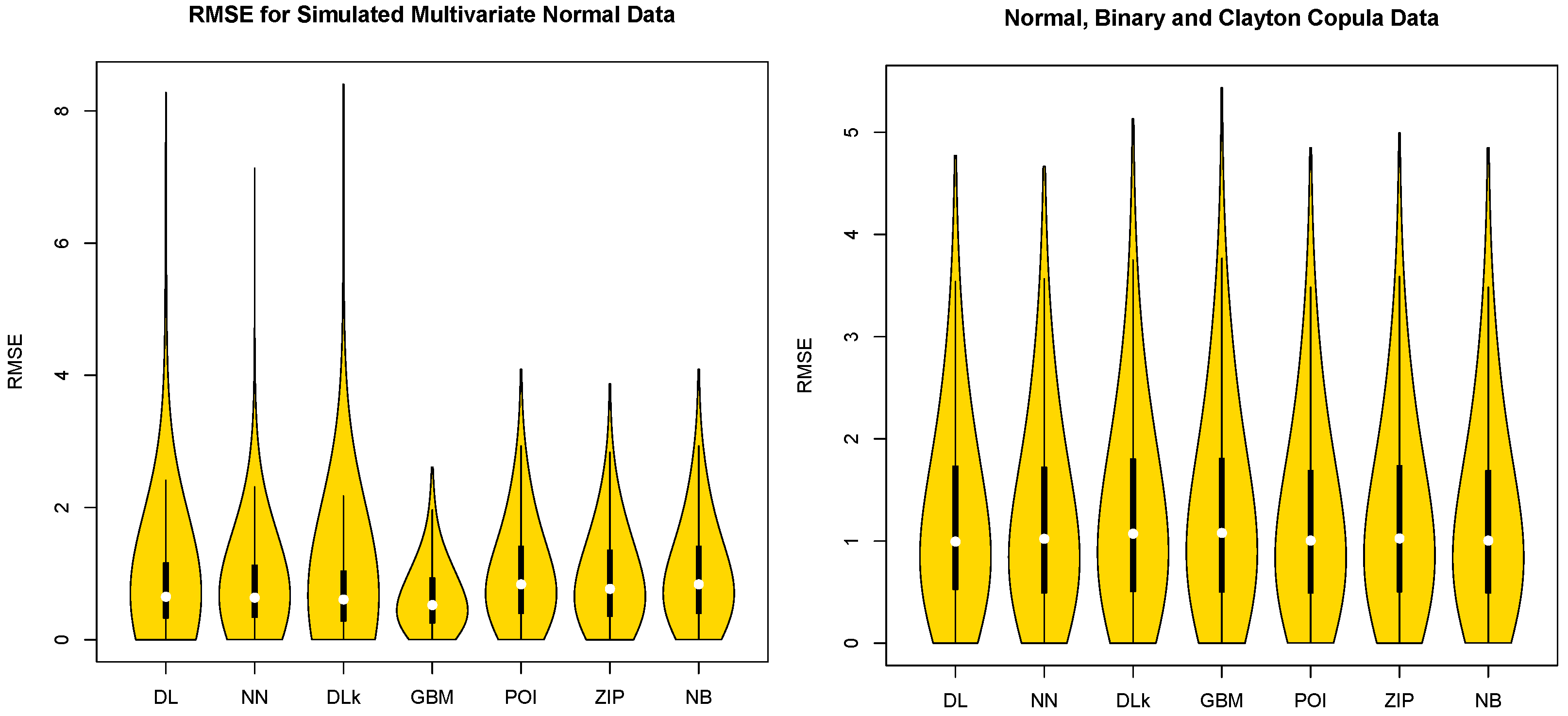
Table 1 shows that the GBM model is the best model for the multivariate normal distribution simulation case in terms of the median and IQR for RMSE and that the DL model is the best model for the combined non-normal simulated case with multivariate normal distribution, Clayton copula, and binary data in terms of the median for RMSE. Table 1 also shows that the NN model has the smallest maximum value of RMSE for the combined non-normal simulated data. These findings coincide with the results from [11,12] in that the DL and NN models for binary response data are more efficient than the PCAGLM with logit and PCA-GLM with probit models. The Violin plots in Figure 2 confirm that the GBM model for the multivariate normal distribution simulation case is superior to the DL, NN, DLk, POI, ZIP, and NB models in terms of the median and IQR, and the DL model for each non-normal combined simulation case with multivariate normal, Clayton copula and binary shows a superiority over the NN, DLk, GBM, POI, ZIP and NB models in terms of the median.
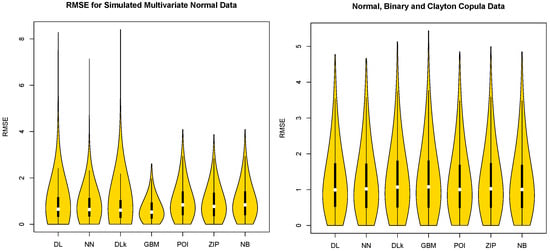
Figure 2.
Violin Plots of RMSE with Simulated Multivariate Normal Data and Non-Normal Combined Data with Multivariate Normal, Copula and Binary Data.
4. Illustrated Data Analysis
To compare the accuracy of DL, NN, DLk, GBM, PCA-based POI, NB and ZIP models with real insurance-related data, we used speeding ticket data from [34] and Singapore automobile claims data from the R Package insuranceData, which came from [35]. The speeding ticket dataset has 68,357 observations across nine variables. Table 2 contains descriptions of the nine variables that we used in our analysis. For our analysis, ’Amount’ was used as the output variable Y, and the remaining eight variables were used as the input variables.
Table 2.
Variables and description of speeding ticket data.
The Singapore automobile claims data were used for proposing hierarchical models of Singapore driving experience by [36]. The data can be downloaded from the general insurance association of Singapore organization website: www.gia.org.sg (accessed on 5 February 2022). The data features 7483 observations and 13 variables. Table 3 shows the variables in the Singapore automobile claims dataset that we used for our data analysis. Here, ’Clm Exp Count’ (number of claims during the year) was used as the output variable Y, and the remaining 12 variables were used as input variables.
Table 3.
Variables and description of Singapore automobile claims data.
For the two real datasets, we take a random sample of 800 observations from the real data observations with 1000 repetitions. We compute the RMSEs with the predicted values from the DL, NN, DLk, GBM, POI, NB, and ZIP models and 20% testing data for the two real data cases in Table 4. Table 4 shows that the DL model is the best model for the large size speeding ticket dataset in terms of the median for RMSE and that the NN model is the best model for the smaller size Singapore auto claims dataset in terms of IQR. This may be because large real insurance-related datasets can follow a multivariate non-normal distribution. These results coincide with the result of the multivariate non-normal simulated case shown in the Table 1. Violin plots in Figure 3 confirm that the DL model has the smallest maximum value of RMSE and is superior to the NN, DLk, GBM, POI, ZIP, and NB models in terms of the median. The DL model was built with double hidden layers with (2,2) neurons, and the NN model was built with a single hidden layer with two neurons for each real datum. For the real data analysis with the DLk model, we set the same settings as the DL and NN, with double hidden layers with (2,2) neurons.
Table 4.
RMSE of speeding ticket data and Singapore automobile claims with 1000 repetitions.
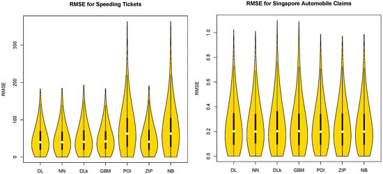
Figure 3.
Plots of RMSE with real data.
5. Conclusions
In this research, we compare Kim and Ha’s DL and NN models for the non-normal highly correlated input variables with DLk, GBM, PCA-based POI, ZIP, and NB models in terms of accuracy using the median of RMSE. With simulated non-normal data and real insurance-related data, we showed that the DL model is superior to the NN, DLk, GBM, POI, ZIP, and NB models in terms of the median. With simulated normal data, we showed that the GBM model is superior to the DL, NN, DLk, POI, ZIP and NB models in terms of the median and IQR. In terms of computation time, Kim and Ha’s DL and NN models are much faster than the DLk model. When we deal with a large insurance claim non-normal data, the Kim and Ha’s DL model can be a fast and accurate prediction model. In future studies, we will consider bivariate or multivariate count response variables allowing for highly correlated non-normal input variables with Kim and Ha’s DL and NN models. We will also consider insurance description text count data analysis with the textual data mining method and Kim and Ha’s DL and NN models.
Author Contributions
Conceptualization, J.-M.K. and I.D.H.; methodology, J.-M.K. and I.D.H.; software, J.-M.K. and J.K.; validation, J.-M.K., J.K. and I.D.H.; formal analysis, J.-M.K. and J.K.; investigation, J.-M.K. and I.D.H.; resources, I.D.H.; data curation, J.-M.K. and I.D.H.; writing—original draft preparation, J.-M.K. and I.D.H.; writing—review and editing, I.D.H.; visualization, J.-M.K. and J.K.; supervision, I.D.H.; project administration, J.-M.K. and I.D.H.; funding acquisition, I.D.H. All authors have read and agreed to the published version of the manuscript.
Funding
National Research Foundation of Korea (NRF) funded by the Ministry of Education (No. NRF-2020R1F1A1A01056987).
Institutional Review Board Statement
Not applicable.
Informed Consent Statement
Not applicable.
Data Availability Statement
Not applicable.
Conflicts of Interest
The authors declare no conflict of interest.
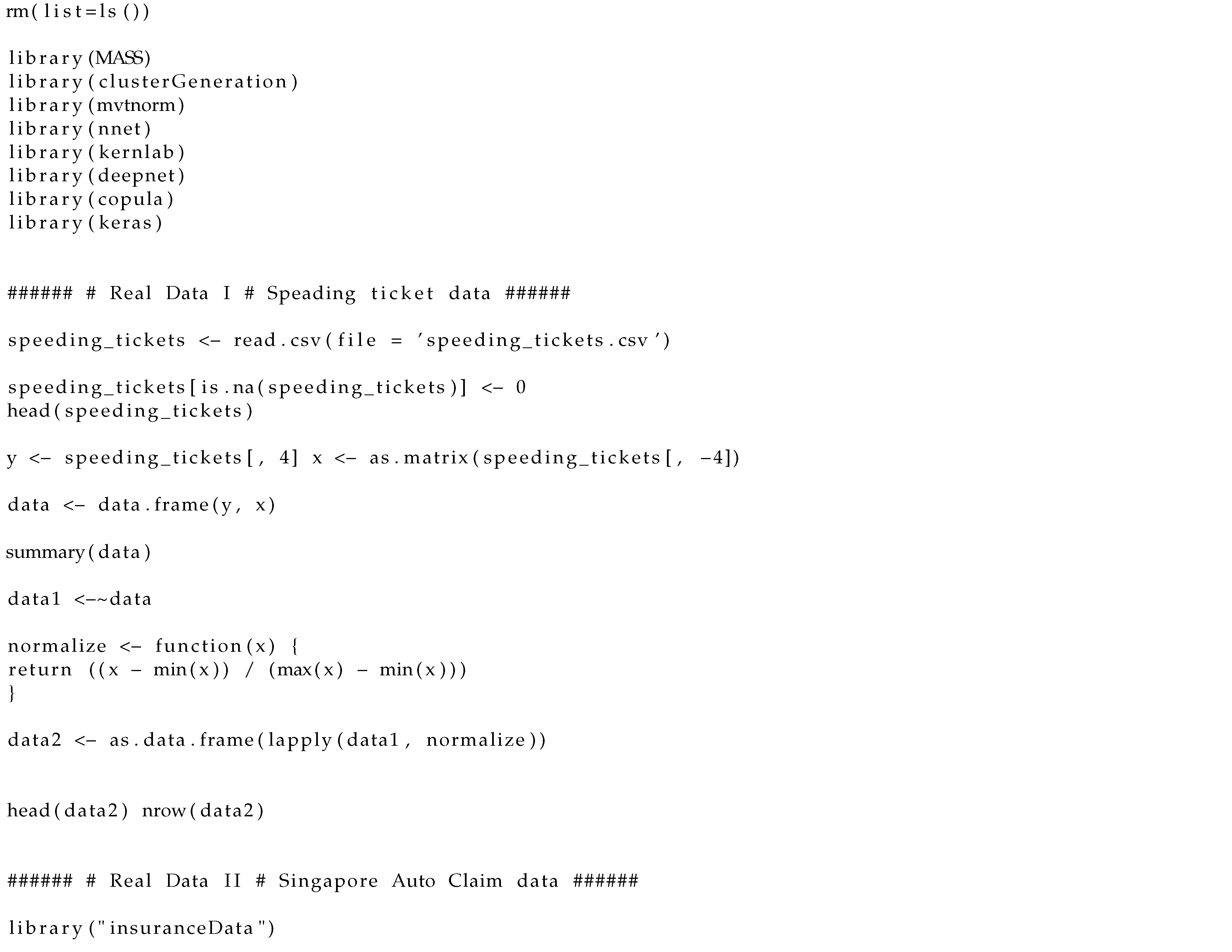
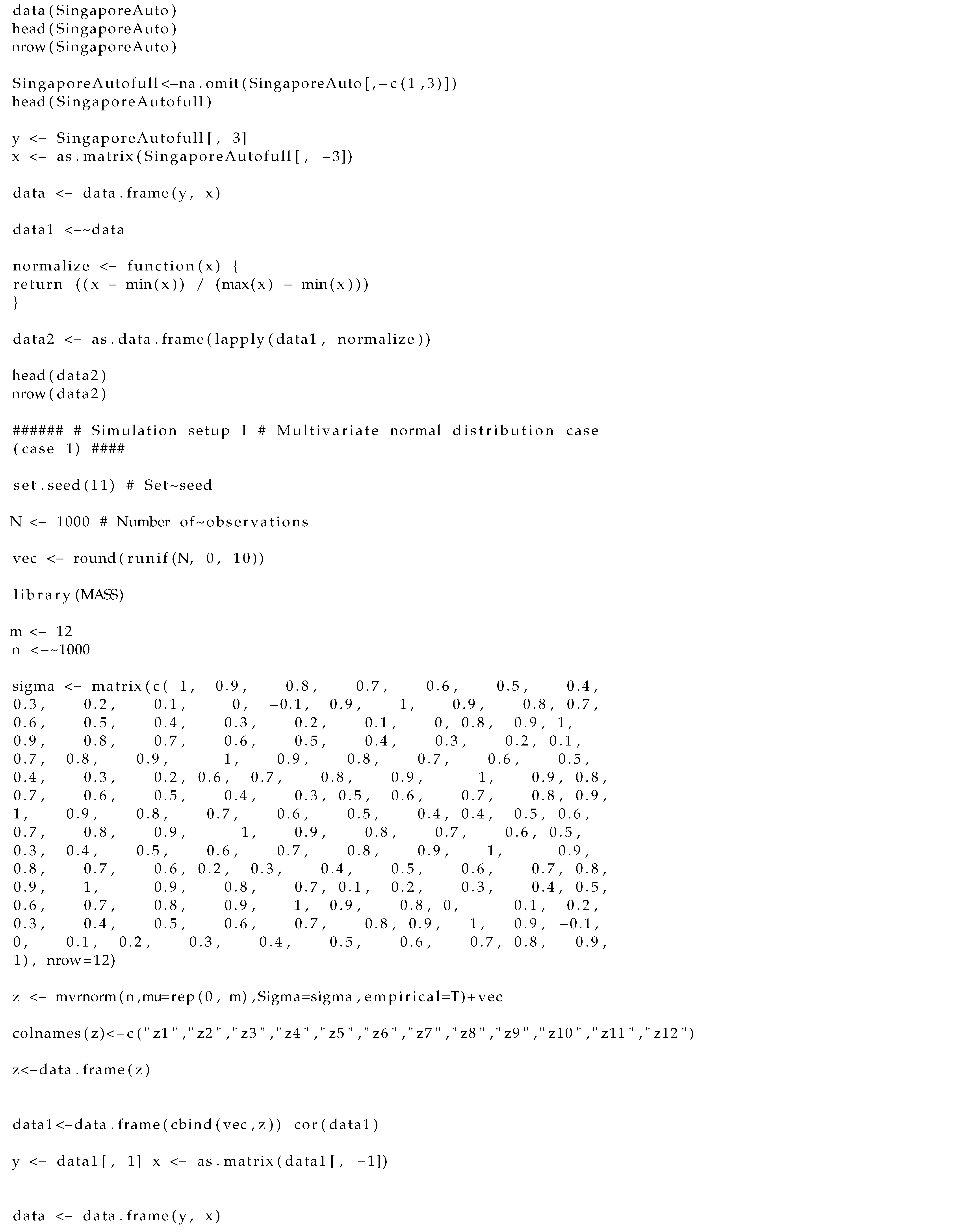
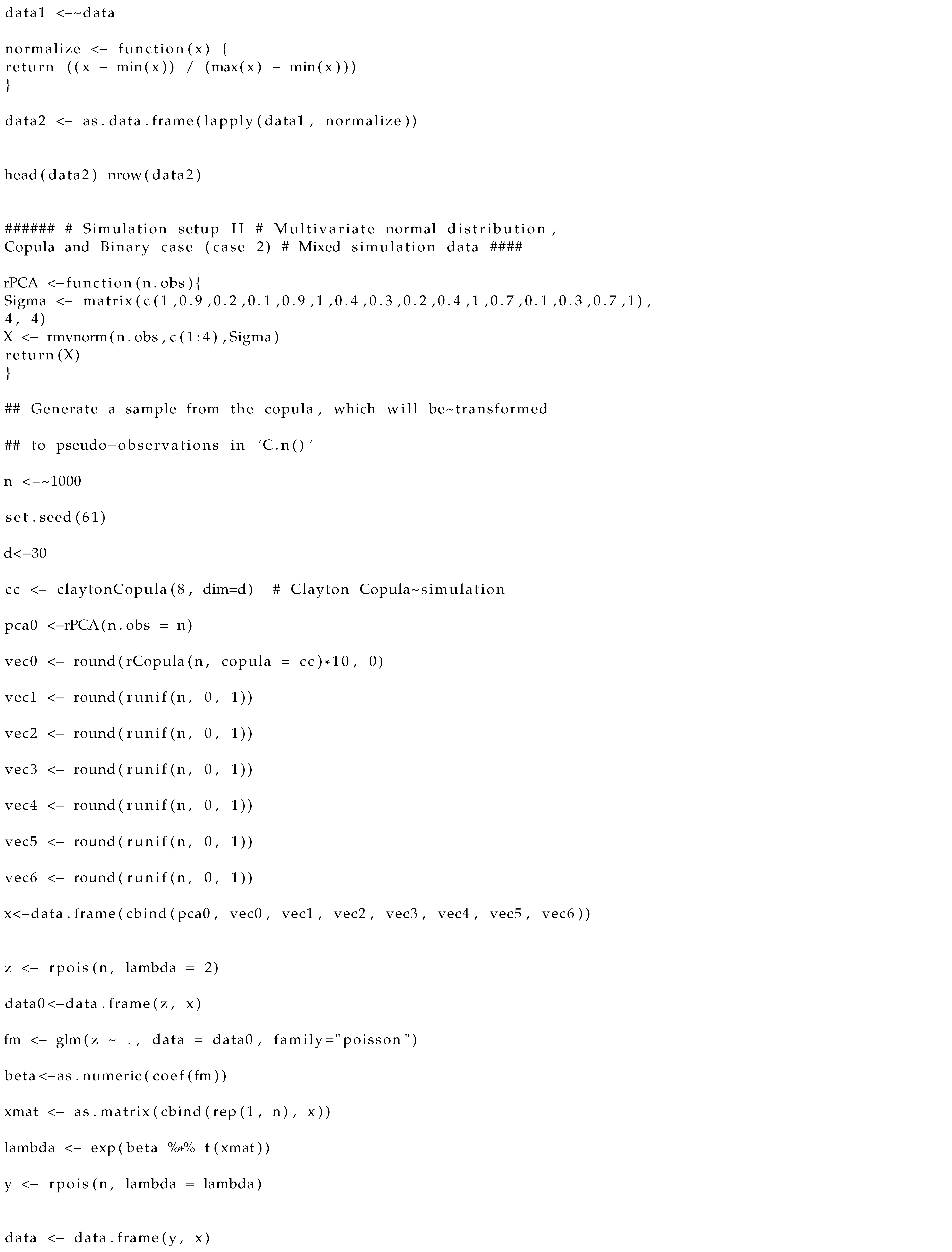
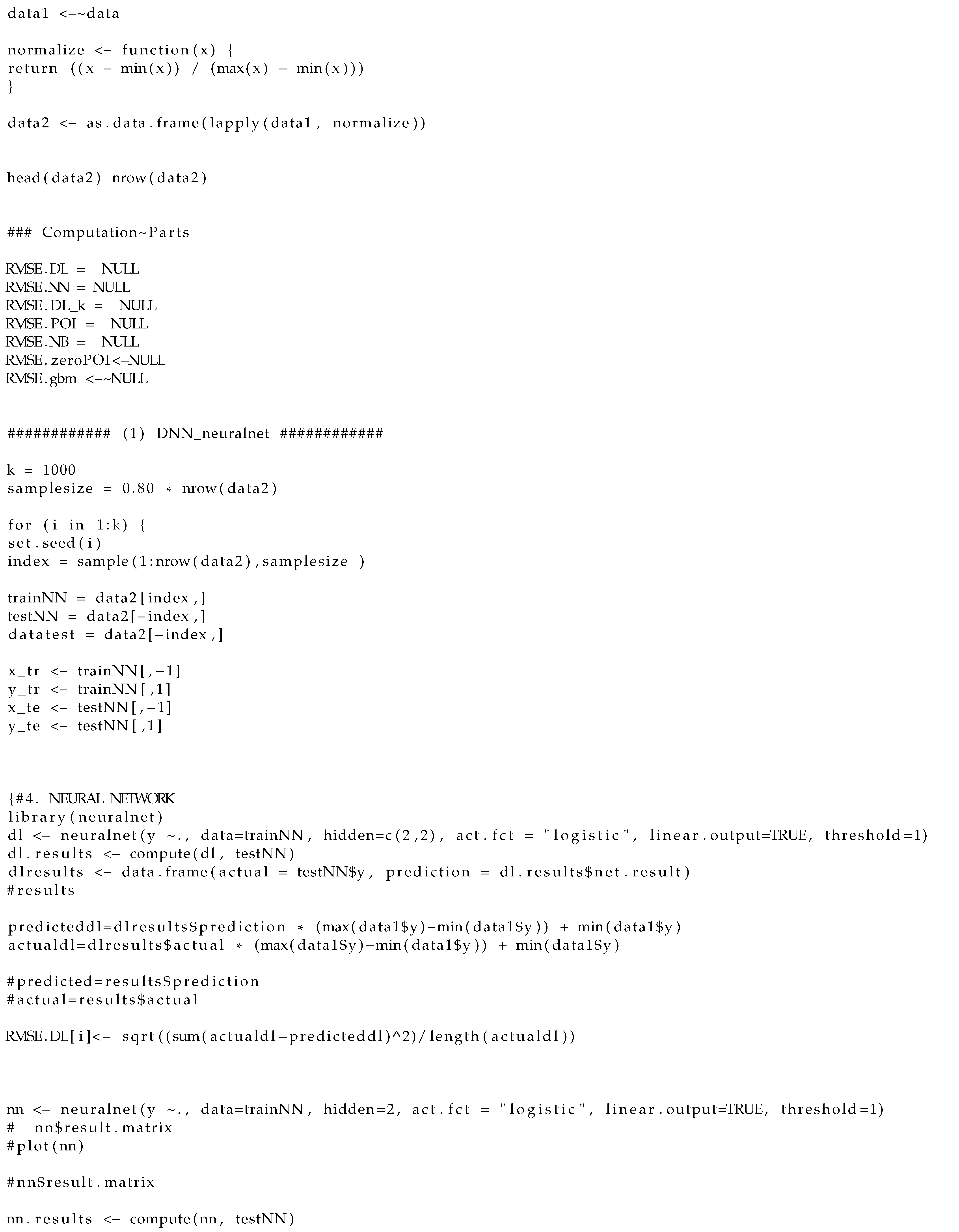
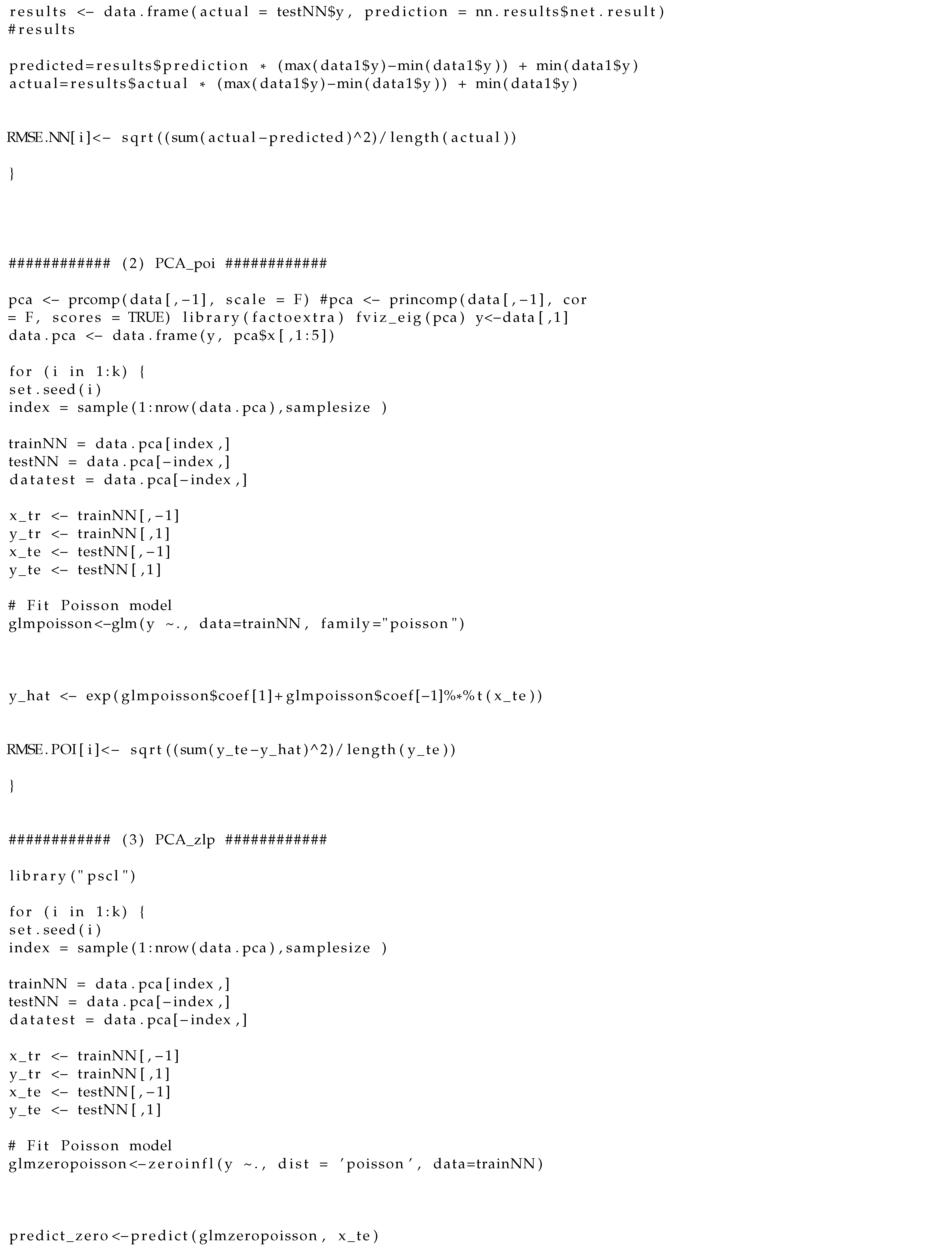
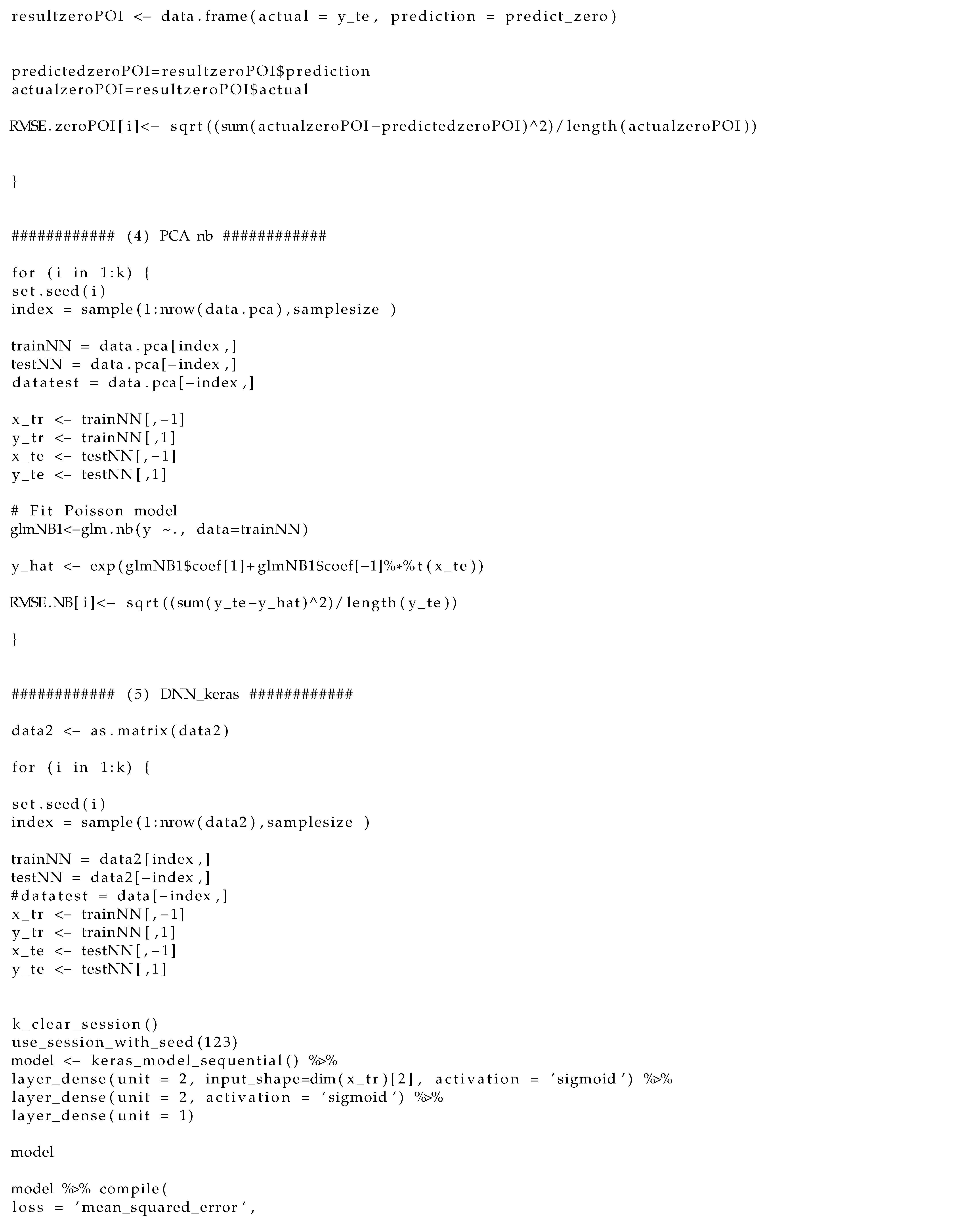
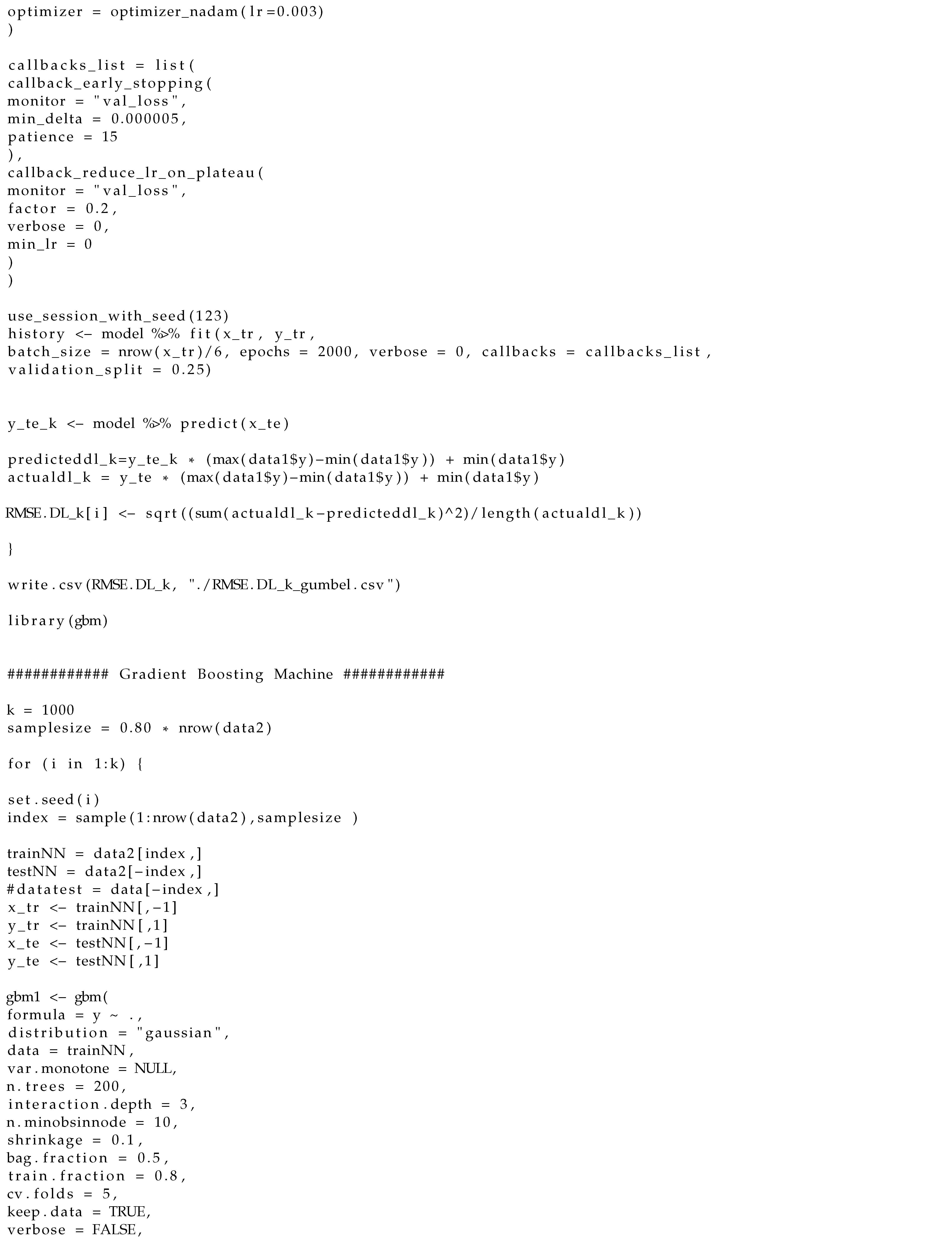
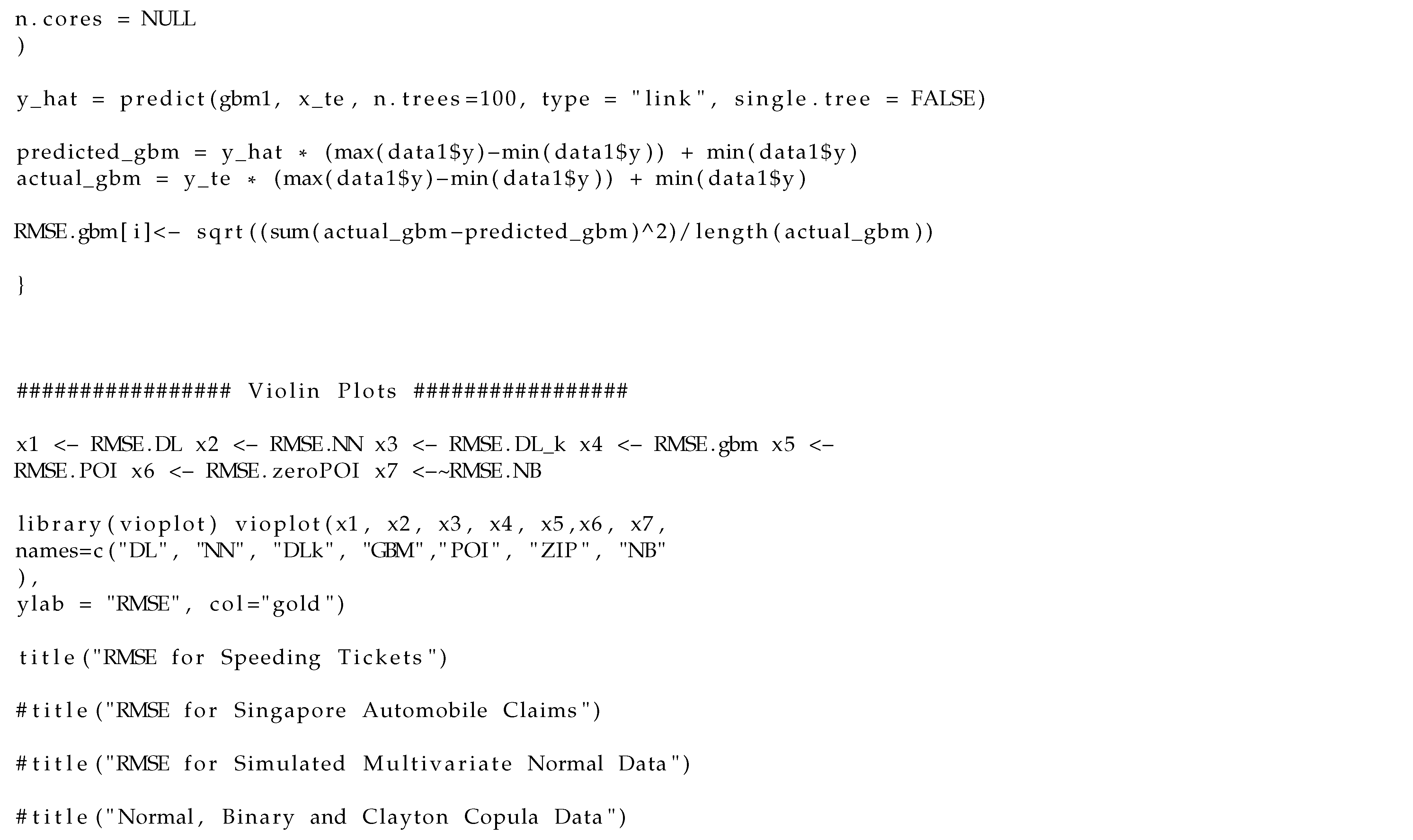
Appendix A. R Codes for Data Analysis
The following R codes produce the results of our real data analysis.
References
- Goodfellow, I.; Bengio, Y.; Courville, A. Deep Learning; MIT Press: Cambridge, MA, USA, 2016. [Google Scholar]
- LeCun, Y.; Bengio, Y.; Hinton, G. Deep learning. Nature 2015, 521, 436–444. [Google Scholar] [CrossRef] [PubMed]
- Fan, J.; Ma, C.; Zhong, Y. A selective overview of deep learning. Stat. Sci. 2021, 36, 264–290. [Google Scholar] [CrossRef] [PubMed]
- Farrell, M.H.; Liang, T.; Misra, S. Deep neural networks for estimation and inference. Econometrica 2021, 89, 181–213. [Google Scholar] [CrossRef]
- Sun, T.; Wei, Y.; Chen, W.; Ding, Y. Genome-wide association study-based deep learning for survival prediction. Stat. Med. 2020, 39, 4605–4620. [Google Scholar] [CrossRef] [PubMed]
- Montesinos-Lopez, O.A.; Montesinos-Lopez, J.C.; Salazar, E.; Barron, J.A.; Montesinos-Lopez, A.; Buenrostro-Marisca, l.R.; Crossa, J. Application of a Poisson deep neural network model for the prediction of count data in genome-based prediction. Plant Genome 2021, 14, e20118. [Google Scholar] [CrossRef]
- Polson, N.G.; Sokolov, V. Deep learning: A Bayesian perspective. Bayesian Anal. 2017, 12, 1275–1304. [Google Scholar] [CrossRef]
- Tran, M.-N.; Nguyen, N.; Nott, D.; Kohn, R. Bayesian deep net GLM and GLMM. J. Comput. Graph. Stat. 2020, 29, 97–113. [Google Scholar] [CrossRef]
- Rai, R.; Tiwari, M.K.; Ivanov, D.; Dolgui, A. Machine learning in manufacturing and industry 4.0 applications. Int. Prod. Res. 2021, 59, 4773–4778. [Google Scholar] [CrossRef]
- Kim, J.-M.; Liu, Y.; Wang, N. Multi-stage change point detection with copula conditional distribution with PCA and functional PCA. Mathematics 2020, 8, 1777. [Google Scholar] [CrossRef]
- Kim, J.-M.; Wang, N.; Liu, Y.; Park, K. Residual Control Chart for Binary Response with Multicollinearity Covariates by Neural Network Model. Symmetry 2020, 12, 381. [Google Scholar] [CrossRef] [Green Version]
- Kim, J.-M.; Ha, I.D. Deep Learning-Based Residual Control Chart for Binary Response. Symmetry 2021, 13, 1389. [Google Scholar] [CrossRef]
- Skinner, K.R.; Montgomery, D.C.; Runger, G.C. Process monitoring for multiple count data using generalized linear model-based control charts. Int. J. Prod. Res. 2003, 41, 1167–1180. [Google Scholar] [CrossRef]
- Park, K.; Kim, J.-M.; Jung, D. GLM-based statistical control r-charts for dispersed count data with multicollinearity between input variables. Qual. Reliab. Eng. Int. 2018, 34, 1103–1109. [Google Scholar] [CrossRef]
- Park, K.; Kim, J.-M.; Jung, D. Control Charts Based on Randomized Quantile Residuals. Appl. Stoch. Model. Bus. Ind. 2020, 36, 716–729. [Google Scholar] [CrossRef]
- Kim, J.M.; Ha, I.D. Deep Learning-Based Residual Control Chart for Count Data. Qual. Eng. 2022, 34. [Google Scholar] [CrossRef]
- Sakthivel, K.M.; Rajitha, C.S. A Comparative Study of Zero-inflated, Hurdle Models with Artificial Neural Network in Claim Count Modeling. Int. J. Stat. Syst. 2017, 12, 265–276. [Google Scholar]
- Sakthivel, K.M.; Rajitha, C.S. Artificial Intelligence for Estimation of Future Claim Frequency in Non-Life Insurance. Glob. J. Pure Appl. Math. 2017, 13, 1701–1710. [Google Scholar]
- Sakthivel, K.M.; Rajitha, C.S. Model selection for count data with excess number of zero counts. Am. J. Appl. Math. Stat. 2019, 7, 43–51. [Google Scholar] [CrossRef]
- Goundar, S.; Prakash, S.; Sadal, P.; Bhardwaj, A. Health Insurance Claim Prediction Using Artificial Neural Networks. Int. J. Syst. Dyn. Appl. 2020, 9, 40–56. [Google Scholar] [CrossRef]
- Haghani, S.; Sedehi, M.; Kheiri, S. Artificial neural network to modeling zero-inflated count data: Application to predicting number of return to blood donation. J. Res. Health Sci. 2017, 17, 1–4. [Google Scholar]
- Rodrigo, H.; Tsokos, C. Bayesian modelling of nonlinear Poisson regression with artificial neural networks. J. Appl. Stat. 2020, 47, 757–774. [Google Scholar] [CrossRef]
- McCullagh, P.; Nelder, J.A. Generalized Linear Models; Chapman and Hall: New York, NY, USA, 1989. [Google Scholar]
- Kingma, D.P.; Ba, J. Adam: A method for stochastic optimization. arXiv 2014, arXiv:1412.6980. [Google Scholar]
- Agatonovic-Kustrin, S.; Beresford, R. Basic concepts of artificial neural network (ANN) modeling and its application in pharmaceutical research. J. Pharm. Biomed. Anal. 2000, 22, 717–727. [Google Scholar] [CrossRef]
- Hassabis, D.; Kumaran, D.; Summerfield, C.; Botvinick, M. Neuroscience-inspired artificial intelligence. Neuron 2017, 95, 245–258. [Google Scholar] [CrossRef] [PubMed] [Green Version]
- Masood, I.; Hassan, A. Pattern Recognition for Bivariate Process Mean Shifts Using Feature-Based Artificial Neural Network. Int. J. Adv. Manuf. Technol. 2013, 66, 1201–1218. [Google Scholar] [CrossRef] [Green Version]
- Addeh, A.; Khormali, A.; Golilarz, N.A. Control Chart Pattern Recognition Using RBF Neural Network with New Training Algorithm and Practical Features. ISA Trans. 2018, 79, 202–216. [Google Scholar] [CrossRef]
- Zan, T.; Liu, Z.; Su, Z.; Wang, M.; Gao, X.; Chen, D. Statistical Process Control with Intelligence Based on the Deep Learning Model. Appl. Sci. 2020, 10, 308. [Google Scholar] [CrossRef] [Green Version]
- Fritsch, S.; Günther, F.; Wright, M.N.; Suling, M.; Mueller, S.M. Training of Neural Networks; R Package, neuralnet; R Foundation for Statistical Computing: Vienna, Austria, 2019. [Google Scholar]
- Nelsen, R.B. An Introduction to Copulas, 2nd ed.; Springer: New York, NY, USA, 2006. [Google Scholar]
- Kim, J.-M. A Review of Copula Methods for Measuring Uncertainty in Finance and Economics. Quant. Bio-Sci. 2020, 39, 81–90. [Google Scholar]
- Alexey, N.; Alois, K. Gradient boosting machines, a tutorial. Front. Neurorobotics 2013, 7, 21. [Google Scholar] [CrossRef] [Green Version]
- Makowsky, M.D.; Stratmann, T. Political Economy at Any Speed: What Determines Traffic Citations? Am. Econ. 2009, 99, 509–527. [Google Scholar] [CrossRef]
- Wolny-Dominiak, A.; Trzesiok, M. A Collection of Insurance Datasets Useful in Risk Classification in Non-life Insurance; R Package, insuranceData; R Foundation for Statistical Computing: Vienna, Austria, 2014. [Google Scholar]
- Frees, E.W.; Valdez, E.A. Hierarchical Insurance Claims Modeling. J. Am. Stat. 2008, 103, 1457–1469. [Google Scholar] [CrossRef] [Green Version]

Publisher’s Note: MDPI stays neutral with regard to jurisdictional claims in published maps and institutional affiliations. |
© 2022 by the authors. Licensee MDPI, Basel, Switzerland. This article is an open access article distributed under the terms and conditions of the Creative Commons Attribution (CC BY) license (https://creativecommons.org/licenses/by/4.0/).