A Simple Greedy Heuristic for Site Specific Management Zone Problem

Abstract

In agriculture, the soil properties influence the productivity and quality of crops. The farmer expects that in a specific area of the land, the physicochemical characteristics of the soil will be homogeneous as the selected crop has the desired quality and minimizes the use of fertilizers. There are three approaches to determining the correct delimitation of the land in the state-of-the art. The first one (k-means and fuzzy k-means) is impractical for current agricultural technology. The second approach is based on integer linear programming and a pre-processing step. This approach limits the shapes of delimited zones to rectangular, and the third approach extends the solution search space and generates orthogonal regions using Estimation of Distribution Algorithms (EDA). In this work, we generate orthogonal regions with a different approach to the EDA, a greedy construction heuristic. Our heuristic produces feasible solutions with a reasonable running time compared with the running times of EDA.

1. Introduction

The applications of operations research are numerous and belong to a wide variety of fields of knowledge. One of these fields of knowledge is agriculture [1,2]. In particular, the part of agriculture that deals with crop planning to obtain crops with specific physical and chemical characteristics is reflected in the products’ quality. This area is known as precision agriculture.

In [3], Ortega et al. proposed the following problem. A farmer who wants to know how much fertilizer he should use in one of his crops takes a sample of the crop soil area of interest. Depending on the levels of nutrients detected in the sample, an amount of fertilizer will be necessary. However, it is a fact that farmland does not have uniform soil properties, so it is necessary to take different samples to deal with this variability of soil properties.

The Site Specific Management Zone (SSMZ) problem allows us to not have to make too many changes in the necessary fertilizer levels since a relative variance is considered between samples that belong to the same region. There is an indicator to measure this relative variance globally, and it is known as homogeneity. The farmers consider this parameter to know if the delimited regions have a slight variance concerning the samples that form them [3]. The delimited regions’ shape is directly designed to work with current and massively used agricultural technology (tractors).

The weather is a factor that can alter soil properties and affect subsequent crops. Suppose we want to consider how much the climate affects these properties over time. In that case, we think of a robust delimitation problem where the delimitation is simultaneously resistant to changes in all soil properties. This work is limited to specific measurements of soil properties and delimitation that consider the properties separately.

The SSMZ manages soil, pests, and crops based on the spatial variation within a field. Therefore, nutrient management plans for site-specific situations should minimize undesired environmental effects while optimizing whole-farm profits and production. The SSMZ comprises delimited areas according to specific physicochemical characteristics of the soil, so the planned crop optimally uses them. This decision about soil allows us to take advantage of the characteristics according to the crop. However, Corwin [4] points out that it is essential to consider the complex interactions between the following factors:

• Edaphic, such as salinity, nutrients;
• Biological, earthworms, microbes, etc;
• Anthropogenic, e.g., irrigation management, among others;
• Topographic, e.g., slope elevation;
• Meteorological, e.g., temperature, rainfall;
• How to divide the facility into regions,

where the facility is the land to be studied. In [5], Ortega and Santibáñez solved a case study related to corn crops using clustering techniques in an irregular-shaped facility based on a k-means proposed by the same authors in [6]; also in [7,8] solutions based on fuzzy k-means were proposed. The key problem with these k-means and fuzzy k-means is that they generate solutions with shapes that are difficult to process with current agricultural technology.

Next, in [9] Cid-Garcia et al. show a solution of SSMZ for rectangular facilities based on a delimitation of zones with rectangular area units as shown in Figure 1. In the same work, an integer linear program with a pre-processing step is proposed that generates feasible solutions with rectangular regions as in Figure 2. In this work, we assume that the facility shape is rectangular, and it is divided into rectangular area units. Finally, in [10], Velasco et al. introduce a metaheuristic approach based on Estimation of Distribution Algorithms (EDA) which is an extension of the rectangular-based solution in [9] due to their proposed orthogonal solutions to extend the quality and shape of the regions in a solution. In this work, we deal with that approach.

The criteria for the division of the facility depend on the proportion of some physicochemical properties in the soil like (pH, organic matter rate (OM), amount of phosphorus (P), and the sum of bases (SB). In this sense, each area unit is, simultaneously, a sample of soil with a numerical value associated to it. In [11,12], the authors show how to get this numerical value for each area unit. We assume this information is a part of the input of SSMZ. The objective of SSMZ is to minimize the number of regions of the facility under a homogeneity constraint. The homogeneity constraint is a global measure of the variation of specific properties of the soil and the number of regions of a facility.

2. Problem Statement

We define the Site Specific Management Zone (SSMZ) as follows:

Problem 1 

(SSMZ).

• Input: A facility M divided into $\left|M\right|$ of samples (area units) of the soil, a parameter $\alpha \in [0,1]$.
• Output: The facility divided into $Z=\{z_1,z_2,\dots z_k\}$ regions, with $\left|Z\right|$ minimum and $H\ge \alpha$.

$H\in [0,1]$ is the estimated homogeneity parameter and is defined in [5] as Equation (1).

$$H(M,Z)=1-\frac{{\sum }_{z\in Z}\left(\right|z|-1)·s^2\left(z\right)}{{\sigma }_T^2\left(\left|M\right|-\left|Z\right|\right),}$$

(1)

where $\left|M\right|$ is the number of area units in the facility, $\left|z\right|$ is the number of area units in the region z, $s^2\left(z\right)$ is the sampling variance of the region z, and ${\sigma }_T^2$ is the population variance of the facility. Equation (1) implies that the relative variance of the chosen regions is at least $\alpha$, which is a parameter (value given by the farmers) to guarantee a homogeneous behavior of the zoning method. Experts suggest that the best delineations of management zones are achieved with a desired homogeneity parameter $\alpha$ greater than 0.5.

3. Methodology

In this work, we proposed a greedy heuristic that needs the following definitions.

Definition 1.

A valid area unit is an area unit with indices in set $M=\left\{\right(i,j\left)\right|1\le i\le m,1\le j\le n\}$.

We built a graph $G_M=(V_M,E_M)$ where $V_M$ is the set of vertices such that each element of $V_M$ is associated with a valid area unit. We put an edge between two vertices if the associated area units share a side. In Figure 3, the vertices are shown as blue circles and the set of edges as red lines.

Definition 2.

A labeling of $V_M$ is a map $\ell :V_M\to Z$, where $Z\subset \mathbb{N}$ such that $\left|Z\right|=k$ is the set of labels (regions).

Definition 3.

A path over $G_M$ is a succession of non repeated vertices connected by edges of the set $E_M$.

Definition 4.

A monochromatic path is a path with the same label in all vertices of the path.

Definition 5.

Two vertices $u,v\in V_M$ with $\ell \left(u\right)=\ell \left(v\right)$ are path connected if there exists a monochromatic path over $G_M$ from u to v, as in Figure 4.

Definition 6.

A region $z\subseteq M$ is a set of valid area units where associated vertices have the same label.

Definition 7.

An orthogonal region is a region where all pairs of vertices on it are path connected or it is a region with a single associated vertex.

Definition 8.

A feasible labeling ℓ of $V_M$ is a labeling with only orthogonal regions.

Definition 9.

A feasible solution Z is a feasible labeling such that $H(M,Z)\ge \alpha$.

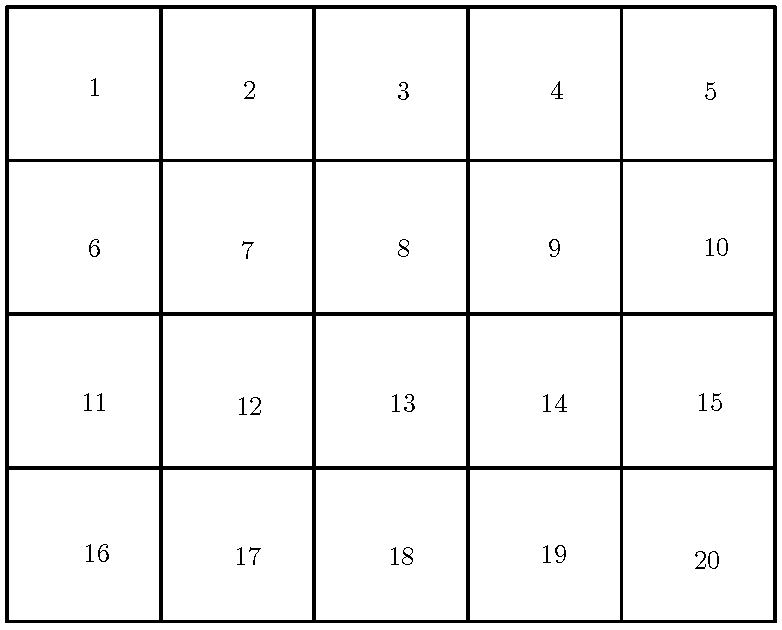
First, we propose an initial solution $Z_0$, where each vertex is a region with a single area unit, that is $\ell \left(u\right)\ne \ell \left(v\right)$ for all $u,v\in V_M$ with $u\ne v$, as with the blue labels in Figure 3. In [9] we can observe if $\alpha$ is near to 1, and if the number of regions needed to satisfy $H(V_M,Z_0)\ge \alpha$ is near to $|V_M|=mn$, therefore $Z_0$ is a feasible solution for SSMZ. To refer to each one of the area units of the facility, we will label them as shown in Figure 3.

Next, we try to merge adjacent area units, i.e., if two vertices $u,v\in V_M$ are connected by an edge and have a different label. We try to change the labels such that $\ell \left(u\right)=\ell \left(v\right)$. For a vertex $(i,j)$ we have up to four potential neighbors to merge with vertex $(i,j)$ as in Figure 5. It is easy to see that this merging step produces solutions with only orthogonal regions. Here, we do not directly consider the neighbors marked with red in Figure 5, because they can produce regions with path-disconnected vertices. There are two ways to avoid the generation of solutions with disconnected regions

• Only consider the neighbors $N_1(i,j)=\{(i-1,j),(i+1,j),(i,j-1),(i,j+1)\}$ to merge with an area unit $(i,j)$;
• We can consider the set of neighbors $N_2(i,j)$ to merge with an area unit $(i,j)$.

The elements of $N_2(i,j)$ depend on the elements of $N_1$. The activation of the elements of $N_2$ follows the next procedure and it is visualized in Figure 6.

• If a valid area unit $(i-1,j)$ is merged with $(i,j)$, then area units $(i-1,j-1)$ and $(i-1,j+1)$ are added to $N_2$ if they are valid.
• If a valid area unit $(i,j+1)$ is merged with $(i,j)$, then area units $(i-1,j+1)$ and $(i+1,j+1)$ are added to $N_2$ if they are valid.
• If a valid area unit $(i+1,j)$ is merged with $(i,j)$, then area units $(i+1,j-1)$ and $(i+1,j+1)$ are added to $N_2$ if they are valid.
• If a valid area unit $(i,j-1)$ is merged with $(i,j)$, then area units $(i-1,j-1)$ and $(i+1,j-1)$ are added to $N_2$ if they are valid.

It can be clearly seen that considering $N=(N_1\cup N_2)$ as a neighbor avoids solutions with disconnected regions because this construction allows only orthogonal regions. The criterion for deciding whether an area unit of N is merged with the area unit $(i,j)$ is that if a potential neighbor has merged, the value of H remains greater than or equal to the value of the parameter $\alpha$. The vertices whose label was changed in this step are marked so that their labels cannot be altered in the next merging steps. If this step is not included, there is a risk of generating an infeasible labeling.

After the merging step, the area unit $(i,j)$ must be marked as visited and added to the visited set (V). The new $(i,j)$ becomes an element of set $N\backslash V$; if set $N=\varnothing$ then the new $(i,j)$ is the pair $(i^{\prime },j^{\prime })$ with the smallest values for $i^{\prime }$ and $j^{\prime }$ and marked as not visited. Repeat until $V=M$. The whole procedure is shown in Algorithm 1.

Procedure $initializate\left(M\right)$ generates an initial solution where each area unit corresponds to a region and $|Z_0|=|M|$. Procedure $get{N}_1(i,j)$ gets the set $N_1$ of area unit $(i,j)$, similar to $get{N}_2(i,j)$. Procedure $merge$ relabels the area units. After the merge step in the move step, there are three ways to perform this procedure, as follows:

• $A_1$: New $(i,j)$ is the first nonvisited neighbor in lexicographical order from N;
• $A_2$: New $(i,j)$ is a random nonvisited neighbor from N;
• $A_3$: New $(i,j)$ is a nonvisited neighbor that produces a minimal decrease in H from N.

Note that the optimization process is implicit because we do not have an explicit objective function in Algorithm 1. However, it is implicit because the heuristic tries to generate fewer regions by mixing the existing ones. We must also remark that the search space in our method is bigger than the search space of the integer linear program. The above is because the shapes of the regions in our method are a super set of the set of shapes available in the integer linear program.

Algorithm 1 A simple greedy heuristic for the SSMZ problem.

Require:  A rectangle shape facility M divided in $m\times n$ area units, each one with a soil sample value. Ensure:  A feasible partition of facility M divided in Z regions. 1: $V\leftarrow \varnothing$ 2: $Z_0\leftarrow initialize\left(V_M\right)$ 3: $i\leftarrow 1$, $j\leftarrow 1$ 4: while$\left|V\right|<|V_M|$do 5:    $N_1\leftarrow ge{t}_{N_1}(i,j)$ 6:    $Z_0\leftarrow merge(Z_0,N_1)$ 7:    $N_2\leftarrow ge{t}_{N_2}(i,j,N_1)$ 8:    $Z_0\leftarrow merge(Z_0,N_2)$ 9:    $V\leftarrow V\cup \left\{\right(i,j\left)\right\}$ 10:    $[i,j]\leftarrow move(i,j,(N_1\cup N_2)\setminus V)$ 11: end whilereturn$Z_0$ 12: return$Z_0$

4. Experimental Results

The computational experiments were carried out on a personal computer with an AMD FX-8800P Radeon R7, Four-Core Processor @3.40 GHz, running the Linux operating system with Ubuntu 20.04 LTS, and 16 GB of RAM. The simple greedy heuristic was implemented in Python 3.8. For each facility size, there are ten instances where the fundamental difference is in the variance of sample soils of area units. For each instance, the homogeneity parameter $\alpha$ takes the values $\{0.5,0.7,0.9\}$, giving us 150 artificial instances and 40 real data instances, totaling 190 instances.

To evaluate the performance of the heuristic, we run 190 instances each with each algorithm variant. We calculate the percentage of each class of instances where our methods are better than or equal to the solutions provided using the MILP and EDA methods. In

Table 1. The percentages of instances of each class where the results of the proposed methods were better than or equal to the results of MILP and EDA methods.

Instance	${\mathit{A}}_1$		${\mathit{A}}_2$		${\mathit{A}}_3$
	MILP	EDA	MILP	EDA	MILP	EDA
Class 1	93.33%	10.00%	96.67%	70.00%	90.00%	16.67%
Class 2	93.33%	3.33%	100.00%	30.00%	83.33%	6.67%
Class 3	96.67%	0.00%	100.00%	16.67%	100.00%	3.33%
Class 4	100.00%	0.00%	100.00%	0.00%	100.00%	0.00%
Class 5	100.00%	6.67%	100.00%	26.67%	100.00%	6.67%
OM	80.00%	10.00%	100.00%	20.00%	70.00%	10.00%
Ph	60.00%	30.00%	100.00%	70.00%	40.00%	10.00%
P	100.00%	100.00%	100.00%	100.00%	100.00%	100.00%
SB	70.00%	20.00%	90.00%	30.00%	50.00%	10.00%

, we can observe that our method has better results than the MILP method in most instances. In counterpart, the EDA method gives us better results in most instances.

We can observe the performance of our heuristics in each real and artificial instance in

Table 2. Results of real data instances.

Instance	Alpha	${\mathit{Z}}_{\mathbf{EDA}}$	Time (s)	${\mathit{Z}}_{\mathbf{MILP}}$	Time (s)	${\mathit{A}}_1$		${\mathit{A}}_2$				${\mathit{A}}_3$
						Z	Time (s)	Z	Time (s)	${\mathit{Z}}_{\mathit{m}}$	s	Z	Time (s)
OM	1	40	23.28	40	0.01	40	0.05	40	5.38	40.00	0.00	40	0.05
	0.9	17	22.33	20	0.03	19	0.06	18	6.34	19.53	1.09	19	0.07
	0.8	11	22.73	17	0.12	17	0.05	14	6.09	15.95	0.91	17	0.06
	0.7	9	22.94	14	0.15	12	0.06	10	5.91	11.40	0.90	11	0.06
	0.6	6	23.17	11	0.08	9	0.05	7	5.74	9.59	1.43	10	0.06
	0.5	5	23.26	9	0.07	7	0.05	5	5.22	7.58	0.99	9	0.05
	0.4	4	23.33	7	0.07	7	0.04	5	4.98	6.66	1.30	9	0.07
	0.3	2	23.43	6	0.07	7	0.04	4	4.92	5.48	0.82	6	0.06
	0.2	2	23.47	5	0.14	4	0.04	3	4.63	4.80	0.89	6	0.05
	0.1	2	23.63	3	0.06	4	0.03	3	4.16	3.76	0.77	5	0.05
Ph	1	19	22.30	24	0.01	19	0.06	19	6.83	19.00	0.00	19	0.07
	0.9	13	22.33	17	0.08	16	0.06	15	6.80	16.46	0.54	17	0.06
	0.8	8	23.15	10	0.10	10	0.06	9	5.42	10.60	0.79	10	0.06
	0.7	6	23.28	7	0.07	8	0.04	6	5.13	8.55	1.14	10	0.06
	0.6	5	23.39	5	0.08	5	0.04	5	5.25	6.61	1.09	6	0.04
	0.5	4	23.45	4	0.08	4	0.05	4	4.38	5.37	0.63	5	0.05
	0.4	3	23.52	4	0.08	5	0.05	3	4.25	4.76	0.73	5	0.05
	0.3	3	23.62	3	0.06	4	0.04	3	4.18	4.19	0.72	4	0.05
	0.2	2	23.60	3	0.14	3	0.04	3	4.09	3.61	0.58	3	0.04
	0.1	2	23.64	2	0.01	3	0.05	2	3.86	2.87	0.44	3	0.04
P	1	32	21.46	33	0.01	32	0.06	32	6.23	32.00	0.00	32	0.06
	0.9	7	23.28	9	0.13	6	0.04	5	4.63	5.69	0.81	7	0.04
	0.8	4	23.46	5	0.19	3	0.04	3	4.06	3.02	0.14	3	0.05
	0.7	3	23.54	3	0.01	2	0.03	2	3.70	2.00	0.00	2	0.05
	0.6	2	23.64	3	0.01	2	0.04	2	3.71	2.00	0.00	2	0.05
	0.5	2	23.67	3	0.01	2	0.05	2	3.71	2.00	0.00	2	0.04
	0.4	2	23.67	3	0.01	2	0.04	2	3.84	2.02	0.14	2	0.04
	0.3	2	23.66	3	0.01	2	0.05	2	3.84	2.18	0.39	2	0.04
	0.2	2	23.64	3	0.08	2	0.04	2	3.94	2.17	0.38	2	0.04
	0.1	2	23.61	2	0.01	2	0.04	2	3.98	2.11	0.31	2	0.03
SB	1	40	23.51	40	0.01	40	0.07	40	6.27	40.00	0.00	40	0.05
	0.9	14	22.60	20	0.02	15	0.06	14	6.40	14.94	0.91	15	0.06
	0.8	9	22.94	16	0.04	13	0.06	12	5.68	13.46	0.77	13	0.05
	0.7	5	23.16	12	0.20	11	0.05	10	5.87	12.33	1.01	13	0.05
	0.6	3	23.35	9	0.16	9	0.07	6	5.14	9.05	1.35	8	0.05
	0.5	3	23.43	7	0.17	6	0.04	5	5.06	7.42	1.65	6	0.05
	0.4	2	23.54	5	0.16	6	0.04	5	4.77	6.49	1.16	6	0.04
	0.3	2	23.50	4	0.07	5	0.04	3	4.09	4.90	1.14	6	0.05
	0.2	2	23.57	2	0.01	5	0.04	3	4.05	4.72	1.31	6	0.04
	0.1	2	23.51	2	0.01	2	0.04	2	3.65	2.73	0.69	4	0.04

,

Table 3. Results of class 1 and class 2 instances.

Class	k	$\mathit{\alpha }$	${\mathit{Z}}_{\mathbf{EDA}}$	Time (s)	${\mathit{Z}}_{\mathbf{MILP}}$	Time (s)	${\mathit{A}}_1$		${\mathit{A}}_2$				${\mathit{A}}_3$
							Z	Time (s)	Z	Time (s)	${\mathit{Z}}_{\mathit{m}}$	s	Z	Time (s)
1	1	0.5	6	23.03	11	0.18	7	0.05	5	4.96	8.11	1.34	8	0.04
	2		5	23.01	10	0.20	7	0.05	5	5.15	7.58	0.99	9	0.05
	3		6	22.87	8	0.18	7	0.05	6	5.08	9.58	1.99	11	0.05
	4		4	23.32	10	0.07	8	0.06	4	5.11	7.23	1.56	7	0.04
	5		8	23.08	11	0.10	12	0.05	7	5.12	9.82	1.45	10	0.05
	6		3	23.23	9	0.07	7	0.04	5	4.86	7.92	1.69	5	0.05
	7		8	22.94	13	0.15	7	0.05	8	4.85	10.55	0.98	10	0.05
	8		4	23.19	10	0.15	7	0.05	4	4.98	6.42	1.16	8	0.05
	9		7	22.96	13	0.12	8	0.06	8	5.79	10.63	1.60	8	0.08
	10		5	23.02	11	0.15	7	0.05	6	4.99	7.02	0.77	7	0.06
	1	0.7	10	22.76	16	0.45	11	0.06	9	5.34	12.18	1.45	12	0.06
	2		10	22.54	18	0.76	12	0.06	10	5.96	11.40	0.90	11	0.07
	3		9	23.63	14	0.36	15	0.06	13	6.14	15.44	0.67	16	0.06
	4		6	23.00	13	0.88	7	0.05	6	5.41	7.86	0.97	9	0.06
	5		10	22.72	16	0.73	11	0.06	10	5.33	11.76	0.75	11	0.06
	6		8	23.00	14	0.70	9	0.06	8	5.37	10.86	1.22	11	0.06
	7		13	22.68	18	0.24	17	0.06	12	5.23	14.35	1.33	17	0.05
	8		6	22.88	14	0.49	9	0.05	5	5.15	8.38	1.39	7	0.06
	9		12	22.38	19	1.02	13	0.06	12	5.98	12.82	0.83	12	0.08
	10		8	22.66	15	0.40	10	0.07	7	5.53	9.60	0.84	9	0.06
	1	0.9	19	22.02	24	0.00	20	0.08	19	6.02	19.53	0.50	20	0.07
	2		21	21.84	26	0.83	18	0.07	17	6.44	18.60	1.06	18	0.07
	3		22	21.81	25	0.68	21	0.06	18	6.41	19.98	1.12	19	0.06
	4		22	21.81	24	0.74	24	0.07	22	6.58	23.00	1.01	22	0.07
	5		21	21.86	25	0.76	24	0.06	23	6.00	23.95	0.22	24	0.07
	6		16	22.40	21	0.99	18	0.06	17	6.08	17.84	0.99	17	0.08
	7		23	21.77	26	0.53	25	0.05	23	5.66	23.98	1.00	23	0.08
	8		16	22.15	21	0.73	18	0.06	17	6.93	17.68	0.47	18	0.06
	9		25	21.54	29	0.51	26	0.06	26	6.48	26.00	0.00	26	0.07
	10		16	21.66	22	1.03	27	0.06	27	6.42	27.00	0.00	27	0.09
2	1	0.5	8	89.83	24	0.50	19	0.58	12	54.84	17.03	2.25	18	0.50
	2		8	90.11	22	0.52	17	0.63	13	52.59	17.78	2.39	23	0.53
	3		10	89.80	22	1.70	20	0.56	13	54.05	17.83	2.43	23	0.56
	4		10	89.86	24	0.53	17	0.55	15	54.54	20.16	2.35	21	0.61
	5		5	90.90	14	0.67	12	0.52	8	50.47	11.49	1.76	12	0.50
	6		10	90.01	25	1.46	19	0.49	14	54.77	19.05	2.40	16	0.59
	7		9	90.01	19	0.38	23	0.54	15	55.39	19.95	2.01	22	0.56
	8		8	90.51	17	0.58	17	0.51	12	57.62	16.33	1.58	18	0.54
	9		8	90.10	22	0.63	17	0.54	11	56.33	16.31	2.71	13	0.62
	10		8	90.16	14	0.72	11	0.48	8	50.83	13.96	2.14	15	0.64
	1	0.7	16	88.23	36	0.35	29	0.59	17	58.92	22.05	2.43	22	0.58
	2		18	87.75	35	0.32	27	0.53	19	61.32	23.95	2.67	25	0.62
	3		16	88.21	34	0.34	20	0.55	17	62.58	20.83	2.17	20	0.60
	4		20	88.17	36	0.37	32	0.66	24	66.49	29.04	2.00	29	0.68
	5		11	89.37	25	0.43	18	0.54	13	54.19	16.08	1.69	17	0.59
	6		18	88.07	35	0.37	28	0.57	21	71.00	26.57	2.39	27	0.58
	7		18	88.68	32	0.62	25	0.51	23	60.60	26.23	1.61	27	0.54
	8		15	88.79	30	0.52	23	0.55	19	59.35	23.21	1.86	23	0.66
	9		15	88.71	31	0.32	25	0.57	19	63.00	22.20	1.86	22	0.58
	10		13	88.45	25	0.32	22	0.55	16	63.36	21.07	1.77	20	0.65
	1	0.9	41	85.22	50	0.80	47	0.66	39	71.90	42.87	1.59	45	0.71
	2		44	84.77	57	0.15	48	0.75	43	74.92	48.08	2.20	48	0.73
	3		39	85.49	52	0.23	38	0.67	34	79.70	37.89	2.38	38	0.68
	4		41	85.08	55	0.09	46	0.71	40	88.49	44.51	1.42	43	0.69
	5		32	86.03	49	0.23	37	0.63	32	74.92	36.42	1.17	36	0.68
	6		40	85.23	51	0.18	42	0.59	40	67.97	41.07	0.69	42	0.64
	7		39	84.71	50	0.11	46	0.60	40	66.51	44.02	1.56	44	0.65
	8		42	84.71	51	0.16	43	0.61	41	65.44	45.97	2.98	41	0.64
	9		42	84.94	52	0.08	48	0.69	45	72.95	47.39	1.59	48	0.70
	10		37	85.30	44	0.23	39	0.65	37	72.16	40.45	1.53	41	0.74

,

Table 4. Results of class 3 and class 4 instances.

Class	k	$\mathit{\alpha }$	${\mathit{Z}}_{\mathbf{EDA}}$	Time (s)	${\mathit{Z}}_{\mathbf{MILP}}$	Time (s)	${\mathit{A}}_1$		${\mathit{A}}_2$				${\mathit{A}}_3$
							Z	Time (s)	Z	Time (s)	${\mathit{Z}}_{\mathit{m}}$	s	Z	Time (s)
3	1	0.5	10	184.61	30	1.63	28	1.84	19	198.73	25.11	2.92	27	1.83
	2		12	184.51	29	2.98	26	1.81	19	186.48	24.26	2.57	26	1.81
	3		9	184.11	32	1.94	29	1.91	21	193.94	26.73	2.69	27	2.03
	4		9	184.19	27	1.60	26	1.96	14	191.36	21.82	2.73	25	2.13
	5		8	184.11	24	3.59	21	1.84	15	214.47	21.34	2.52	20	2.12
	6		8	185.65	30	2.25	26	1.82	19	209.62	25.56	3.12	28	1.99
	7		12	185.01	32	1.96	28	1.83	20	192.35	26.22	2.90	30	2.13
	8		10	184.04	27	1.84	24	1.97	18	185.46	23.53	2.42	25	1.98
	9		11	184.09	28	3.22	27	1.85	18	193.38	24.68	2.99	26	1.92
	10		9	184.53	31	1.99	33	1.81	20	192.32	29.32	3.31	30	1.84
	1	0.7	23	181.06	53	1.21	43	2.36	33	219.43	39.13	2.65	39	2.06
	2		23	181.86	46	1.35	36	2.04	26	201.93	34.22	2.90	39	1.96
	3		20	180.93	49	1.06	33	2.04	27	204.07	34.37	3.30	36	2.10
	4		21	181.65	42	1.14	34	1.93	26	221.53	32.03	2.75	31	2.03
	5		16	185.36	38	1.34	28	2.02	20	217.91	26.19	2.62	27	1.81
	6		18	182.68	46	1.47	36	2.10	27	205.88	33.82	3.27	31	1.95
	7		25	180.52	51	1.21	39	2.01	33	237.16	38.61	2.82	34	2.00
	8		19	181.85	43	1.29	33	2.07	23	212.60	30.44	3.06	34	1.90
	9		19	181.34	44	1.41	32	1.96	28	217.31	34.03	2.85	34	2.15
	10		28	179.75	51	0.77	41	2.31	32	244.44	41.44	3.67	45	2.07
	1	0.9	76	173.18	84	0.38	77	2.30	75	240.86	79.46	2.09	80	2.20
	2		58	175.08	77	0.35	69	2.34	62	238.80	66.55	2.52	69	2.31
	3		59	175.10	82	0.33	65	2.21	62	248.14	65.22	1.80	68	2.23
	4		61	174.78	75	0.37	66	2.30	60	233.73	66.22	2.30	68	2.22
	5		60	174.90	73	0.43	69	2.38	68	219.14	69.9	1.87	69	2.29
	6		60	175.35	72	0.26	63	2.37	58	227.88	64.25	2.69	64	2.22
	7		64	174.87	77	0.39	66	2.46	60	222.60	64.48	1.83	62	2.27
	8		53	176.12	69	0.45	61	2.21	57	211.76	61.6	1.97	59	2.19
	9		56	175.21	73	0.36	62	2.32	55	233.39	58.2	1.40	61	2.14
	10		71	173.64	82	0.46	76	2.44	74	225.69	75.57	0.81	75	2.28
4	1	0.5	11	549.32	39	4.77	33	6.06	22	533.58	31.98	3.60	37	5.60
	2		18	550.24	47	5.40	46	5.52	30	528.36	37.58	3.57	43	5.27
	3		10	553.42	41	5.57	35	5.58	27	496.85	33.92	3.55	33	5.23
	4		14	549.75	45	7.03	38	6.43	28	520.63	35.24	3.77	30	5.00
	5		13	550.75	43	5.69	38	6.09	31	506.77	38.74	3.56	41	5.32
	6		7	552.61	37	4.95	25	5.95	22	513.77	29.53	3.31	37	5.63
	7		18	551.79	47	8.36	36	6.69	27	508.59	37	3.82	41	5.34
	8		10	552.06	34	9.65	33	5.92	25	500.65	30.42	3.07	28	5.14
	9		12	550.08	42	9.08	38	5.63	29	495.64	34.83	3.22	34	5.93
	10		11	551.20	38	6.18	37	6.24	23	517.97	31.44	3.72	31	5.58
	1	0.7	24	579.22	64	2.75	51	6.17	40	586.60	47.48	3.29	43	5.96
	2		36	574.92	69	4.38	57	7.46	43	559.33	54	3.47	58	6.23
	3		25	584.00	66	2.27	45	6.70	40	574.14	47.33	3.54	46	5.76
	4		25	574.06	71	2.46	56	6.94	39	563.77	45.62	3.17	44	5.72
	5		28	579.34	68	3.31	54	6.41	43	538.85	51.54	3.26	56	5.77
	6		21	583.24	63	4.49	43	6.08	31	570.12	38.35	3.79	35	6.10
	7		30	584.97	73	3.11	51	5.81	40	564.40	48.15	3.51	45	5.67
	8		24	583.46	62	3.13	50	6.33	37	575.43	44.51	3.47	46	6.09
	9		29	574.14	64	2.86	52	6.78	43	583.33	50.66	3.50	50	6.11
	10		28	577.07	63	5.27	47	6.67	42	572.92	49.34	3.72	50	6.27
	1	0.9	72	565.32	108	0.62	88	6.75	81	614.80	86.19	2.71	88	6.53
	2		84	570.64	115	1.16	101	7.29	93	646.93	98.91	2.55	99	6.79
	3		82	569.74	112	1.21	107	7.37	94	649.69	101.49	2.48	100	6.45
	4		76	560.41	105	1.18	96	7.60	82	661.03	89.82	2.83	91	7.06
	5		80	565.92	114	0.74	95	6.93	83	624.30	91.74	3.57	91	6.54
	6		74	562.85	106	0.85	88	7.16	78	654.74	86.35	3.22	91	6.93
	7		75	568.91	111	0.73	92	7.26	81	642.09	88.37	2.93	88	6.65
	8		82	567.64	114	1.11	95	7.41	89	650.47	96.7	3.52	98	6.40
	9		87	557.68	116	0.73	111	7.73	95	669.86	104.6	3.89	107	7.02
	10		79	572.69	113	0.74	89	7.69	81	656.42	87.59	2.19	93	6.90

and

Table 5. Results for Class 5 instances.

Class	k	$\mathit{\alpha }$	${\mathit{Z}}_{\mathbf{EDA}}$	Time (s)	${\mathit{Z}}_{\mathbf{MILP}}$	Time (s)	${\mathit{A}}_1$		${\mathit{A}}_2$				${\mathit{A}}_3$
							Z	Time (s)	Z	Time (s)	${\mathit{Z}}_{\mathit{m}}$	s	Z	Time (s)
5	1	0.5	17	5253.77	69	44.95	56	28.76	42	2814.74	51.35	4.63	59	37.47
	2		25	4864.24	77	29.77	69	29.20	49	2648.76	61.00	4.94	58	31.95
	3		19	4911.34	70	23.29	63	28.74	45	2829.82	55.18	5.17	60	27.17
	4		19	5395.65	70	23.28	63	27.17	45	2684.11	55.18	5.17	60	27.66
	5		22	4974.36	67	31.68	62	29.05	51	2730.93	61.78	5.12	56	32.80
	6		18	4923.22	64	27.89	59	29.74	50	2655.97	58.50	4.07	55	34.32
	7		12	4861.87	60	24.29	60	31.45	37	2608.92	48.31	4.34	60	27.00
	8		20	5402.27	66	35.56	59	29.13	40	2558.70	52.57	4.54	60	31.49
	9		24	4885.62	73	27.62	63	29.04	44	2599.34	60.84	5.15	55	29.92
	10		24	4419.26	78	25.60	65	30.67	51	2609.56	64.40	4.55	67	31.94
	1	0.7	38	4201.84	114	18.51	73	33.97	65	3017.16	75.20	4.22	78	36.74
	2		50	3991.92	130	19.61	86	33.79	73	2913.28	86.04	4.68	90	37.23
	3		43	4041.12	113	12.01	86	32.15	71	2999.65	79.42	4.66	76	34.48
	4		42	3957.44	113	12.03	86	35.29	71	3145.89	79.42	4.66	76	33.11
	5		52	4047.37	116	17.34	93	37.33	75	3507.80	87.25	4.63	93	35.64
	6		38	3927.64	104	22.18	70	35.53	63	3184.77	75.36	4.88	70	34.16
	7		34	4011.76	103	19.59	66	35.75	55	2914.08	64.86	4.73	60	29.64
	8		43	3857.57	106	18.26	72	38.73	60	3320.67	74.16	5.43	66	32.35
	9		49	3800.13	118	14.67	86	39.38	72	3272.55	84.98	4.80	86	31.98
	10		50	3950.53	124	16.40	101	38.93	82	3253.40	94.82	4.77	95	31.07
	1	0.9	146	10,977.90	189	6.92	149	42.97	143	3448.07	151.84	4.03	155	37.93
	2		178	10,537.90	221	3.97	180	44.10	167	3615.78	178.19	5.42	179	40.37
	3		157	12,930.10	198	6.87	163	43.49	154	3596.70	163.57	4.05	164	39.40
	4		158	10,631.30	198	6.88	163	43.19	154	3861.99	163.57	4.05	164	41.24
	5		164	10,579.00	196	4.63	172	45.08	158	4092.14	167.92	4.32	171	39.66
	6		151	10,777.20	185	5.01	147	42.58	139	4020.81	147.77	3.73	157	36.80
	7		145	10,424.40	174	5.34	145	41.28	139	3908.27	148.16	4.24	151	40.67
	8		149	10,667.60	183	3.42	162	45.03	150	3948.83	158.85	3.77	153	39.06
	9		156	10,715.10	200	6.03	167	42.30	154	3716.99	164.78	4.07	171	37.46
	10		160	10,486.20	201	6.72	171	46.17	162	3679.30	172.11	4.45	177	38.39

. We report the best solution found (Z) for the heuristics $A_1$ and $A_3$. On the other hand, for the heuristic $A_2$, we report the best solution after 100 runs, the mean value of solutions ($Z_m$), and the standard deviation (s). The above is due to the inherent stochastic component. Table 3, Table 4 and Table 5 show, with bold fonts, all instances where our method yields solutions that are better than or equal to the MILP based solutions. The grey shades have solutions that are better than or equal to the EDA solutions. Finally, in Figure 7 we show an example of the results of each method for a specific instance.

Furthermore, we can observe the runtime of the MILP-based solution, the EDA-based solution, and our approach in the three different versions in Figure 8. Based on the runtime data shown in Figure 8 and Table 1, our method’s runtime is much smaller than the runtime of the EDA but greater than the MILP. However, our method does not provide solutions that are as good as the EDA but provides better quality solutions than the MILP ones.

5. Conclusions and Future Work

This paper introduces a simple greedy heuristic for the site-specific management zone problem (SSMZ). This problem consists of partitioning the field into small regions considering a specific soil property. The objective is to minimize the number of regions of the facility under a homogeneity constraint. The homogeneity constraint is a global measure of the variation of specific properties of the soil and the number of regions of a facility.

Our methodology was tested on a set of real data instances as well as a set of artificial instances, and it was compared with other methodologies presented in the literature. The experimental results show that all versions of our algorithm produce better solutions than those obtained using the MILP method. Our method can deal with non-rectangular shapes, similarly to the EDA approach. Our heuristic produces feasible solutions with a reasonable running time compared with the running times of EDA.

The present work is a significant advancement towards solving the problem. In future work, the structure of the solutions and the deterministic aspect of our approach could be used to provide an approximation guarantee and have an approximation algorithm and not just a heuristic method. Finally, we will consider hybridizing our simple greedy algorithm with other metaheuristics.

References

1. Kamath, N. Application of Operation Research Techniques in Agriculture. Int. J. Res. Appl. Sci. Eng. Technol. 2020, 8, 734–742. [Google Scholar] [CrossRef]
2. Zhao, Q.; Wang, C.; Zhang, Z.; Zhang, Y.; Wang, C. The application of operations research in the optimization of agricultural production. Oper. Res. 1991, 39, 194–205. [Google Scholar]
3. Ortega, R.; Flores, L.; Inia, C.Q.; de Recursos Naturales, D.; Ambiente, M. Agricultura de Precisión: Introducción al Manejo Sitio-Específico; Ministerio de Agricultura, Instituto de Investigaciones Agropecuarias, CRI Quilamapu: Chillán, Chile, 1999; pp. 13–46. [Google Scholar]
4. Corwin, D.L. Site-specific management and delineating management zones. In Precision Agriculture for Sustainability and Environmental Protection; Routledge: London, UK, 2013; pp. 135–157. [Google Scholar]
5. Ortega, R.A.; Santibáñez, O.A. Determination of management zones in corn (Zea mays L.) based on soil fertility. Comput. Electron. Agric. 2007, 58, 49–59. [Google Scholar] [CrossRef]
6. Ortega, J.; Foster, W.; Ortega, R. Definición de sub-rodales para una silvicultura de precisión: Una aplicación del método Fuzzy K-Means. Cienc. Investig. Agrar. 2002, 29, 35–44. [Google Scholar] [CrossRef]
7. Li, X.; Pan, Y.; Zhang, C.; Liu, L.; Wang, J. A new algorithm on delineation of management zone. In Proceedings of the 2005 IEEE International Geoscience and Remote Sensing Symposium (IGARSS’05), Seoul, Korea, 29 July 2005; Volume 1, p. 4. [Google Scholar]
8. Jiang, Q.; Fu, Q.; Wang, Z. Study on delineation of irrigation management zones based on management zone analyst software. In Proceedings of the International Conference on Computer and Computing Technologies in Agriculture, Nanchang, China, 22–25 October 2010; pp. 419–427. [Google Scholar]
9. Cid-Garcia, N.M.; Albornoz, V.; Rios-Solis, Y.A.; Ortega, R. Rectangular shape management zone delineation using integer linear programming. Comput. Electron. Agric. 2013, 93, 1–9. [Google Scholar] [CrossRef]
10. Velasco, J.; Vicencio, S.; Lozano, J.A.; Cid-Garcia, N.M. Delineation of site-specific management zones using estimation of distribution algorithms. Int. Trans. Oper. Res. 2021. [Google Scholar] [CrossRef]
11. Schepers, A.R.; Shanahan, J.F.; Liebig, M.A.; Schepers, J.S.; Johnson, S.H.; Luchiari, A., Jr. Appropriateness of management zones for characterizing spatial variability of soil properties and irrigated corn yields across years. Agron. J. 2004, 96, 195–203. [Google Scholar] [CrossRef] [Green Version]
12. Fraisse, C.; Sudduth, K.; Kitchen, N. Delineation of site-specific management zones by unsupervised classification of topographic attributes and soil electrical conductivity. Trans. ASAE 2001, 44, 155–166. [Google Scholar] [CrossRef] [Green Version]
Figure 1. Example of a facility and its division in rectangular area units.
Axioms 11 00318 g001
Figure 2. Example of a facility divided into five rectangular regions.
Axioms 11 00318 g002
Figure 3. The indices, initial labels of area units, and the representation of graph G M are shown.
Axioms 11 00318 g003
Figure 4. On the left side, a solution with path disconnected vertices (blue and red) is shown; on the right side, a solution with path connected vertices (orthogonal regions) is shown.
Axioms 11 00318 g004
Figure 5. Example of potential neighbors for an arbitrary area unit (vertex).
Axioms 11 00318 g005
Figure 6. Construction of the set N 2 depending of the elements of N 1 .
Axioms 11 00318 g006
Figure 7. Results for A 1 (left), A 2 (center) and A 3 (right), for organic matter instance with α = 0.4 .
Axioms 11 00318 g007
Figure 8. The runtime of MILP-based solution, EDA-based solution, and our approach in the three different versions (named A 1 , A 2 , and A 3 ).
Axioms 11 00318 g008